数学代写|偏微分方程代写partial difference equations代考|MATH4310
如果你也在 怎样代写偏微分方程partial difference equations这个学科遇到相关的难题,请随时右上角联系我们的24/7代写客服。
偏微分方程指含有未知函数及其偏导数的方程。描述自变量、未知函数及其偏导数之间的关系。符合这个关系的函数是方程的解。
statistics-lab™ 为您的留学生涯保驾护航 在代写偏微分方程partial difference equations方面已经树立了自己的口碑, 保证靠谱, 高质且原创的统计Statistics代写服务。我们的专家在代写偏微分方程partial difference equations代写方面经验极为丰富,各种代写偏微分方程partial difference equations相关的作业也就用不着说。
我们提供的偏微分方程partial difference equations及其相关学科的代写,服务范围广, 其中包括但不限于:
- Statistical Inference 统计推断
- Statistical Computing 统计计算
- Advanced Probability Theory 高等概率论
- Advanced Mathematical Statistics 高等数理统计学
- (Generalized) Linear Models 广义线性模型
- Statistical Machine Learning 统计机器学习
- Longitudinal Data Analysis 纵向数据分析
- Foundations of Data Science 数据科学基础
数学代写|偏微分方程代写partial difference equations代考|Vector Calculus
The development of vector analysis is primarily due to English mathematician Oliver Heaviside (1850-1925), and independently by American mathematician Josiah Gibbs (18391903). Heaviside published his work in 1893 as part of the book “The Elements of Vectorial Algebra and Analysis”, whereas Gibbs’ work first appeared as the book “Elements of Vector Analysis”, published in 1901 as the compilation of the his lectures delivered in 1881 at Yale University. Heaviside applied vector analysis tools to reformulate the twelve of twenty equations related to electromagnetic radiations in vector form, which were originally proposed by Scottish mathematician and scientist James Maxwell (1831-1879) during 1861-62. The twelve equations are recognised in modern physics as the Maxwell’s four fundamental equations (see Appendix A.2 for details). Most notations and terminology introduced in this section are due to Gibbs.
In this section, we discuss the three fundamental theorems due to Gauss, Stokes, and Helmholtz that are applied in the next two chapters to derive differential equation models for some important practical problems related to physical phenomena such as fluid flow, heat conduction, mechanical vibrations, and electromagnetic waves. In all that follows, the 3-dimensional del operator as introduced earlier plays the lead role. We shall use shorthand operator notations as given below:
$$
\partial_x \equiv \frac{\partial}{\partial x}, \quad \partial_y \equiv \frac{\partial}{\partial y}, \quad \partial_{x x} \equiv \frac{\partial^2}{\partial x^2}, \quad \partial_{y x} \equiv \frac{\partial^2}{\partial y \partial x}, \quad \text { etc. }
$$
Let $\Omega \subseteq \mathbb{R}^n$ be a domain. Recall that a $C^1$-function $\varphi: \Omega \rightarrow \mathbb{R}$ is called a scalar field, and, a vector field is a $C^1$-function $f: \Omega \rightarrow \mathbb{R}^n$. Clearly, each coordinate function $f_i: \Omega \rightarrow \mathbb{R}$ of a vector field $f$ is a $C^1$-scalar field, for $i=1, \ldots, n$. More generally, for $k \geq 1$, a vector field $f$ is a $C^k$-function if and only if each coordinate function $f_i \in C^k(\Omega)$. That is, for $k \geq 1$,
$$
f=\left(f_1, \ldots, f_n\right) \in C^k(\Omega) \Leftrightarrow f_i \in C^k(\Omega), \text { for all } 1 \leq i \leq n .
$$
Therefore, $f$ is a $C^{\infty}$-function if and only if each coordinate function $f_i \in C^{\infty}(\Omega)$. In latter case, we also say that $f$ is a smooth vector field. A similar modification holds for other notations and terminology applicable to the vector fields. We are mainly dealing with the case when $n=2$ or $n=3$.
Definition 2.29 For $I \subseteq \mathbb{R}$, and a domain $U \subseteq \mathbb{R}^n$, let $\Omega=I \times U \subseteq \mathbb{R}^{n+1}$, and $\boldsymbol{f}: U \rightarrow \mathbb{R}^n$ be a $C^1$ vector field. For any $\left(t_0, \boldsymbol{x}_0\right) \in \Omega$, let $\delta>0, \varepsilon>0$ be such that $J=\left[t_0-\delta, t_0+\varepsilon\right] \subset I$. A $C^1$-function $\boldsymbol{x}:\left[t_0-\delta, t_0+\varepsilon\right] \rightarrow \Omega$ is called an integral curve of the field $f$ if
$$
x^{\prime}(t)=f(x(t)) \text {, for all } t \in J \text {, with } x\left(t_0\right)=x_0 \text {. }
$$
数学代写|偏微分方程代写partial difference equations代考|Flux and Divergence Theorem
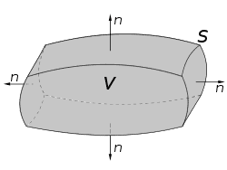
As it has been for the line integral of a vector field along a smooth curve, the surface integral (or the volume integral) of a vector field over a regular surface $S$ also depends on the orientation of the surface. To introduce the concept, let $\mathbf{r}=\mathbf{r}(u, v): \Omega \rightarrow$ $\mathbb{R}^3$ be a parametrisation of $S$. In general, we study the geometry of $S$ at a point $a=\left(u_0, v_0\right) \in \Omega$ by using the two (orthogonal) curves given by
$$
\mathbf{r}_1(u)=\mathbf{r}\left(u, v_0\right) \quad \text { and } \quad \mathbf{r}_2(v)=\mathbf{r}\left(u_0, v\right),
$$
respectively, called the $u$-curve and $v$-curve. Notice that the derivatives $\mathbf{r}_u=\mathbf{r}^{\prime}(u)$ and $\mathbf{r}_v=\mathbf{r}^{\prime}(v)$ are, respectively, the tangent vectors to the two curves $\mathbf{r}_1$ and $\mathbf{r}_2$ on $S$. Also, by the vector identity
$$
\left|\mathbf{r}_u \times \mathbf{r}_v\right|^2=\left(\mathbf{r}_u \times \mathbf{r}_v\right) \cdot\left(\mathbf{r}_u \times \mathbf{r}_v\right)=\operatorname{det}\left(\begin{array}{l}
\mathbf{r}_u \cdot \mathbf{r}_u \mathbf{r}_u \cdot \mathbf{r}_v \
\mathbf{r}_v \cdot \mathbf{r}_u \mathbf{r}_v \cdot \mathbf{r}_v
\end{array}\right)
$$
it follows that the regularity condition as given in Definition $2.27$ is equivalent to the condition that the vectors $\mathbf{r}_u, \mathbf{r}_v$ are linearly independent. Therefore, there is a unique (shifted) tangent plane $\Pi(a)$ at $\mathbf{r}(\boldsymbol{a}) \in S$ spanned by the tangent vectors $\mathbf{r}_u$ and $\mathbf{r}_v$. In fact, the two vectors form a natural basis for the tangent plane $\Pi(\boldsymbol{x})$ in the sense we explain shortly. In particular, if $\varphi \in C^1(\Omega)$, then for the regular surface $$
\Gamma_{\varphi}(x, y, z): \quad \varphi(x, y)-z=0,
$$
we have $\mathbf{r}x=\left(1,0, \varphi_x\right)$ and $\mathbf{r}_y=\left(0,1, \varphi_y\right)$, which implies that $$ \mathbf{r}_x \times \mathbf{r}_y=\left(-\varphi_x,-\varphi_y, 1\right), $$ and the equation of the tangent plane at a point $\boldsymbol{a}=\left(x_0, y_0, z_0\right)$ is given by $$ \varphi_x\left(x-x_0\right)+\varphi_y\left(y-y_0\right)-\left(z-z_0\right)=0, \quad \text { where } z_0=\varphi\left(x_0, y_0\right) . $$ Therefore, for any $x \in 1{\varphi}^{\prime}$, we have
$$
\mathbf{n}(\boldsymbol{x})=\pm \frac{\mathbf{r}_u \times \mathbf{r}_v}{\left|\mathbf{r}_u \times \mathbf{r}_v\right|}=\frac{\left(-\varphi_x,-\varphi_y, 1\right)}{\sqrt{\varphi_x^2+\varphi_y^2+1}}
$$
偏微分方程代写
数学代写|偏微分方程代写partial difference equations代考|Vector Calculus
矢量分析的发展主要归功于英国数学家 Oliver Heaviside (1850-1925),并独立于美国数学家Josiah
Gibbs (18391903)。Heaviside 于 1893 年发表了他的作品,作为“矢量代数和分析的要素”一书的一部分,
而吉布斯的作品首次出现是作为”矢量分析的要素”一书,于 1901 年出版,作为他在 1881 年发表的演讲的
汇编在耶鲁大学。Heaviside 应用矢量分析工具以矢量形式重新表述与电磁辐射相关的二十个方程中的十
二个,这些方程最初由苏格兰数学家和科学家 James Maxwell (1831-1879) 在 1861-62 年间提出。这十
二个方程在现代物理学中被公认为麦克斯韦四大基本方程(详见附录A.2)。
在本节中,我们将讨论高斯、斯托克斯和亥姆霍兹的三个基本定理,这些定理将在接下来的两章中应用, 以推导与流体流动、热传导、机械振动等物理现象相关的一些重要实际问题的微分方程模型, 和电磁波。
在接下来的所有内容中,前面介绍的 3 维 del 运算符起着主导作用。我们将使用如下所示的速记运算符符 믁:
$$
\partial_x \equiv \frac{\partial}{\partial x}, \quad \partial_y \equiv \frac{\partial}{\partial y}, \quad \partial_{x x} \equiv \frac{\partial^2}{\partial x^2}, \quad \partial_{y x} \equiv \frac{\partial^2}{\partial y \partial x}, \quad \text { etc. }
$$
让 $\Omega \subseteq \mathbb{R}^n$ 是一个域。回想一下 $C^1$-功能 $\varphi: \Omega \rightarrow \mathbb{R}_{\text {称为标量场,矢量场是 }} C^1$-功能 $f: \Omega \rightarrow \mathbb{R}^n$. 显 然,每个坐标函数 $f_i: \Omega \rightarrow \mathbb{R}$ 向量场 $f$ 是一个 $C^1$-标量场,对于 $i=1, \ldots, n$. 更一般地,对于 $k \geq 1$ , 向量场 $f$ 是一个 $C^k$-函数当且仅当每个坐标函数 $f_i \in C^k(\Omega)$. 也就是说,对于 $k \geq 1$ ,
$$
f=\left(f_1, \ldots, f_n\right) \in C^k(\Omega) \Leftrightarrow f_i \in C^k(\Omega), \text { for all } 1 \leq i \leq n .
$$
所以, $f$ 是一个 $C^{\infty}$-函数当且仅当每个坐标函数 $f_i \in C^{\infty}(\Omega)$. 在后一种情况下,我们还说 $f$ 是光滑矢量 场。类似的修改适用于适用于矢量场的其他符号和术语。我们主要处理的情况是 $n=2$ 或者 $n=3$.
定义 $2.29$ 对于 $I \subseteq \mathbb{R}$, 和一个域 $U \subseteq \mathbb{R}^n$ , 让 $\Omega=I \times U \subseteq \mathbb{R}^{n+1}$ , 和 $\boldsymbol{f}: U \rightarrow \mathbb{R}^n$ 是一个 $C^1$ 矢量 场。对于任何 $\left(t_0, \boldsymbol{x}_0\right) \in \Omega$ ,让 $\delta>0, \varepsilon>0$ 是这样的 $J=\left[t_0-\delta, t_0+\varepsilon\right] \subset I$.一个 $C^1$-功能 $\boldsymbol{x}:\left[t_0-\delta, t_0+\varepsilon\right] \rightarrow \Omega$ 称为场的积分曲线 $f$ 如果
$x^{\prime}(t)=f(x(t))$, for all $t \in J$, with $x\left(t_0\right)=x_0$.
数学代写|偏微分方程代写partial difference equations代考|Flux and Divergence Theorem
正如矢量场沿光滑曲线的线积分,矢量场在规则曲面上的表面积分(或体积积分) $S$ 还取决于表面的方 向。为了介绍这个概念,让 $\mathbf{r}=\mathbf{r}(u, v): \Omega \rightarrow \mathbb{R}^3$ 是一个参数化 $S$.一般来说,我们研究几何 $S$ 在某一点 $a=\left(u_0, v_0\right) \in \Omega$ 通过使用由给出的两条 (正交) 曲线
$$
\mathbf{r}1(u)=\mathbf{r}\left(u, v_0\right) \quad \text { and } \quad \mathbf{r}_2(v)=\mathbf{r}\left(u_0, v\right), $$ 分别称为 $u$-曲线和 $v$-曲线。注意导数 $\mathbf{r}_u=\mathbf{r}^{\prime}(u)$ 和 $\mathbf{r}_v=\mathbf{r}^{\prime}(v)$ 分别是两条曲线的切向量 $\mathbf{r}_1$ 和 $\mathbf{r}_2$ 上 $S$. 此 外,通过矢量标识 $$ \left|\mathbf{r}_u \times \mathbf{r}_v\right|^2=\left(\mathbf{r}_u \times \mathbf{r}_v\right) \cdot\left(\mathbf{r}_u \times \mathbf{r}_v\right)=\operatorname{det}\left(\mathbf{r}_u \cdot \mathbf{r}_u \mathbf{r}_u \cdot \mathbf{r}_v \mathbf{r}_v \cdot \mathbf{r}_u \mathbf{r}_v \cdot \mathbf{r}_v\right) $$ 由此得出定义中给出的规律性条件 $2.27$ 等同于向量的条件 $\mathbf{r}_u, \mathbf{r}_v$ 是线性独立的。因此,存在唯一的(移动 的)切平面 $\Pi(a)$ 在 $\mathbf{r}(\boldsymbol{a}) \in S$ 由切向量跨越 $\mathbf{r}_u$ 和 $\mathbf{r}_v$. 事实上,这两个向量构成了切平面的自然基础 $\Pi(\boldsymbol{x})$ 从某种意义上说,我们很快就会解释。特别是,如果 $\varphi \in C^1(\Omega)$ ,那么对于规则曲面 $$ \Gamma{\varphi}(x, y, z): \quad \varphi(x, y)-z=0,
$$
我们有 $\mathbf{r} x=\left(1,0, \varphi_x\right)$ 和 $\mathbf{r}_y=\left(0,1, \varphi_y\right)$ ,这意味着
$$
\mathbf{r}_x \times \mathbf{r}_y=\left(-\varphi_x,-\varphi_y, 1\right),
$$
和切平面在一点的方程 $\boldsymbol{a}=\left(x_0, y_0, z_0\right)$ 是(谁) 给的
$$
\varphi_x\left(x-x_0\right)+\varphi_y\left(y-y_0\right)-\left(z-z_0\right)=0, \quad \text { where } z_0=\varphi\left(x_0, y_0\right) .
$$
因此,对于任何 $x \in 1 \varphi^{\prime}$ , 我们有
$$
\mathbf{n}(\boldsymbol{x})=\pm \frac{\mathbf{r}_u \times \mathbf{r}_v}{\left|\mathbf{r}_u \times \mathbf{r}_v\right|}=\frac{\left(-\varphi_x,-\varphi_y, 1\right)}{\sqrt{\varphi_x^2+\varphi_y^2+1}}
$$

统计代写请认准statistics-lab™. statistics-lab™为您的留学生涯保驾护航。
金融工程代写
金融工程是使用数学技术来解决金融问题。金融工程使用计算机科学、统计学、经济学和应用数学领域的工具和知识来解决当前的金融问题,以及设计新的和创新的金融产品。
非参数统计代写
非参数统计指的是一种统计方法,其中不假设数据来自于由少数参数决定的规定模型;这种模型的例子包括正态分布模型和线性回归模型。
广义线性模型代考
广义线性模型(GLM)归属统计学领域,是一种应用灵活的线性回归模型。该模型允许因变量的偏差分布有除了正态分布之外的其它分布。
术语 广义线性模型(GLM)通常是指给定连续和/或分类预测因素的连续响应变量的常规线性回归模型。它包括多元线性回归,以及方差分析和方差分析(仅含固定效应)。
有限元方法代写
有限元方法(FEM)是一种流行的方法,用于数值解决工程和数学建模中出现的微分方程。典型的问题领域包括结构分析、传热、流体流动、质量运输和电磁势等传统领域。
有限元是一种通用的数值方法,用于解决两个或三个空间变量的偏微分方程(即一些边界值问题)。为了解决一个问题,有限元将一个大系统细分为更小、更简单的部分,称为有限元。这是通过在空间维度上的特定空间离散化来实现的,它是通过构建对象的网格来实现的:用于求解的数值域,它有有限数量的点。边界值问题的有限元方法表述最终导致一个代数方程组。该方法在域上对未知函数进行逼近。[1] 然后将模拟这些有限元的简单方程组合成一个更大的方程系统,以模拟整个问题。然后,有限元通过变化微积分使相关的误差函数最小化来逼近一个解决方案。
tatistics-lab作为专业的留学生服务机构,多年来已为美国、英国、加拿大、澳洲等留学热门地的学生提供专业的学术服务,包括但不限于Essay代写,Assignment代写,Dissertation代写,Report代写,小组作业代写,Proposal代写,Paper代写,Presentation代写,计算机作业代写,论文修改和润色,网课代做,exam代考等等。写作范围涵盖高中,本科,研究生等海外留学全阶段,辐射金融,经济学,会计学,审计学,管理学等全球99%专业科目。写作团队既有专业英语母语作者,也有海外名校硕博留学生,每位写作老师都拥有过硬的语言能力,专业的学科背景和学术写作经验。我们承诺100%原创,100%专业,100%准时,100%满意。
随机分析代写
随机微积分是数学的一个分支,对随机过程进行操作。它允许为随机过程的积分定义一个关于随机过程的一致的积分理论。这个领域是由日本数学家伊藤清在第二次世界大战期间创建并开始的。
时间序列分析代写
随机过程,是依赖于参数的一组随机变量的全体,参数通常是时间。 随机变量是随机现象的数量表现,其时间序列是一组按照时间发生先后顺序进行排列的数据点序列。通常一组时间序列的时间间隔为一恒定值(如1秒,5分钟,12小时,7天,1年),因此时间序列可以作为离散时间数据进行分析处理。研究时间序列数据的意义在于现实中,往往需要研究某个事物其随时间发展变化的规律。这就需要通过研究该事物过去发展的历史记录,以得到其自身发展的规律。
回归分析代写
多元回归分析渐进(Multiple Regression Analysis Asymptotics)属于计量经济学领域,主要是一种数学上的统计分析方法,可以分析复杂情况下各影响因素的数学关系,在自然科学、社会和经济学等多个领域内应用广泛。
MATLAB代写
MATLAB 是一种用于技术计算的高性能语言。它将计算、可视化和编程集成在一个易于使用的环境中,其中问题和解决方案以熟悉的数学符号表示。典型用途包括:数学和计算算法开发建模、仿真和原型制作数据分析、探索和可视化科学和工程图形应用程序开发,包括图形用户界面构建MATLAB 是一个交互式系统,其基本数据元素是一个不需要维度的数组。这使您可以解决许多技术计算问题,尤其是那些具有矩阵和向量公式的问题,而只需用 C 或 Fortran 等标量非交互式语言编写程序所需的时间的一小部分。MATLAB 名称代表矩阵实验室。MATLAB 最初的编写目的是提供对由 LINPACK 和 EISPACK 项目开发的矩阵软件的轻松访问,这两个项目共同代表了矩阵计算软件的最新技术。MATLAB 经过多年的发展,得到了许多用户的投入。在大学环境中,它是数学、工程和科学入门和高级课程的标准教学工具。在工业领域,MATLAB 是高效研究、开发和分析的首选工具。MATLAB 具有一系列称为工具箱的特定于应用程序的解决方案。对于大多数 MATLAB 用户来说非常重要,工具箱允许您学习和应用专业技术。工具箱是 MATLAB 函数(M 文件)的综合集合,可扩展 MATLAB 环境以解决特定类别的问题。可用工具箱的领域包括信号处理、控制系统、神经网络、模糊逻辑、小波、仿真等。