标签: MPH 701

统计代写|生物统计代写Biostatistics代考|MPH203

如果你也在 怎样代写生物统计Biostatistics这个学科遇到相关的难题,请随时右上角联系我们的24/7代写客服。

生物统计学是将统计技术应用于健康相关领域的科学研究,包括医学、生物学和公共卫生,并开发新的工具来研究这些领域。

statistics-lab™ 为您的留学生涯保驾护航 在代写生物统计Biostatistics方面已经树立了自己的口碑, 保证靠谱, 高质且原创的统计Statistics代写服务。我们的专家在代写生物统计Biostatistics代写方面经验极为丰富,各种生物统计Biostatistics相关的作业也就用不着说。

我们提供的生物统计Biostatistics及其相关学科的代写,服务范围广, 其中包括但不限于:

  • Statistical Inference 统计推断
  • Statistical Computing 统计计算
  • Advanced Probability Theory 高等概率论
  • Advanced Mathematical Statistics 高等数理统计学
  • (Generalized) Linear Models 广义线性模型
  • Statistical Machine Learning 统计机器学习
  • Longitudinal Data Analysis 纵向数据分析
  • Foundations of Data Science 数据科学基础
统计代写|生物统计代写Biostatistics代考|MPH203

统计代写|生物统计代写Biostatistics代考|Proportions and Percentiles

Populations are often summarized by listing the important percentages or proportions associated with the population. The proportion of units in a population having a particular characteristic is a parameter of the population, and a population proportion will be denoted by $p$. The population proportion having a particular characteristic, say characteristic $\mathrm{A}$, is defined to be
$$
p=\frac{\text { number of units in population having characteristic A }}{N}
$$
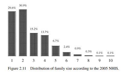
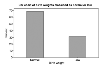
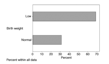
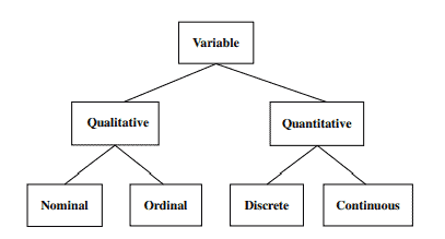
Note that the percentage of the population having characteristic A is $p \times 100 \%$. Population proportions and percentages are often associated with the categories of a qualitative variable or with the values in the population falling in a specific range of values. For example, the distribution of a qualitative variable is usually displayed in a bar chart with the height of a bar representing either the proportion or percentage of the population having that particular value.
Example $2.12$
The distribution of blood type according to the American Red Cross is given in Table $2.4$ in terms of proportions.

An important proportion in many biomedical studies is the proportion of individuals having a particular disease, which is called the prevalence of the disease. The prevalence of a disease is defined to be
Prevalence $=$ The proportion of individuals in a well-defined population having the disease of interest
For example, according to the Centers for Disease Control and Prevention (CDC) the prevalence of smoking among adults in the United States in January through June 2005 was $20.9 \%$. Proportions also play important roles in the study of survival and cure rates, the occurrence of side effects of new drugs, the absolute and relative risks associated with a disease, and the efficacy of new treatments and drugs.

A parameter that is related to a population proportion for a quantitative variable is the pth percentile of the population. The pth percentile is the value in the population where $p$ percent of the population falls below this value. The pth percentile will be denoted by $x_p$ for values of $p$ between 0 and 100 .

统计代写|生物统计代写Biostatistics代考|Parameters Measuring

The two parameters in the population of values of a quantitative variable that summarize how the variable is distributed are the parameters that measure the typical or central values in the population and the parameters that measure the spread of the values within the population. Parameters describing the central values in a population and the spread of a population are often used for summarizing the distribution of the values in a population; however, it is important to note that most populations cannot be described very well with only the parameters that measure centrality and the spread of the population.

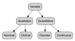
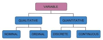
Measures of centrality, location, or the typical value are parameters that lie in the “center” or “middle” region of a distribution. Because the center or middle of a distribution is not easily determined due to the wide range of different shapes that are possible with a distribution, there are several different parameters that can be used to describe the center of a population. The three most commonly used parameters for describing the center of a population are the mean, median, and mode. For a quantitative variable $X$.

  • The mean of a population is the average of all of the units in the population, and will be denoted by $\mu$. The mean of a variable $X$ measured on a population consisting of $N$ units is
    $$
    \mu=\frac{\text { sum of the values of } X}{N}=\frac{\sum X}{N}
    $$
  • The median of a population is the 50 th percentile of the population, and will be denoted by $\tilde{\mu}$. The median of a population is found by first listing all of the values of the variable $X$, including repeated $X$ values, in ascending order. When the number of units in the population (i.e., $N$ ) is an odd number, the median is the middle observation in the list of ordered values of $X$; when $N$ is an even number, the median will be the average of the two observations in the middle of the ordered list of $X$ values.
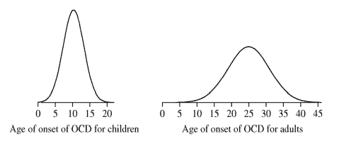
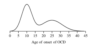
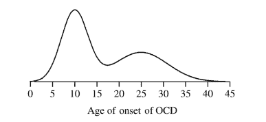
  • The mode of a population is the most frequent value in the population, and will be denoted by $M$. In a graph of the probability density function, the mode is the value of $X$ under the peak of the graph, and a population can have more than one mode as shown in Figure 2.8.

The mean, median, and mode are three different parameters that can be used to measure the center of a population or to describe the typical values in a population. These three parameters will have nearly the same value when the distribution is symmetric or mound shaped. For long-tailed distributions, the mean, median, and mode will be different, and the difference in their values will depend on the length of the distribution’s longer tail. Figures $2.12$ and $2.13$ illustrate the relationships between the values of the mean, median, and mode for long-tail right and long-tail left distributions.

统计代写|生物统计代写Biostatistics代考|MPH203

生物统计代考

统计代写|生物统计代写Biostatistics代考|Proportions and Percentiles

人口通常通过列出与人口相关的重要百分比或比例来总结。人口中具有特定特征的单位的比例是人口的一个参数,人口比例将表示为p. 具有特定特征的人口比例,比如特征一个, 定义为

p= 人口中具有特征 A 的单位数 ñ
请注意,具有特征 A 的总体百分比是p×100%. 人口比例和百分比通常与定性变量的类别或与落在特定值范围内的人口值相关联。例如,定性变量的分布通常显示在条形图中,条形的高度代表具有该特定值的总体的比例或百分比。
例子2.12
美国红十字会血型分布见表2.4从比例上看。

在许多生物医学研究中,一个重要的比例是个体患有特定疾病的比例,这被称为疾病的患病率。疾病的患病率定义为
患病率=明确定义的人群中患有相关疾病的个体比例
例如,根据疾病控制和预防中心 (CDC) 的数据,2005 年 1 月至 2005 年 6 月美国成年人的吸烟率是20.9%. 比例在研究生存率和治愈率、新药副作用的发生、与疾病相关的绝对和相对风险以及新疗法和药物的疗效等方面也发挥着重要作用。

与定量变量的总体比例相关的参数是总体的第 p 个百分位数。第 p 个百分位数是总体中的值,其中p人口的百分比低于这个值。第 p 个百分位数将表示为Xp对于值p0 到 100 之间。

统计代写|生物统计代写Biostatistics代考|Parameters Measuring

量化变量值总体中总结变量分布方式的两个参数是测量总体中的典型值或中心值的参数,以及测量值在总体中分布的参数。描述总体中的中心值和总体分布的参数通常用于总结总体中值的分布;然而,重要的是要注意,仅使用衡量中心性和人口分布的参数无法很好地描述大多数人口。

中心性、位置或典型值的度量是位于分布“中心”或“中间”区域的参数。由于分布可能具有多种不同形状,因此不容易确定分布的中心或中间,因此可以使用几个不同的参数来描述总体的中心。用于描述总体中心的三个最常用的参数是均值、中位数和众数。对于定量变量X.

  • 总体的平均值是总体中所有单位的平均值,表示为米. 变量的平均值X在由以下人员组成的总体上测量ñ单位是
    米= 的值的总和 Xñ=∑Xñ
  • 人口的中位数是人口的第 50 个百分位,表示为米~. 通过首先列出变量的所有值来找到总体的中位数X,包括重复X值,按升序排列。当人口中的单位数(即,ñ) 是奇数,中位数是 的有序值列表中的中间观察值X; 什么时候ñ是偶数,中位数将是有序列表中间的两个观察值的平均值X价值观。
  • 人口的众数是人口中出现频率最高的值,记为米. 在概率密度函数图中,众数是X如图 2.8 所示,一个总体可以有多个众数。

均值、中位数和众数是三个不同的参数,可用于衡量总体中心或描述总体中的典型值。当分布是对称或丘状时,这三个参数将具有几乎相同的值。对于长尾分布,均值、中位数和众数会有所不同,它们值的差异将取决于分布较长尾的长度。数字2.12和2.13说明长尾右分布和长尾左分布的均值、中值和众数之间的关系。

统计代写|生物统计代写Biostatistics代考 请认准statistics-lab™

统计代写请认准statistics-lab™. statistics-lab™为您的留学生涯保驾护航。

金融工程代写

金融工程是使用数学技术来解决金融问题。金融工程使用计算机科学、统计学、经济学和应用数学领域的工具和知识来解决当前的金融问题,以及设计新的和创新的金融产品。

非参数统计代写

非参数统计指的是一种统计方法,其中不假设数据来自于由少数参数决定的规定模型;这种模型的例子包括正态分布模型和线性回归模型。

广义线性模型代考

广义线性模型(GLM)归属统计学领域,是一种应用灵活的线性回归模型。该模型允许因变量的偏差分布有除了正态分布之外的其它分布。

术语 广义线性模型(GLM)通常是指给定连续和/或分类预测因素的连续响应变量的常规线性回归模型。它包括多元线性回归,以及方差分析和方差分析(仅含固定效应)。

有限元方法代写

有限元方法(FEM)是一种流行的方法,用于数值解决工程和数学建模中出现的微分方程。典型的问题领域包括结构分析、传热、流体流动、质量运输和电磁势等传统领域。

有限元是一种通用的数值方法,用于解决两个或三个空间变量的偏微分方程(即一些边界值问题)。为了解决一个问题,有限元将一个大系统细分为更小、更简单的部分,称为有限元。这是通过在空间维度上的特定空间离散化来实现的,它是通过构建对象的网格来实现的:用于求解的数值域,它有有限数量的点。边界值问题的有限元方法表述最终导致一个代数方程组。该方法在域上对未知函数进行逼近。[1] 然后将模拟这些有限元的简单方程组合成一个更大的方程系统,以模拟整个问题。然后,有限元通过变化微积分使相关的误差函数最小化来逼近一个解决方案。

tatistics-lab作为专业的留学生服务机构,多年来已为美国、英国、加拿大、澳洲等留学热门地的学生提供专业的学术服务,包括但不限于Essay代写,Assignment代写,Dissertation代写,Report代写,小组作业代写,Proposal代写,Paper代写,Presentation代写,计算机作业代写,论文修改和润色,网课代做,exam代考等等。写作范围涵盖高中,本科,研究生等海外留学全阶段,辐射金融,经济学,会计学,审计学,管理学等全球99%专业科目。写作团队既有专业英语母语作者,也有海外名校硕博留学生,每位写作老师都拥有过硬的语言能力,专业的学科背景和学术写作经验。我们承诺100%原创,100%专业,100%准时,100%满意。

随机分析代写


随机微积分是数学的一个分支,对随机过程进行操作。它允许为随机过程的积分定义一个关于随机过程的一致的积分理论。这个领域是由日本数学家伊藤清在第二次世界大战期间创建并开始的。

时间序列分析代写

随机过程,是依赖于参数的一组随机变量的全体,参数通常是时间。 随机变量是随机现象的数量表现,其时间序列是一组按照时间发生先后顺序进行排列的数据点序列。通常一组时间序列的时间间隔为一恒定值(如1秒,5分钟,12小时,7天,1年),因此时间序列可以作为离散时间数据进行分析处理。研究时间序列数据的意义在于现实中,往往需要研究某个事物其随时间发展变化的规律。这就需要通过研究该事物过去发展的历史记录,以得到其自身发展的规律。

回归分析代写

多元回归分析渐进(Multiple Regression Analysis Asymptotics)属于计量经济学领域,主要是一种数学上的统计分析方法,可以分析复杂情况下各影响因素的数学关系,在自然科学、社会和经济学等多个领域内应用广泛。

MATLAB代写

MATLAB 是一种用于技术计算的高性能语言。它将计算、可视化和编程集成在一个易于使用的环境中,其中问题和解决方案以熟悉的数学符号表示。典型用途包括:数学和计算算法开发建模、仿真和原型制作数据分析、探索和可视化科学和工程图形应用程序开发,包括图形用户界面构建MATLAB 是一个交互式系统,其基本数据元素是一个不需要维度的数组。这使您可以解决许多技术计算问题,尤其是那些具有矩阵和向量公式的问题,而只需用 C 或 Fortran 等标量非交互式语言编写程序所需的时间的一小部分。MATLAB 名称代表矩阵实验室。MATLAB 最初的编写目的是提供对由 LINPACK 和 EISPACK 项目开发的矩阵软件的轻松访问,这两个项目共同代表了矩阵计算软件的最新技术。MATLAB 经过多年的发展,得到了许多用户的投入。在大学环境中,它是数学、工程和科学入门和高级课程的标准教学工具。在工业领域,MATLAB 是高效研究、开发和分析的首选工具。MATLAB 具有一系列称为工具箱的特定于应用程序的解决方案。对于大多数 MATLAB 用户来说非常重要,工具箱允许您学习应用专业技术。工具箱是 MATLAB 函数(M 文件)的综合集合,可扩展 MATLAB 环境以解决特定类别的问题。可用工具箱的领域包括信号处理、控制系统、神经网络、模糊逻辑、小波、仿真等。

R语言代写问卷设计与分析代写
PYTHON代写回归分析与线性模型代写
MATLAB代写方差分析与试验设计代写
STATA代写机器学习/统计学习代写
SPSS代写计量经济学代写
EVIEWS代写时间序列分析代写
EXCEL代写深度学习代写
SQL代写各种数据建模与可视化代写

统计代写|生物统计代写Biostatistics代考|MPH701

如果你也在 怎样代写生物统计Biostatistics这个学科遇到相关的难题,请随时右上角联系我们的24/7代写客服。

生物统计学是将统计技术应用于健康相关领域的科学研究,包括医学、生物学和公共卫生,并开发新的工具来研究这些领域。

statistics-lab™ 为您的留学生涯保驾护航 在代写生物统计Biostatistics方面已经树立了自己的口碑, 保证靠谱, 高质且原创的统计Statistics代写服务。我们的专家在代写生物统计Biostatistics代写方面经验极为丰富,各种生物统计Biostatistics相关的作业也就用不着说。

我们提供的生物统计Biostatistics及其相关学科的代写,服务范围广, 其中包括但不限于:

  • Statistical Inference 统计推断
  • Statistical Computing 统计计算
  • Advanced Probability Theory 高等概率论
  • Advanced Mathematical Statistics 高等数理统计学
  • (Generalized) Linear Models 广义线性模型
  • Statistical Machine Learning 统计机器学习
  • Longitudinal Data Analysis 纵向数据分析
  • Foundations of Data Science 数据科学基础
统计代写|生物统计代写Biostatistics代考|MPH701

统计代写|生物统计代写Biostatistics代考|Quantitative Variables

A quantitative variable is a variable that takes only numeric values. The values of a quantitative variable are said to be measured on an interval scale when the difference between two values is meaningful; the values of a quantitative variable are said to be measured on a ratio scale when the ratio of two values is meaningful. The key difference between a variable measured on an interval scale and a ratio scale is that on a ratio scale there is a “natural zero” representing absence of the attribute being measured, while there is no natural zero for variables measured on only an interval scale. Some scales of measurement will have natural zero and some will not. When a measurement scale has a natural zero, then the ratio of two measurements is a meaningful measure of how many times larger one value is than the other. For example, the variable Fat that represents the grams of fat in a food product is measured on a ratio scale because the value Fat $=0$ indicates that the unit contained absolutely no fat. When a scale of measurement does not have a natural zero, then only the difference between two measurements is a meaningful comparison of the values of the two measurements. For example, the variable Body Temperature is measured on a scale that has no natural zero since Body Temperature $=0$ does not indicate that the body has no temperature.

Since interval scales are ordered, the difference between two values measures how much larger one value is than another. A ratio scale is also an interval scale but has the additional property that the ratio of two values is meaningful. Thus, for a variable measured on an interval scale the difference of two values is the meaningful way to compare the values, and for a variable measured on a ratio scale both the difference and the ratio of two values are meaningful ways to compare difference values of the variable. For example, body temperature in degrees Fahrenheit is a variable that is measured on an interval scale so that it is meaningful to say that a body temperature of $98.6$ and a body temperature of $102.3$ differ by $3.7$ degrees; however, it would not be meaningful to say that a temperature of $102.3$ is $1.04$ times as much as a temperature of $98.6$. On the other hand, the variable weight in pounds is measured on a ratio scale, and therefore, it would be proper to say that a weight of $210 \mathrm{lb}$ is $1.4$ times a weight of $150 \mathrm{lb}$; it would also be meaningful to say that a weight of $210 \mathrm{lb}$ is $60 \mathrm{lb}$ more than a weight of $150 \mathrm{lb}$.

统计代写|生物统计代写Biostatistics代考|POPULATION DISTRIBUTIONS AND PARAMETERS

For a well-defined population of units and a variable, say $X$, the collection of all possible values of the variable $X$ formed by measuring all of the units in the target population forms the population associated with the variable $X$. When multiple variables are recorded, each of the variables will generate its own population. Furthermore, since a variable may take on many different values, an important question concerning the population of values of the variable is “How can the population of values of a variable be described or summarized?” The two different approaches that can be used to describe the population of values of the variable are (1) to describe explicitly how the variable is distributed over its values and (2) to describe a set of characteristics that summarize the distribution of the values in the population.

A statistical analysis of a population is centered on how the values of a variable are distributed, and the distribution of a variable or population is an explicit description of how the values of the variable are distributed often described in terms of percentages. The distribution of a variable is also called a probability distribution because it describes the probabilities that each of the possible values of the variable will occur. Moreover, the distribution of a variable is often presented in table or chart or modeled with a mathematical equation that explicitly determines the percentage of the population taking on each possible value of the variable. The total percentage in a probability distribution is $100 \%$. The distribution of a qualitative or a discrete variable is generally displayed in a bar chart or in a table, and the distribution of a continuous variable is generally displayed in a graph or is represented by a mathematical function.

统计代写|生物统计代写Biostatistics代考|MPH701

生物统计代考

统计代写|生物统计代写Biostatistics代考|Quantitative Variables

定量变量是只取数值的变量。当两个值之间的差异有意义时,就说定量变量的值是在区间尺度上测量的;当两个值的比率有意义时,就可以说定量变量的值是在比率尺度上测量的。在区间尺度和比率尺度上测量的变量之间的主要区别在于,在比率尺度上,有一个“自然零”表示不存在被测量的属性,而仅在区间尺度上测量的变量没有自然零. 一些测量尺度将具有自然零,而一些则没有。当测量尺度具有自然零时,两个测量值的比率是一个有意义的度量,用于衡量一个值比另一个值大多少倍。例如,=0表示该单位绝对不含脂肪。当测量尺度没有自然零时,只有两次测量之间的差异才是两次测量值的有意义的比较。例如,变量体温是在一个没有自然零的标度上测量的,因为体温=0并不表示身体没有温度。

由于区间尺度是有序的,因此两个值之间的差值衡量一个值比另一个值大多少。比率刻度也是一个区间刻度,但具有两个值的比率有意义的附加属性。因此,对于在区间尺度上测量的变量,两个值的差异是比较值的有意义的方式,而对于在比率尺度上测量的变量,两个值的差异和比率都是比较差异值的有意义的方式变量。例如,以华氏度为单位的体温是一个在区间尺度上测量的变量,因此说体温为98.6和体温102.3区别于3.7学位;然而,说温度为102.3是1.04温度的几倍98.6. 另一方面,以磅为单位的可变重量是在比例尺度上测量的,因此,可以说重量为210lb是1.4重量的倍150lb; 说一个重量210lb是60lb超过一个重量150lb.

统计代写|生物统计代写Biostatistics代考|POPULATION DISTRIBUTIONS AND PARAMETERS

对于定义明确的单位群体和变量,例如X, 变量所有可能值的集合X通过测量目标人口中的所有单位形成的人口与变量相关联X. 当记录多个变量时,每个变量都会产生自己的总体。此外,由于一个变量可能具有许多不同的值,因此有关变量值总体的一个重要问题是“如何描述或总结变量的值总体?” 可用于描述变量值总体的两种不同方法是:(1)明确描述变量如何在其值上分布;(2)描述一组特征,总结了变量中值的分布。人口。

总体的统计分析以变量的值如何分布为中心,而变量或总体的分布是对变量值如何分布的明确描述,通常以百分比来描述。变量的分布也称为概率分布,因为它描述了变量的每个可能值出现的概率。此外,变量的分布通常以表格或图表的形式呈现,或者用一个数学方程建模,该方程明确地确定了接受变量每个可能值的总体百分比。概率分布中的总百分比是100%. 定性或离散变量的分布一般以条形图或表格的形式显示,连续变量的分布一般以图形或数学函数的形式表示。

统计代写|生物统计代写Biostatistics代考 请认准statistics-lab™

统计代写请认准statistics-lab™. statistics-lab™为您的留学生涯保驾护航。

金融工程代写

金融工程是使用数学技术来解决金融问题。金融工程使用计算机科学、统计学、经济学和应用数学领域的工具和知识来解决当前的金融问题,以及设计新的和创新的金融产品。

非参数统计代写

非参数统计指的是一种统计方法,其中不假设数据来自于由少数参数决定的规定模型;这种模型的例子包括正态分布模型和线性回归模型。

广义线性模型代考

广义线性模型(GLM)归属统计学领域,是一种应用灵活的线性回归模型。该模型允许因变量的偏差分布有除了正态分布之外的其它分布。

术语 广义线性模型(GLM)通常是指给定连续和/或分类预测因素的连续响应变量的常规线性回归模型。它包括多元线性回归,以及方差分析和方差分析(仅含固定效应)。

有限元方法代写

有限元方法(FEM)是一种流行的方法,用于数值解决工程和数学建模中出现的微分方程。典型的问题领域包括结构分析、传热、流体流动、质量运输和电磁势等传统领域。

有限元是一种通用的数值方法,用于解决两个或三个空间变量的偏微分方程(即一些边界值问题)。为了解决一个问题,有限元将一个大系统细分为更小、更简单的部分,称为有限元。这是通过在空间维度上的特定空间离散化来实现的,它是通过构建对象的网格来实现的:用于求解的数值域,它有有限数量的点。边界值问题的有限元方法表述最终导致一个代数方程组。该方法在域上对未知函数进行逼近。[1] 然后将模拟这些有限元的简单方程组合成一个更大的方程系统,以模拟整个问题。然后,有限元通过变化微积分使相关的误差函数最小化来逼近一个解决方案。

tatistics-lab作为专业的留学生服务机构,多年来已为美国、英国、加拿大、澳洲等留学热门地的学生提供专业的学术服务,包括但不限于Essay代写,Assignment代写,Dissertation代写,Report代写,小组作业代写,Proposal代写,Paper代写,Presentation代写,计算机作业代写,论文修改和润色,网课代做,exam代考等等。写作范围涵盖高中,本科,研究生等海外留学全阶段,辐射金融,经济学,会计学,审计学,管理学等全球99%专业科目。写作团队既有专业英语母语作者,也有海外名校硕博留学生,每位写作老师都拥有过硬的语言能力,专业的学科背景和学术写作经验。我们承诺100%原创,100%专业,100%准时,100%满意。

随机分析代写


随机微积分是数学的一个分支,对随机过程进行操作。它允许为随机过程的积分定义一个关于随机过程的一致的积分理论。这个领域是由日本数学家伊藤清在第二次世界大战期间创建并开始的。

时间序列分析代写

随机过程,是依赖于参数的一组随机变量的全体,参数通常是时间。 随机变量是随机现象的数量表现,其时间序列是一组按照时间发生先后顺序进行排列的数据点序列。通常一组时间序列的时间间隔为一恒定值(如1秒,5分钟,12小时,7天,1年),因此时间序列可以作为离散时间数据进行分析处理。研究时间序列数据的意义在于现实中,往往需要研究某个事物其随时间发展变化的规律。这就需要通过研究该事物过去发展的历史记录,以得到其自身发展的规律。

回归分析代写

多元回归分析渐进(Multiple Regression Analysis Asymptotics)属于计量经济学领域,主要是一种数学上的统计分析方法,可以分析复杂情况下各影响因素的数学关系,在自然科学、社会和经济学等多个领域内应用广泛。

MATLAB代写

MATLAB 是一种用于技术计算的高性能语言。它将计算、可视化和编程集成在一个易于使用的环境中,其中问题和解决方案以熟悉的数学符号表示。典型用途包括:数学和计算算法开发建模、仿真和原型制作数据分析、探索和可视化科学和工程图形应用程序开发,包括图形用户界面构建MATLAB 是一个交互式系统,其基本数据元素是一个不需要维度的数组。这使您可以解决许多技术计算问题,尤其是那些具有矩阵和向量公式的问题,而只需用 C 或 Fortran 等标量非交互式语言编写程序所需的时间的一小部分。MATLAB 名称代表矩阵实验室。MATLAB 最初的编写目的是提供对由 LINPACK 和 EISPACK 项目开发的矩阵软件的轻松访问,这两个项目共同代表了矩阵计算软件的最新技术。MATLAB 经过多年的发展,得到了许多用户的投入。在大学环境中,它是数学、工程和科学入门和高级课程的标准教学工具。在工业领域,MATLAB 是高效研究、开发和分析的首选工具。MATLAB 具有一系列称为工具箱的特定于应用程序的解决方案。对于大多数 MATLAB 用户来说非常重要,工具箱允许您学习应用专业技术。工具箱是 MATLAB 函数(M 文件)的综合集合,可扩展 MATLAB 环境以解决特定类别的问题。可用工具箱的领域包括信号处理、控制系统、神经网络、模糊逻辑、小波、仿真等。

R语言代写问卷设计与分析代写
PYTHON代写回归分析与线性模型代写
MATLAB代写方差分析与试验设计代写
STATA代写机器学习/统计学习代写
SPSS代写计量经济学代写
EVIEWS代写时间序列分析代写
EXCEL代写深度学习代写
SQL代写各种数据建模与可视化代写

统计代写|生物统计代写Biostatistics代考|STA310

如果你也在 怎样代写生物统计Biostatistics这个学科遇到相关的难题,请随时右上角联系我们的24/7代写客服。

生物统计学是将统计技术应用于健康相关领域的科学研究,包括医学、生物学和公共卫生,并开发新的工具来研究这些领域。

statistics-lab™ 为您的留学生涯保驾护航 在代写生物统计Biostatistics方面已经树立了自己的口碑, 保证靠谱, 高质且原创的统计Statistics代写服务。我们的专家在代写生物统计Biostatistics代写方面经验极为丰富,各种生物统计Biostatistics相关的作业也就用不着说。

我们提供的生物统计Biostatistics及其相关学科的代写,服务范围广, 其中包括但不限于:

  • Statistical Inference 统计推断
  • Statistical Computing 统计计算
  • Advanced Probability Theory 高等概率论
  • Advanced Mathematical Statistics 高等数理统计学
  • (Generalized) Linear Models 广义线性模型
  • Statistical Machine Learning 统计机器学习
  • Longitudinal Data Analysis 纵向数据分析
  • Foundations of Data Science 数据科学基础
统计代写|生物统计代写Biostatistics代考|STA310

统计代写|生物统计代写Biostatistics代考|POPULATIONS AND VARIABLES

In a properly designed biomedical research study, a well-defined target population and a particular set of research questions dictate the variables that should be measured on the units being studied in the research project. In most research problems, there are many variables that must be measured on each unit in the population. The outcome variables that are of primary interest are called the response variables, and the variables that are believed to explain the response variables are called the explanatory variables or predictor variables. For example, in a clinical trial designed to study the efficacy of a specialized treatment designed to reduce the size of a malignant tumor, the following explanatory variables might be recorded for each patient in the study: age, gender, race, weight, height, blood type, blood pressure, and oxygen uptake. The response variable in this study might be change in the size of the tumor.

Variables come in a variety of different types; however, each variable can be classified as being either quantitative or qualitative in nature. A variable that takes on only numeric values is a quantitative variable, and a variable that takes on non-numeric values is called a qualitative variable or a categorical variable. Note that a variable is a quantitative or qualitative variable based on the possible values the variable can take on.
Example $2.1$
In a study of obesity in the population of children aged 10 or less in the United States, some possible quantitative variables that might be measured include age, height, weight, heart rate, body mass index, and percent body fat; some qualitative variables that might be measured on this population include gender, eye color, race, and blood type. A likely choice for the response variable in this study would be the qualitative variable Obese defined by
$$
\text { Obese }= \begin{cases}\text { Yes } & \text { for a body mass index of }>30 \ \text { No } & \text { for a body mass index of } \leq 30\end{cases}
$$

统计代写|生物统计代写Biostatistics代考|Qualitative Variables

Qualitative variables take on nonnumeric values and are usually used to represent a distinct quality of a population unit. When the possible values of a qualitative variable have no intrinsic ordering, the variable is called a nominal variable; when there is a natural ordering of the possible values of the variable, then the variable is called an ordinal variable. An example of a nominal variable is Blood Type where the standard values for blood type are $\mathrm{A}, \mathrm{B}, \mathrm{AB}$, and $\mathrm{O}$. Clearly, there is no intrinsic ordering of these blood types, and hence, Blood Type is a nominal variable. An example of an ordinal variable is the variable Pain where a subject is asked to describe their pain verbally as

  • No pain,
  • Mild pain,
  • Discomforting pain,
  • Distressing pain,
  • Intense pain,
  • Excruciating pain.
    In this case, since the verbal descriptions describe increasing levels of pain, there is a clear ordering of the possible values of the variable Pain levels, and therefore, Pain is an ordinal qualitative variable.
    Example 2.2
    In the Framingham Heart Study of coronary heart disease, the following two nominal qualitative variables were recorded:
    $$
    \text { Smokes }=\left{\begin{array}{l}
    \text { Yes } \
    \text { No }
    \end{array}\right.
    $$ and
  • $$
  • \text { Diabetes }=\left{\begin{array}{l}
  • \text { Yes } \
  • \text { No }
  • \end{array}\right.
  • $$
  • Example $2.3$
  • An example of an ordinal variable is the variable Baldness when measured on the Norwood-Hamilton scale for male-pattern baldness. The variable Baldness is measured according to the seven categories listed below:
  • I Full head of hair without any hair loss.
  • II Minor recession at the front of the hairline.
  • III Further loss at the front of the hairline, which is considered “cosmetically significant.”
  • IV Progressively more loss along the front hairline and at the crown.
  • V Hair loss extends toward the vertex.
  • VI Frontal and vertex balding areas merge into one and increase in size.
  • VII All hair is lost along the front hairline and crown.
  • Clearly, the values of the variable Baldness indicate an increasing degree of hair loss, and thus, Baldness as measured on the Norwood-Hamilton scale is an ordinal variable. This variable is also measured on the Offspring Cohort in the Framingham Heart Study.
统计代写|生物统计代写Biostatistics代考|STA310

生物统计分析代考

统计代写|生物统计代写Biostatistics代考|POPULATIONS AND VARIABLES

在适当设计的生物医学研究中,明确的目标人群和一组特定的研究问题决定了应该在研究项目中研究的单位上测量的变量。在大多数研究问题中,必须在总体中的每个单位上测量许多变量。主要感兴趣的结果变量称为响应变量,而被认为可以解释响应变量的变量称为解释变量或预测变量。例如,在一项旨在研究旨在减少恶性肿瘤大小的专门治疗的功效的临床试验中,可能会为研究中的每位患者记录以下解释变量:年龄、性别、种族、体重、身高、血型、血压和摄氧量。

变量有多种不同的类型;但是,每个变量本质上都可以分为定量或定性。只取数值的变量称为定量变量,取非数值的变量称为定性变量或分类变量。请注意,变量是基于变量可以采用的可能值的定量或定性变量。
例子2.1
在一项针对美国 10 岁或以下儿童人群的肥胖研究中,一些可能测量的定量变量包括年龄、身高、体重、心率、体重指数和体脂百分比;可以在该人群中测量的一些定性变量包括性别、眼睛颜色、种族和血型。本研究中响应变量的一个可能选择是定性变量肥胖,定义为

 肥胖 ={ 是的  对于体重指数 >30  不  对于体重指数 ≤30

统计代写|生物统计代写Biostatistics代考|Qualitative Variables

定性变量采用非数字值,通常用于表示人口单位的不同质量。当定性变量的可能值没有内在顺序时,该变量称为名义变量;当变量的可能值具有自然顺序时,该变量称为序数变量。名义变量的一个例子是血型,其中血型的标准值是一个,乙,一个乙, 和○. 显然,这些血型没有内在的顺序,因此,血型是一个名义变量。序数变量的一个示例是变量疼痛,其中要求受试者口头描述他们的疼痛为

  • 不痛,
  • 轻微的疼痛,
  • 令人不适的疼痛,
  • 让人心疼的痛,
  • 剧烈的疼痛,
  • 难以忍受的疼痛。
    在这种情况下,由于口头描述描述了疼痛程度的增加,变量疼痛水平的可能值有一个明确的顺序,因此,疼痛是一个有序的定性变量。
    例 2.2
    在冠心病的弗雷明汉心脏研究中,记录了以下两个名义上的定性变量:
    $$
    \text { Smokes }=\left{ 是的   不 \正确的。
    $$ 和
  • $$
  • \text { 糖尿病 }=\left{\begin{array}{l}
  • \文本{是} \
  • \文本{没有}
  • \end{数组}\对。
  • $$
  • 例子2.3
  • 序数变量的一个例子是变量 Baldness,当用 Norwood-Hamilton 量表测量男性型秃发时。变量秃头根据以下列出的七个类别进行测量:
  • 我满头的头发没有任何脱发。
  • II 发际线前部的轻微后退。
  • III 发际线前部的进一步损失,这被认为是“具有美容意义的”。
  • IV 沿着前发际线和头顶逐渐减少。
  • V 脱发向顶点延伸。
  • VI 前额和头顶秃发区域合并为一个并增加大小。
  • VII 所有的头发都沿着前发际线和头顶脱落。
  • 显然,变量秃头的值表明脱发程度的增加,因此,在诺伍德-汉密尔顿量表上测量的秃头是一个序数变量。该变量也在弗雷明汉心脏研究的后代队列中进行测量。
统计代写|生物统计代写Biostatistics代考 请认准statistics-lab™

统计代写请认准statistics-lab™. statistics-lab™为您的留学生涯保驾护航。

金融工程代写

金融工程是使用数学技术来解决金融问题。金融工程使用计算机科学、统计学、经济学和应用数学领域的工具和知识来解决当前的金融问题,以及设计新的和创新的金融产品。

非参数统计代写

非参数统计指的是一种统计方法,其中不假设数据来自于由少数参数决定的规定模型;这种模型的例子包括正态分布模型和线性回归模型。

广义线性模型代考

广义线性模型(GLM)归属统计学领域,是一种应用灵活的线性回归模型。该模型允许因变量的偏差分布有除了正态分布之外的其它分布。

术语 广义线性模型(GLM)通常是指给定连续和/或分类预测因素的连续响应变量的常规线性回归模型。它包括多元线性回归,以及方差分析和方差分析(仅含固定效应)。

有限元方法代写

有限元方法(FEM)是一种流行的方法,用于数值解决工程和数学建模中出现的微分方程。典型的问题领域包括结构分析、传热、流体流动、质量运输和电磁势等传统领域。

有限元是一种通用的数值方法,用于解决两个或三个空间变量的偏微分方程(即一些边界值问题)。为了解决一个问题,有限元将一个大系统细分为更小、更简单的部分,称为有限元。这是通过在空间维度上的特定空间离散化来实现的,它是通过构建对象的网格来实现的:用于求解的数值域,它有有限数量的点。边界值问题的有限元方法表述最终导致一个代数方程组。该方法在域上对未知函数进行逼近。[1] 然后将模拟这些有限元的简单方程组合成一个更大的方程系统,以模拟整个问题。然后,有限元通过变化微积分使相关的误差函数最小化来逼近一个解决方案。

tatistics-lab作为专业的留学生服务机构,多年来已为美国、英国、加拿大、澳洲等留学热门地的学生提供专业的学术服务,包括但不限于Essay代写,Assignment代写,Dissertation代写,Report代写,小组作业代写,Proposal代写,Paper代写,Presentation代写,计算机作业代写,论文修改和润色,网课代做,exam代考等等。写作范围涵盖高中,本科,研究生等海外留学全阶段,辐射金融,经济学,会计学,审计学,管理学等全球99%专业科目。写作团队既有专业英语母语作者,也有海外名校硕博留学生,每位写作老师都拥有过硬的语言能力,专业的学科背景和学术写作经验。我们承诺100%原创,100%专业,100%准时,100%满意。

随机分析代写


随机微积分是数学的一个分支,对随机过程进行操作。它允许为随机过程的积分定义一个关于随机过程的一致的积分理论。这个领域是由日本数学家伊藤清在第二次世界大战期间创建并开始的。

时间序列分析代写

随机过程,是依赖于参数的一组随机变量的全体,参数通常是时间。 随机变量是随机现象的数量表现,其时间序列是一组按照时间发生先后顺序进行排列的数据点序列。通常一组时间序列的时间间隔为一恒定值(如1秒,5分钟,12小时,7天,1年),因此时间序列可以作为离散时间数据进行分析处理。研究时间序列数据的意义在于现实中,往往需要研究某个事物其随时间发展变化的规律。这就需要通过研究该事物过去发展的历史记录,以得到其自身发展的规律。

回归分析代写

多元回归分析渐进(Multiple Regression Analysis Asymptotics)属于计量经济学领域,主要是一种数学上的统计分析方法,可以分析复杂情况下各影响因素的数学关系,在自然科学、社会和经济学等多个领域内应用广泛。

MATLAB代写

MATLAB 是一种用于技术计算的高性能语言。它将计算、可视化和编程集成在一个易于使用的环境中,其中问题和解决方案以熟悉的数学符号表示。典型用途包括:数学和计算算法开发建模、仿真和原型制作数据分析、探索和可视化科学和工程图形应用程序开发,包括图形用户界面构建MATLAB 是一个交互式系统,其基本数据元素是一个不需要维度的数组。这使您可以解决许多技术计算问题,尤其是那些具有矩阵和向量公式的问题,而只需用 C 或 Fortran 等标量非交互式语言编写程序所需的时间的一小部分。MATLAB 名称代表矩阵实验室。MATLAB 最初的编写目的是提供对由 LINPACK 和 EISPACK 项目开发的矩阵软件的轻松访问,这两个项目共同代表了矩阵计算软件的最新技术。MATLAB 经过多年的发展,得到了许多用户的投入。在大学环境中,它是数学、工程和科学入门和高级课程的标准教学工具。在工业领域,MATLAB 是高效研究、开发和分析的首选工具。MATLAB 具有一系列称为工具箱的特定于应用程序的解决方案。对于大多数 MATLAB 用户来说非常重要,工具箱允许您学习应用专业技术。工具箱是 MATLAB 函数(M 文件)的综合集合,可扩展 MATLAB 环境以解决特定类别的问题。可用工具箱的领域包括信号处理、控制系统、神经网络、模糊逻辑、小波、仿真等。

R语言代写问卷设计与分析代写
PYTHON代写回归分析与线性模型代写
MATLAB代写方差分析与试验设计代写
STATA代写机器学习/统计学习代写
SPSS代写计量经济学代写
EVIEWS代写时间序列分析代写
EXCEL代写深度学习代写
SQL代写各种数据建模与可视化代写

统计代写|生物统计分析代写Biological statistic analysis代考|BIOL220

如果你也在 怎样代写生物统计分析Biological statistic analysis这个学科遇到相关的难题,请随时右上角联系我们的24/7代写客服。

生物统计学是将统计技术应用于健康相关领域的科学研究,包括医学、生物学和公共卫生,并开发新的工具来研究这些领域。

statistics-lab™ 为您的留学生涯保驾护航 在代写生物统计分析Biological statistic analysis方面已经树立了自己的口碑, 保证靠谱, 高质且原创的统计Statistics代写服务。我们的专家在代写生物统计分析Biological statistic analysis代写方面经验极为丰富,各种生物统计分析Biological statistic analysis相关的作业也就用不着说。

我们提供的生物统计分析Biological statistic analysis及其相关学科的代写,服务范围广, 其中包括但不限于:

  • Statistical Inference 统计推断
  • Statistical Computing 统计计算
  • Advanced Probability Theory 高等概率论
  • Advanced Mathematical Statistics 高等数理统计学
  • (Generalized) Linear Models 广义线性模型
  • Statistical Machine Learning 统计机器学习
  • Longitudinal Data Analysis 纵向数据分析
  • Foundations of Data Science 数据科学基础
统计代写|生物统计分析代写Biological statistic analysis代考|BIOL220

统计代写|生物统计分析代写Biological statistic analysis代考|Degrees of Freedom

Associated with each sum of squares term are its degrees of freedom, the number of independent components used to calculate it.

The total degrees of freedom for $\mathrm{SS}{\text {tot }}$ are $\mathrm{df}{\mathrm{tot}}=N-1$, because we have $N$ response values, and need to compute a single value $\bar{y}$.. to find the sum of squares.
The treatment degrees of freedom are $\mathrm{df}_{\text {trt }}=k-1$, because there are $k$ treatment means, estimated by $\bar{y}_i$., but the calculation of the sum of squares requires the overall average $\bar{y} \ldots$

Finally, there are $N$ residuals, but we used up 1 degree of freedom for the overall average, and $k-1$ for the group averages, leaving us with $\mathrm{df}{\mathrm{res}}=N-k$ degrees of freedom. The degrees of freedom then decompose as $$ \mathrm{df}{\mathrm{tot}}=\mathrm{df}{\mathrm{trt}}+\mathrm{df}{\mathrm{res}} .
$$
This decomposition tells us how much of the data we ‘use up’ for calculating each sum of squares component.

统计代写|生物统计分析代写Biological statistic analysis代考|Mean Squares

Dividing a sum of squares by its degrees of freedom gives the corresponding mean squares, which are exactly our two variance estimates. The treatment mean squares are given by
$$
\mathrm{MS}{\mathrm{trt}}=\frac{\mathrm{SS}{\mathrm{trt}}}{\mathrm{df}{\mathrm{trt}}}=\frac{\mathrm{SS}{\mathrm{trt}}}{k-1}=\tilde{\sigma}e^2 $$ and are our first variance estimate based on group means and grand mean, while the residual mean squares $$ \mathrm{MS}{\mathrm{res}}=\frac{\mathrm{SS}{\mathrm{res}}}{\mathrm{df}{\mathrm{res}}}=\frac{\mathrm{SS}{\mathrm{res}}}{N-k}=\hat{\sigma}_e^2 $$ are our second independent estimator for the within-group variance. We find $\mathrm{MS}{\text {res }}=$ $41.37 / 28=1.48$ and $\mathrm{MS}_{\mathrm{trt}}=155.89 / 3=51.96$ for our example.

In contrast to the sum of squares, the mean squares do not decompose by factor and $\mathrm{MS}{\mathrm{tot}}=\mathrm{SS}{\text {tot }} /(N-1)=6.36 \neq \mathrm{MS}{\text {trt }}+\mathrm{MS}{\text {res }}=53.44$.

Our $F$-statistic for testing the omnibus hypothesis $H_0: \mu_1=\cdots=\mu_k$ is then $$
F=\frac{\mathrm{MS}{\mathrm{trt}}}{\mathrm{MS}{\mathrm{res}}}=\frac{\mathrm{SS}{\mathrm{trt}} / \mathrm{df}{\mathrm{trt}}}{\mathrm{SS}{\mathrm{res}} / \mathrm{df}{\mathrm{res}}} \sim F_{\mathrm{df}{\mathrm{tr}}, \mathrm{df} \mathrm{res}}, $$ and we reject $H_0$ if the observed $F$-statistic exceeds the (1- $\alpha$ )-quantile $F{1-\alpha, \mathrm{df}{\mathrm{fr}}, \mathrm{df}{\mathrm{res}}}$.
Based on the sum of squares and degrees of freedom decompositions, we again find the observed test statistic of $F=51.96 / 1.48=35.17$ on $\mathrm{df}{\text {trt }}=3$ and $\mathrm{df}{\mathrm{res}}=28$ degrees of freedom, corresponding to a $p$-value of $p=1.24 \times 10^{-9}$.

统计代写|生物统计分析代写Biological statistic analysis代考|BIOL220

生物统计分析代考

统计代写|生物统计分析代写Biological statistic analysis代考|自由度

与每个平方和项相关的是它的自由度,即用于计算它的独立分量的数量。
总自由度为 $S S t o t$ 是dftot $=N-1$ ,因为我们有 $N$ 响应值,并且需要计算单个值 $\bar{y}$. 求平方和。 处理自由度为 $\mathrm{df}_{\mathrm{trt}}=k-1$ ,因为有 $k$ 治疗手段,估计 $\bar{y}_i \cdot$ ,但平方和的计算需要整体平均 $\bar{y} \ldots$.
最后,还有 $N$ 残差,但我们用掉了1个自由度作为总体平均值,并且 $k-1$ 对于组平均值,留给我们 $\mathrm{dfres}=N-k$ 目由程度。然后自由度分解为
$$
\text { dftot }=\text { dftrt }+\text { dfres. }
$$
这种分解告诉我们我们用尽”了多少数据来计算每个平方和分量。

统计代写|生物统计分析代写Biological statistic analysis代考|均方

将平方和除以其自由度得到相应的均方,这正是我们的两个方差估计。处理均方由下式给出
$$
\mathrm{MStrt}=\frac{\text { SStrt }}{\text { dftrt }}=\frac{\text { SStrt }}{k-1}=\tilde{\sigma} e^2
$$
并且是我们基于组均值和总均值的第一个方差估计,而残差均方
$$
\text { MSres }=\frac{\text { SSres }}{\text { dfres }}=\frac{\text { SSres }}{N-k}=\hat{\sigma}e^2 $$ 是我们对组内方差的第二个独立估计量。我们发现MSres $=41.37 / 28=1.48$ 和 $\mathrm{MS}{\mathrm{trt}}=155.89 / 3=51.96$ 对于我们的例子。
与平方和相反,均方不按因子分解,并且MStot $=\mathrm{SStot} /(N-1)=6.36 \neq \mathrm{MStrt}+\mathrm{MSres}=53.44$
我们的 $F$-检验综合假设的统计量 $H_0: \mu_1=\cdots=\mu_k$ 那么是
$$
F=\frac{\text { MStrt }}{\text { MSres }}=\frac{\text { SStrt } / \text { dftrt }}{\text { SSres } / \text { dfres }} \sim F_{\text {dftr,dfres }},
$$
我们拒绝 $H_0$ 如果观䕓到 $F$-统计量超过 (1- $\alpha$ )-分位数 $F 1-\alpha$, dffr, dfres.
基于平方和和自由度分解,我们再次找到观察到的检验统计量 $F=51.96 / 1.48=35.17$ 上dftrt $=3$ 和 dfres $=28$ 自由度,对应于 $p$-的价值 $p=1.24 \times 10^{-9}$.

统计代写|生物统计分析代写Biological statistic analysis代考 请认准statistics-lab™

统计代写请认准statistics-lab™. statistics-lab™为您的留学生涯保驾护航。

金融工程代写

金融工程是使用数学技术来解决金融问题。金融工程使用计算机科学、统计学、经济学和应用数学领域的工具和知识来解决当前的金融问题,以及设计新的和创新的金融产品。

非参数统计代写

非参数统计指的是一种统计方法,其中不假设数据来自于由少数参数决定的规定模型;这种模型的例子包括正态分布模型和线性回归模型。

广义线性模型代考

广义线性模型(GLM)归属统计学领域,是一种应用灵活的线性回归模型。该模型允许因变量的偏差分布有除了正态分布之外的其它分布。

术语 广义线性模型(GLM)通常是指给定连续和/或分类预测因素的连续响应变量的常规线性回归模型。它包括多元线性回归,以及方差分析和方差分析(仅含固定效应)。

有限元方法代写

有限元方法(FEM)是一种流行的方法,用于数值解决工程和数学建模中出现的微分方程。典型的问题领域包括结构分析、传热、流体流动、质量运输和电磁势等传统领域。

有限元是一种通用的数值方法,用于解决两个或三个空间变量的偏微分方程(即一些边界值问题)。为了解决一个问题,有限元将一个大系统细分为更小、更简单的部分,称为有限元。这是通过在空间维度上的特定空间离散化来实现的,它是通过构建对象的网格来实现的:用于求解的数值域,它有有限数量的点。边界值问题的有限元方法表述最终导致一个代数方程组。该方法在域上对未知函数进行逼近。[1] 然后将模拟这些有限元的简单方程组合成一个更大的方程系统,以模拟整个问题。然后,有限元通过变化微积分使相关的误差函数最小化来逼近一个解决方案。

tatistics-lab作为专业的留学生服务机构,多年来已为美国、英国、加拿大、澳洲等留学热门地的学生提供专业的学术服务,包括但不限于Essay代写,Assignment代写,Dissertation代写,Report代写,小组作业代写,Proposal代写,Paper代写,Presentation代写,计算机作业代写,论文修改和润色,网课代做,exam代考等等。写作范围涵盖高中,本科,研究生等海外留学全阶段,辐射金融,经济学,会计学,审计学,管理学等全球99%专业科目。写作团队既有专业英语母语作者,也有海外名校硕博留学生,每位写作老师都拥有过硬的语言能力,专业的学科背景和学术写作经验。我们承诺100%原创,100%专业,100%准时,100%满意。

随机分析代写


随机微积分是数学的一个分支,对随机过程进行操作。它允许为随机过程的积分定义一个关于随机过程的一致的积分理论。这个领域是由日本数学家伊藤清在第二次世界大战期间创建并开始的。

时间序列分析代写

随机过程,是依赖于参数的一组随机变量的全体,参数通常是时间。 随机变量是随机现象的数量表现,其时间序列是一组按照时间发生先后顺序进行排列的数据点序列。通常一组时间序列的时间间隔为一恒定值(如1秒,5分钟,12小时,7天,1年),因此时间序列可以作为离散时间数据进行分析处理。研究时间序列数据的意义在于现实中,往往需要研究某个事物其随时间发展变化的规律。这就需要通过研究该事物过去发展的历史记录,以得到其自身发展的规律。

回归分析代写

多元回归分析渐进(Multiple Regression Analysis Asymptotics)属于计量经济学领域,主要是一种数学上的统计分析方法,可以分析复杂情况下各影响因素的数学关系,在自然科学、社会和经济学等多个领域内应用广泛。

MATLAB代写

MATLAB 是一种用于技术计算的高性能语言。它将计算、可视化和编程集成在一个易于使用的环境中,其中问题和解决方案以熟悉的数学符号表示。典型用途包括:数学和计算算法开发建模、仿真和原型制作数据分析、探索和可视化科学和工程图形应用程序开发,包括图形用户界面构建MATLAB 是一个交互式系统,其基本数据元素是一个不需要维度的数组。这使您可以解决许多技术计算问题,尤其是那些具有矩阵和向量公式的问题,而只需用 C 或 Fortran 等标量非交互式语言编写程序所需的时间的一小部分。MATLAB 名称代表矩阵实验室。MATLAB 最初的编写目的是提供对由 LINPACK 和 EISPACK 项目开发的矩阵软件的轻松访问,这两个项目共同代表了矩阵计算软件的最新技术。MATLAB 经过多年的发展,得到了许多用户的投入。在大学环境中,它是数学、工程和科学入门和高级课程的标准教学工具。在工业领域,MATLAB 是高效研究、开发和分析的首选工具。MATLAB 具有一系列称为工具箱的特定于应用程序的解决方案。对于大多数 MATLAB 用户来说非常重要,工具箱允许您学习应用专业技术。工具箱是 MATLAB 函数(M 文件)的综合集合,可扩展 MATLAB 环境以解决特定类别的问题。可用工具箱的领域包括信号处理、控制系统、神经网络、模糊逻辑、小波、仿真等。

R语言代写问卷设计与分析代写
PYTHON代写回归分析与线性模型代写
MATLAB代写方差分析与试验设计代写
STATA代写机器学习/统计学习代写
SPSS代写计量经济学代写
EVIEWS代写时间序列分析代写
EXCEL代写深度学习代写
SQL代写各种数据建模与可视化代写

统计代写|生物统计分析代写Biological statistic analysis代考|STAT201

如果你也在 怎样代写生物统计分析Biological statistic analysis这个学科遇到相关的难题,请随时右上角联系我们的24/7代写客服。

生物统计学是将统计技术应用于健康相关领域的科学研究,包括医学、生物学和公共卫生,并开发新的工具来研究这些领域。

statistics-lab™ 为您的留学生涯保驾护航 在代写生物统计分析Biological statistic analysis方面已经树立了自己的口碑, 保证靠谱, 高质且原创的统计Statistics代写服务。我们的专家在代写生物统计分析Biological statistic analysis代写方面经验极为丰富,各种生物统计分析Biological statistic analysis相关的作业也就用不着说。

我们提供的生物统计分析Biological statistic analysis及其相关学科的代写,服务范围广, 其中包括但不限于:

  • Statistical Inference 统计推断
  • Statistical Computing 统计计算
  • Advanced Probability Theory 高等概率论
  • Advanced Mathematical Statistics 高等数理统计学
  • (Generalized) Linear Models 广义线性模型
  • Statistical Machine Learning 统计机器学习
  • Longitudinal Data Analysis 纵向数据分析
  • Foundations of Data Science 数据科学基础
统计代写|生物统计分析代写Biological statistic analysis代考|STAT201

统计代写|生物统计分析代写Biological statistic analysis代考|Analysis of Variance

Our derivation of the omnihus $F$-test used the decomposition of the data into a between-groups and a within-groups component. We can exploit this decomposition further in the (one-way) analysis of variance (ANOVA) by directly partitioning the overall variation in the data via sums of squares and their associated degrees of freedom. In the words of its originator: The arithmetic advantages of the analysis of variance are no longer relevant today, but the decomposition of the data into various parts for explaining the observed variation remains an easily interpretable summary of the experimental results.

To stress that ANOVA decomposes the variation in the data, we first write each datum $y_{i j}$ as a sum of three components: the grand mean, deviation of group mean to grand mean, and deviation of datum to group mean:
$$
y_{i j}=\bar{y}{. .}+\left(\bar{y}{i .}-\bar{y}{. .}\right)+\left(y{i j}-\bar{y}{i .}\right) \text {, } $$ where $\bar{y}_i=\sum_j y{i j} / n$ is the average of group $i, \bar{y}{. .}=\sum_i \sum_j y{i j} / n k$ is the grand mean, and a dot indicates summation over the corresponding index.

For example, the first datum in the second group, $y_{21}=13.56$, is decomposed into the grand mean $\bar{y}{. .}=11.43$, the deviation from group mean $\bar{y}_2 .=12.81$ to grand mean $\left(\bar{y}{2 .}-\bar{y}{. .}\right)=1.38$, and the residual $y{21}-\bar{y}_{2 .}=0.75$.

统计代写|生物统计分析代写Biological statistic analysis代考|Sums of Squares

We quantify the overall variation in the observations by the total sum of squares, the summed squared distances of each datum $y_{i j}$ to the estimated grand mean $\bar{y}_{\ldots} .$.

Following the partition of each datum, the total sum of squares is also partitioned into two parts: (i) the treatment (or between-groups) sum of squares which measures the variation between group means and captures the variation explained by the systematic differences between the treatments, and (ii) the residual (or within-groups) sum of squares which measures the variation of responses within each group and thus captures the unexplained random variation:
$$
\mathrm{SS}{\mathrm{tot}}=\sum{i=1}^k \sum_{j=1}^n\left(y_{i j}-\bar{y}{. .}\right)^2=\underbrace{\sum{i=1}^k n \cdot\left(\bar{y}i-\bar{y}{. .}\right)^2}{\mathrm{SS}{\mathrm{tt}}}+\underbrace{\sum_{i=1}^k \sum_{j=1}^n\left(y_{i j}-\bar{y}{i .}\right)^2}{\mathrm{SS}{\mathrm{ta}}} . $$ The intermediate term $2 \sum_i \sum_j\left(y{i j}-\bar{y}i\right)\left(\bar{y}{i .}-\bar{y} ..\right)=0$ vanishes because $\mathrm{SS}{\mathrm{trt}}$ is based on group means and grand mean, while $\mathrm{SS}{\text {res }}$ is independently based on observations and group means; the two are orthogonal.

For our example, we find a total sum of squares of $\mathrm{SS}{\mathrm{tot}}=197.26$, a treatment sum of squares $\mathrm{SS}{\mathrm{trt}}=155.89$, and a residual sum of squares $\mathrm{SS}{\text {res }}=41.37$ : as expected. the latter two add precisely to $\mathrm{SS}{\mathrm{tot}}$. Thus, most of the observed variation in the data is due to systematic differences between the treatment groups.

统计代写|生物统计分析代写Biological statistic analysis代考|STAT201

生物统计分析代考

统计代写|生物统计分析代写Biological statistic analysis代考|方差分析

我们对omnihus的推导 $F$-test 使用将数据分解为组间和组内组件。我们可以在 (单向) 方差分析 (ANOVA) 中进 一步利用这种分解,通过平方和及其相关的自由度直接划分数据的整体变化。用其创始人的话来说: 今天,方差分 析的算术优势已不再重要,但将数据分解为各个部分以解释观察到的变化仍然是对实验结果的易于解释的总结。
为了强调 ANOVA 分解数据的变化,我们首先写出每个数据 $y_{i j}$ 作为三个分量的总和:总均值、组均值与总均值的 偏差以及基准与组均值的偏差:
$$
y_{i j}=\bar{y} . .+(\bar{y} i .-\bar{y} . .)+(\text { yij }-\bar{y} i .),
$$
在哪里 $\bar{y}i=\sum_j y i j / n$ 是组的平均值 $i, \bar{y} . .=\sum_i \sum_j y i j / n k$ 是总平均值,一个点表示相应索引的总和。 例如,第二组中的第一个数据, $y{21}=13.56$ ,分解为大均值 $\bar{y} . .=11.43$ ,与组均值的偏差 $\bar{y}2 .=12.81$ 大意 $(\bar{y} 2 .-\bar{y} .)=.1.38$, 和残差 $y 21-\bar{y}{2 .}=0.75$.

统计代写|生物统计分析代写Biological statistic analysis代考|平方和

我们通过总平方和、每个数据的平方和距离来量化观测值的整体变化 $y_{i j}$ 到估计的总平均值 $\bar{y} \ldots .$.
在划分每个数据之后,总平方和也分为两部分:(i)处理(或组间) 平方和,它测量组平均值之间的变化并捕获 由系统差异解释的变化处理,以及 (ii) 残差 (或组内) 平方和,它测量每组内响应的变化,从而捕获无法解释的随 机变化:
$$
\mathrm{SStot}=\sum i=1^k \sum_{j=1}^n\left(y_{i j}-\bar{y} . .\right)^2=\underbrace{\sum i=1^k n \cdot(\bar{y} i-\bar{y} . .)^2} \mathrm{SStt}+\underbrace{\sum_{j=1}^k\left(y_{i j}-\bar{y} i .\right)^2 \mathrm{SSta}}_{i=1}
$$
中期 $2 \sum_i \sum_j(y i j-\bar{y} i)(\bar{y} i .-\bar{y} .)=$.0 消失是因为SStrt是基于组均值和大均值,而SSres 独立基于观察 和组均值;两者是正交的。
在我们的示例中,我们发现总平方和为SStot $=197.26$ ,处理平方和SStrt $=155.89$, 和残差平方和
SSres $=41.37$ : 符合预期。后两者恰好相加SStot. 因此,大多数观察到的数据变化是由于治疗组之间的系统差 异造成的。

统计代写|生物统计分析代写Biological statistic analysis代考 请认准statistics-lab™

统计代写请认准statistics-lab™. statistics-lab™为您的留学生涯保驾护航。

金融工程代写

金融工程是使用数学技术来解决金融问题。金融工程使用计算机科学、统计学、经济学和应用数学领域的工具和知识来解决当前的金融问题,以及设计新的和创新的金融产品。

非参数统计代写

非参数统计指的是一种统计方法,其中不假设数据来自于由少数参数决定的规定模型;这种模型的例子包括正态分布模型和线性回归模型。

广义线性模型代考

广义线性模型(GLM)归属统计学领域,是一种应用灵活的线性回归模型。该模型允许因变量的偏差分布有除了正态分布之外的其它分布。

术语 广义线性模型(GLM)通常是指给定连续和/或分类预测因素的连续响应变量的常规线性回归模型。它包括多元线性回归,以及方差分析和方差分析(仅含固定效应)。

有限元方法代写

有限元方法(FEM)是一种流行的方法,用于数值解决工程和数学建模中出现的微分方程。典型的问题领域包括结构分析、传热、流体流动、质量运输和电磁势等传统领域。

有限元是一种通用的数值方法,用于解决两个或三个空间变量的偏微分方程(即一些边界值问题)。为了解决一个问题,有限元将一个大系统细分为更小、更简单的部分,称为有限元。这是通过在空间维度上的特定空间离散化来实现的,它是通过构建对象的网格来实现的:用于求解的数值域,它有有限数量的点。边界值问题的有限元方法表述最终导致一个代数方程组。该方法在域上对未知函数进行逼近。[1] 然后将模拟这些有限元的简单方程组合成一个更大的方程系统,以模拟整个问题。然后,有限元通过变化微积分使相关的误差函数最小化来逼近一个解决方案。

tatistics-lab作为专业的留学生服务机构,多年来已为美国、英国、加拿大、澳洲等留学热门地的学生提供专业的学术服务,包括但不限于Essay代写,Assignment代写,Dissertation代写,Report代写,小组作业代写,Proposal代写,Paper代写,Presentation代写,计算机作业代写,论文修改和润色,网课代做,exam代考等等。写作范围涵盖高中,本科,研究生等海外留学全阶段,辐射金融,经济学,会计学,审计学,管理学等全球99%专业科目。写作团队既有专业英语母语作者,也有海外名校硕博留学生,每位写作老师都拥有过硬的语言能力,专业的学科背景和学术写作经验。我们承诺100%原创,100%专业,100%准时,100%满意。

随机分析代写


随机微积分是数学的一个分支,对随机过程进行操作。它允许为随机过程的积分定义一个关于随机过程的一致的积分理论。这个领域是由日本数学家伊藤清在第二次世界大战期间创建并开始的。

时间序列分析代写

随机过程,是依赖于参数的一组随机变量的全体,参数通常是时间。 随机变量是随机现象的数量表现,其时间序列是一组按照时间发生先后顺序进行排列的数据点序列。通常一组时间序列的时间间隔为一恒定值(如1秒,5分钟,12小时,7天,1年),因此时间序列可以作为离散时间数据进行分析处理。研究时间序列数据的意义在于现实中,往往需要研究某个事物其随时间发展变化的规律。这就需要通过研究该事物过去发展的历史记录,以得到其自身发展的规律。

回归分析代写

多元回归分析渐进(Multiple Regression Analysis Asymptotics)属于计量经济学领域,主要是一种数学上的统计分析方法,可以分析复杂情况下各影响因素的数学关系,在自然科学、社会和经济学等多个领域内应用广泛。

MATLAB代写

MATLAB 是一种用于技术计算的高性能语言。它将计算、可视化和编程集成在一个易于使用的环境中,其中问题和解决方案以熟悉的数学符号表示。典型用途包括:数学和计算算法开发建模、仿真和原型制作数据分析、探索和可视化科学和工程图形应用程序开发,包括图形用户界面构建MATLAB 是一个交互式系统,其基本数据元素是一个不需要维度的数组。这使您可以解决许多技术计算问题,尤其是那些具有矩阵和向量公式的问题,而只需用 C 或 Fortran 等标量非交互式语言编写程序所需的时间的一小部分。MATLAB 名称代表矩阵实验室。MATLAB 最初的编写目的是提供对由 LINPACK 和 EISPACK 项目开发的矩阵软件的轻松访问,这两个项目共同代表了矩阵计算软件的最新技术。MATLAB 经过多年的发展,得到了许多用户的投入。在大学环境中,它是数学、工程和科学入门和高级课程的标准教学工具。在工业领域,MATLAB 是高效研究、开发和分析的首选工具。MATLAB 具有一系列称为工具箱的特定于应用程序的解决方案。对于大多数 MATLAB 用户来说非常重要,工具箱允许您学习应用专业技术。工具箱是 MATLAB 函数(M 文件)的综合集合,可扩展 MATLAB 环境以解决特定类别的问题。可用工具箱的领域包括信号处理、控制系统、神经网络、模糊逻辑、小波、仿真等。

R语言代写问卷设计与分析代写
PYTHON代写回归分析与线性模型代写
MATLAB代写方差分析与试验设计代写
STATA代写机器学习/统计学习代写
SPSS代写计量经济学代写
EVIEWS代写时间序列分析代写
EXCEL代写深度学习代写
SQL代写各种数据建模与可视化代写

统计代写|生物统计分析代写Biological statistic analysis代考|BIOL6610

如果你也在 怎样代写生物统计分析Biological statistic analysis这个学科遇到相关的难题,请随时右上角联系我们的24/7代写客服。

生物统计学是将统计技术应用于健康相关领域的科学研究,包括医学、生物学和公共卫生,并开发新的工具来研究这些领域。

statistics-lab™ 为您的留学生涯保驾护航 在代写生物统计分析Biological statistic analysis方面已经树立了自己的口碑, 保证靠谱, 高质且原创的统计Statistics代写服务。我们的专家在代写生物统计分析Biological statistic analysis代写方面经验极为丰富,各种生物统计分析Biological statistic analysis相关的作业也就用不着说。

我们提供的生物统计分析Biological statistic analysis及其相关学科的代写,服务范围广, 其中包括但不限于:

  • Statistical Inference 统计推断
  • Statistical Computing 统计计算
  • Advanced Probability Theory 高等概率论
  • Advanced Mathematical Statistics 高等数理统计学
  • (Generalized) Linear Models 广义线性模型
  • Statistical Machine Learning 统计机器学习
  • Longitudinal Data Analysis 纵向数据分析
  • Foundations of Data Science 数据科学基础
统计代写|生物统计分析代写Biological statistic analysis代考|BIOL6610

统计代写|生物统计分析代写Biological statistic analysis代考|Experiment and Data

We consider investigating four drugs for their properties to alter the metabolism in mice, and we take the level of a liver enzyme as a biomarker to indicate this alteration, where higher levels are considered ‘better’. Metabolization and elimination of the drugs might be affected by the fatty acid metabolism, but for the moment we control this aspect by feeding all mice with the same low-fat diet and return to the diet effect in Chap. 6.

The data in Table $4.1$ and Fig. 4.1 A show the observed enzyme levels for $N=n$. $k=32$ mice, with $n=8$ mice randomly assigned to one of the $k=4$ drugs $D 1, D 2$, $D 3$, and $D 4$. We denote the four average treatment group responses as $\mu_1, \ldots, \mu_4$; we are interested in testing the omnibus hypothesis $H_0: \mu_1=\mu_2=\mu_3=\mu_4$ that the group averages are identical and the four drugs therefore all have the same effect on the enzyme levels.

Other interesting questions regard the estimation and testing of specific treatment group comparisons, which we postpone to Chap. 5.

In a balanced completely randomized design, we randomly allocate $k$ treatments on $N=n \cdot k$ experimental units. We assume that the response $y_{i j} \sim N\left(\mu_i, \sigma_e^2\right)$ of the $j$ th experimental unit in the $i$ th treatment group is normally distributed with groupspecific expectation $\mu_i$ and common variance $\sigma_e^2$, with $i=1 \ldots k$ and $j=1 \ldots n$; each group then has $n$ experimental units.

统计代写|生物统计分析代写Biological statistic analysis代考|Testing Equality of Means by Comparing Variances

For $k=2$ treatment groups, the omnibus null hypothesis is $H_0: \mu_1=\mu_2$ and can be tested using a $t$-test on the group difference $\Delta=\mu_1-\mu_2$. For $k>2$ treatment groups, the corresponding omnibus null hypothesis is $H_0: \mu_1=\cdots=\mu_k$, and the idea of using a single difference for testing does not work.

The crucial observation for deriving a test statistic for the general omnibus null hypothesis comes from changing our perspective on the problem: if the treatment group means $\mu_i \equiv \mu$ are all equal, then we can consider their estimates $\hat{\mu}i=\sum{j=1}^n y_{i j} / n$ as independent ‘samples’ from a normal distribution with mean $\mu$ and variance $\sigma_e^2 / n$ (Fig. 4.1B). We can then estimate their variance using the usual formula
$$
\widehat{\operatorname{Var}}\left(\hat{\mu}i\right)=\sum{i=1}^k\left(\hat{\mu}i-\hat{\mu}\right)^2 /(k-1), $$ where $\hat{\mu}=\sum{i=1}^k \hat{\mu}i / k$ is an estimate of the grand mean $\mu$. Since $\operatorname{Var}\left(\hat{\mu}_i\right)=\sigma_e^2 / n$, this provides us with an estimator $$ \tilde{\sigma}_e^2=n \cdot \widehat{\operatorname{Var}}\left(\hat{\mu}_i\right)=n \cdot \sum{i=1}^k\left(\hat{\mu}i-\hat{\mu}\right)^2 /(k-1) $$ for the variance $\sigma_e^2$ that only considers the dispersion of group means around the grand mean and is independent of the dispersion of individual observations around their group mean. On the other hand, our previous estimator pooled over groups is $$ \hat{\sigma}_e^2=(\underbrace{\frac{\sum{j=1}^n\left(y_{1 j}-\hat{\mu}1\right)^2}{n-1}}{\text {variance group 1 }}+\cdots+\underbrace{\frac{\sum_{j=1}^n\left(y_{k j}-\hat{\mu}k\right)^2}{n-1}}{\text {variance group k }}) / k=\sum_{i=1}^k \sum_{j=1}^n \frac{\left(y_{i j}-\hat{\mu}_i\right)^2}{N-k}
$$
and also estimates the variance $\sigma_e^2$ (Fig.4.1C). It only considers the dispersion of observations around their group means and is independent of the $\mu_i$ being equal. For example, we could add a fixed number to all measurements in one group and this would affect $\tilde{\sigma}_e^2$ but not $\hat{\sigma}_e^2$.

统计代写|生物统计分析代写Biological statistic analysis代考|BIOL6610

生物统计分析代考

统计代写|生物统计分析代写Biological statistic analysis代考|实验与数据

我们考虑研究四种药物改变小鼠新陈代谢的特性,我们将肝酶的水平作为指示这种改变的生物标志物,其中更高的 水平被认为是“更好的”。药物的代谢和消除可能会受到脂肪酸代谢的影响,但目前我们通过用相同的低脂饮食喂养 所有小鼠来控制这一方面,并返回第 1 章中的饮食效果。6.
表中数据4.1图 4.1 A 显示了观察到的酶水平 $N=n . k=32$ 老鼠,与 $n=8$ 小鼠随机分配到其中一个 $k=4$ 药物 $D 1, D 2 , D 3$ ,和 $D 4$. 我们将四个平均治疗组反应表示为 $\mu_1, \ldots, \mu_4$; 我们有兴趣检验综合假设 $H_0: \mu_1=\mu_2=\mu_3=\mu_4$ 组平均值相同,因此四种药物对酶水平的影响相同。
其他有趣的问题是关于特定治疗组比较的估计和测试,我们将其推迟到第 1 章。5.
在平衡的完全随机设计中,我们随机分配 $k$ 治疗 $N=n \cdot k$ 实验单位。我们假设响应 $y_{i j} \sim N\left(\mu_i, \sigma_e^2\right)$ 的 $j$ 第一个 实验单元 $i$ 治疗组正态分布,具有组特异性期望 $\mu_i$ 和共同方差 $\sigma_e^2$ ,和 $i=1 \ldots k$ 和 $j=1 \ldots n$; 然后每组有 $n$ 实验 单位。

统计代写|生物统计分析代写Biological statistic analysis代考|比较方差检验均数相等性

为了 $k=2$ 治疗组,综合零假设是 $H_0: \mu_1=\mu_2$ 并且可以使用一个测试 $t$-测试组差异 $\Delta=\mu_1-\mu_2$. 为了 $k>2$ 治疗组,相应的综合零假设是 $H_0: \mu_1=\cdots=\mu_k$ ,并且使用单一差异进行测试的想法不起作用。
为一般综合零假设推导检验统计量的关键观察来自改变我们对问题的看法: 如果治疗组意味看 $\mu_i \equiv \mu$ 都相等,那 么我们可以考虑他们的估计 $\hat{\mu} i=\sum j=1^n y_{i j} / n$ 作为具有均值的正态分布的独立“样本” $\mu$ 和方差 $\sigma_e^2 / n$ (图 4.1B) 。然后我们可以使用通常的公式来估计它们的方差
$$
\widehat{\operatorname{Var}}(\hat{\mu} i)=\sum i=1^k(\hat{\mu} i-\hat{\mu})^2 /(k-1),
$$
在哪里 $\hat{\mu}=\sum i=1^k \hat{\mu} i / k$ 是对总均值的估计 $\mu$. 自从 $\operatorname{Var}\left(\hat{\mu}i\right)=\sigma_e^2 / n$ ,这为我们提供了一个估计量 $$ \tilde{\sigma}_e^2=n \cdot \widehat{\operatorname{Var}}\left(\hat{\mu}_i\right)=n \cdot \sum i=1^k(\hat{\mu} i-\hat{\mu})^2 /(k-1) $$ 对于方差 $\sigma_e^2$ 仅考虑组均值在总均值周围的离散度,并且独立于个体观测值围绕其组均值的离散度。另一方面,我 们之前在组中汇总的估计量是 $\hat{\sigma}_e^2=\underbrace{\left(\frac{\sum j=1^n\left(y{1 j}-\hat{\mu} 1\right)^2}{n-1}\right.}$ variance group $1+\cdots+\underbrace{\frac{\sum_{j=1}^n\left(y_{k j}-\hat{\mu} k\right)^2}{n-1}}$ variance group $\mathrm{k}) / k=\sum_{i=1}^k$
并估计方差 $\sigma_e^2$ (图 4.1C) 。它只考虑观察值围绕它们的组均值的离散度,并且独立于 $\mu_i$ 平等。例如,我们可以为 一组中的所有测量值添加一个固定数字,这将影响 $\tilde{\sigma}_e^2$ 但不是 $\hat{\sigma}_e^2$.

统计代写|生物统计分析代写Biological statistic analysis代考 请认准statistics-lab™

统计代写请认准statistics-lab™. statistics-lab™为您的留学生涯保驾护航。

金融工程代写

金融工程是使用数学技术来解决金融问题。金融工程使用计算机科学、统计学、经济学和应用数学领域的工具和知识来解决当前的金融问题,以及设计新的和创新的金融产品。

非参数统计代写

非参数统计指的是一种统计方法,其中不假设数据来自于由少数参数决定的规定模型;这种模型的例子包括正态分布模型和线性回归模型。

广义线性模型代考

广义线性模型(GLM)归属统计学领域,是一种应用灵活的线性回归模型。该模型允许因变量的偏差分布有除了正态分布之外的其它分布。

术语 广义线性模型(GLM)通常是指给定连续和/或分类预测因素的连续响应变量的常规线性回归模型。它包括多元线性回归,以及方差分析和方差分析(仅含固定效应)。

有限元方法代写

有限元方法(FEM)是一种流行的方法,用于数值解决工程和数学建模中出现的微分方程。典型的问题领域包括结构分析、传热、流体流动、质量运输和电磁势等传统领域。

有限元是一种通用的数值方法,用于解决两个或三个空间变量的偏微分方程(即一些边界值问题)。为了解决一个问题,有限元将一个大系统细分为更小、更简单的部分,称为有限元。这是通过在空间维度上的特定空间离散化来实现的,它是通过构建对象的网格来实现的:用于求解的数值域,它有有限数量的点。边界值问题的有限元方法表述最终导致一个代数方程组。该方法在域上对未知函数进行逼近。[1] 然后将模拟这些有限元的简单方程组合成一个更大的方程系统,以模拟整个问题。然后,有限元通过变化微积分使相关的误差函数最小化来逼近一个解决方案。

tatistics-lab作为专业的留学生服务机构,多年来已为美国、英国、加拿大、澳洲等留学热门地的学生提供专业的学术服务,包括但不限于Essay代写,Assignment代写,Dissertation代写,Report代写,小组作业代写,Proposal代写,Paper代写,Presentation代写,计算机作业代写,论文修改和润色,网课代做,exam代考等等。写作范围涵盖高中,本科,研究生等海外留学全阶段,辐射金融,经济学,会计学,审计学,管理学等全球99%专业科目。写作团队既有专业英语母语作者,也有海外名校硕博留学生,每位写作老师都拥有过硬的语言能力,专业的学科背景和学术写作经验。我们承诺100%原创,100%专业,100%准时,100%满意。

随机分析代写


随机微积分是数学的一个分支,对随机过程进行操作。它允许为随机过程的积分定义一个关于随机过程的一致的积分理论。这个领域是由日本数学家伊藤清在第二次世界大战期间创建并开始的。

时间序列分析代写

随机过程,是依赖于参数的一组随机变量的全体,参数通常是时间。 随机变量是随机现象的数量表现,其时间序列是一组按照时间发生先后顺序进行排列的数据点序列。通常一组时间序列的时间间隔为一恒定值(如1秒,5分钟,12小时,7天,1年),因此时间序列可以作为离散时间数据进行分析处理。研究时间序列数据的意义在于现实中,往往需要研究某个事物其随时间发展变化的规律。这就需要通过研究该事物过去发展的历史记录,以得到其自身发展的规律。

回归分析代写

多元回归分析渐进(Multiple Regression Analysis Asymptotics)属于计量经济学领域,主要是一种数学上的统计分析方法,可以分析复杂情况下各影响因素的数学关系,在自然科学、社会和经济学等多个领域内应用广泛。

MATLAB代写

MATLAB 是一种用于技术计算的高性能语言。它将计算、可视化和编程集成在一个易于使用的环境中,其中问题和解决方案以熟悉的数学符号表示。典型用途包括:数学和计算算法开发建模、仿真和原型制作数据分析、探索和可视化科学和工程图形应用程序开发,包括图形用户界面构建MATLAB 是一个交互式系统,其基本数据元素是一个不需要维度的数组。这使您可以解决许多技术计算问题,尤其是那些具有矩阵和向量公式的问题,而只需用 C 或 Fortran 等标量非交互式语言编写程序所需的时间的一小部分。MATLAB 名称代表矩阵实验室。MATLAB 最初的编写目的是提供对由 LINPACK 和 EISPACK 项目开发的矩阵软件的轻松访问,这两个项目共同代表了矩阵计算软件的最新技术。MATLAB 经过多年的发展,得到了许多用户的投入。在大学环境中,它是数学、工程和科学入门和高级课程的标准教学工具。在工业领域,MATLAB 是高效研究、开发和分析的首选工具。MATLAB 具有一系列称为工具箱的特定于应用程序的解决方案。对于大多数 MATLAB 用户来说非常重要,工具箱允许您学习应用专业技术。工具箱是 MATLAB 函数(M 文件)的综合集合,可扩展 MATLAB 环境以解决特定类别的问题。可用工具箱的领域包括信号处理、控制系统、神经网络、模糊逻辑、小波、仿真等。

R语言代写问卷设计与分析代写
PYTHON代写回归分析与线性模型代写
MATLAB代写方差分析与试验设计代写
STATA代写机器学习/统计学习代写
SPSS代写计量经济学代写
EVIEWS代写时间序列分析代写
EXCEL代写深度学习代写
SQL代写各种数据建模与可视化代写

统计代写|生物统计代写biostatistics代考|MPH701

如果你也在 怎样代写生物统计biostatistics这个学科遇到相关的难题,请随时右上角联系我们的24/7代写客服。

生物统计学是将统计技术应用于健康相关领域的科学研究,包括医学、生物学和公共卫生,并开发新的工具来研究这些领域。

statistics-lab™ 为您的留学生涯保驾护航 在代写生物统计biostatistics方面已经树立了自己的口碑, 保证靠谱, 高质且原创的统计Statistics代写服务。我们的专家在代写生物统计biostatistics代写方面经验极为丰富,各种生物统计biostatistics相关的作业也就用不着说。

我们提供的生物统计biostatistics及其相关学科的代写,服务范围广, 其中包括但不限于:

  • Statistical Inference 统计推断
  • Statistical Computing 统计计算
  • Advanced Probability Theory 高等概率论
  • Advanced Mathematical Statistics 高等数理统计学
  • (Generalized) Linear Models 广义线性模型
  • Statistical Machine Learning 统计机器学习
  • Longitudinal Data Analysis 纵向数据分析
  • Foundations of Data Science 数据科学基础
统计代写|生物统计代写biostatistics代考|MPH701

统计代写|生物统计代写biostatistics代考|Extension to the Regression Case

We want to extend the methodology of Sect. $3.2$ to the regression setting where the location parameter varies across observations as a linear function of a set of $p$, say, explanatory variables, which are assumed to include the constant term, as it is commonly the case. If $x_{i}$ is the vector of covariates pertaining to the $i$ th subject, observation $y_{i}$ is now assumed to be drawn from ST $\left(\xi_{i}, \omega, \lambda, \nu\right)$ where
$$
\xi_{i}=x_{i}^{\top} \beta, \quad i=1, \ldots, n,
$$
for some $p$-dimensional vector $\beta$ of unknown parameters; hence now the parameter vector is $\theta=\left(\beta^{\top}, \omega, \lambda, v\right)^{\top}$. The assumption of independently drawn observations is retained.

The direct extension of the median as an estimate of location, which was used in Sect. 3.2, is an estimate of $\beta$ obtained by median regression, which corresponds to adoption of the least absolute deviations fitting criterion instead of the more familiar least squares. This can also be viewed as a special case of quantile regression, when the quantile level is set at $1 / 2$. A classical treatment of quantile regression

is Koenker (2005) and corresponding numerical work can be carried out using the $R$ package quantreg, see Koenker (2018), among other tools.

Use of median regression delivers an estimate $\tilde{\tilde{\beta}}^{m}$ of $\beta$ and a vector of residual values, $r_{i}=y_{i}-x_{i}^{\top} \tilde{\beta}^{m}$ for $i=1, \ldots, n$. Ignoring $\beta$ estimation errors, these residuals are values sampled from $\mathrm{ST}\left(-m_{0}, \omega^{2}, \lambda, v\right)$, where $m_{0}$ is a suitable value, examined shortly, which makes the distribution to have 0 median, since this is the target of the median regression criterion. We can then use the same procedure of Sect. 3.2, with the $y_{i}$ ‘s replaced the $r_{i}$ ‘s, to estimate $\omega, \lambda, v$, given that the value of $m_{0}$ is irrelevant at this stage.

The final step is a correction to the vector $\tilde{\beta}^{m}$ to adjust for the fact that $y_{i}-x_{i}^{\top} \beta$ should have median $m_{0}$, that is, the median of ST $(0, \omega, \lambda, v)$, not median 0 . This amounts to increase all residuals by a constant value $m_{0}$, and this step is accoomplishéd by sêtting a vectoor $\tilde{\beta}$ with all components equal tō $\tilde{\beta}^{m}$ except that the intercept term, $\beta_{0}$ say, is estimated by
$$
\tilde{\beta}{0}=\tilde{\beta}{0}^{m}-\tilde{\omega} q_{2}^{\mathrm{ST}}
$$
similarly to $(10)$

统计代写|生物统计代写biostatistics代考|Extension to the Multivariate Case

Consider now the case of $n$ independent observations from a multivariate $Y$ variable with density (6), hence $Y \sim \mathrm{ST}{d}(\xi, \Omega, \alpha, v)$. This case can be combined with the regression setting of Sect. 3.3, so that the $d$-dimensional location parameter varies for each observation according to $$ \xi{i}^{\top}=x_{i}^{\top} \beta, \quad i=1, \ldots, n,
$$
where now $\beta=\left(\beta_{\cdot 1}, \ldots, \beta_{\cdot d}\right)$ is a $p \times d$ matrix of parameters. Since we have assumed that the explanatory variables include a constant term, the regression case subsumes the one of identical distribution, when $p=1$. Hence we deal with the regression case directly, where the $i$ th observation is sampled from $Y_{i} \sim$ $\mathrm{ST}{d}\left(\xi{i}, \Omega, \alpha, v\right)$ and $\xi_{i}$ is given by (12), for $i=1, \ldots, n$.

Arrange the observed values in a $n \times d$ matrix $y=\left(y_{i j}\right)$. Application of the procedure presented in Sects. $3.2$ and $3.3$ separately to each column of $y$ delivers estimates of $d$ univariate models. Specifically, from the $j$ th column of $y$, we obtain estimates $\tilde{\theta}{j}$ and corresponding ‘normalized’ residuals $\tilde{z}{i j}$ :
$$
\tilde{\theta}{j}=\left(\tilde{\beta}{\cdot j}^{\top}, \tilde{\omega}{j}, \tilde{\lambda}{j}, \tilde{v}{j}\right)^{\top}, \quad \tilde{z}{i j}=\tilde{\omega}{j}^{-1}\left(y{i j}-x_{i}^{\top} \tilde{\beta}_{\cdot j}\right)
$$

where it must be recalled that the ‘normalization’ operation uses location and scale parameters, but these do not coincide with the mean and the standard deviation of the underlying random variable.

Since the meaning of expression (12) is to define a set of univariate regression modes with a common design matrix, the vectors $\tilde{\beta}{-1}, \ldots, \tilde{\beta}{\cdot d}$ can simply be arranged in a $p \times d$ matrix $\tilde{\beta}$ which represents an estimate of $\beta$.

The set of univariate estimates in (13) provide $d$ estimates for $v$, while only one such a value enters the specification of the multivariate ST distribution. We have adopted the median of $\tilde{v}{1}, \ldots, \tilde{v}{d}$ as the single required estimate, denoted $\tilde{v}$.

The scale quantities $\tilde{\omega}{1}, \ldots, \tilde{\omega}{d}$ estimate the square roots of the diagonal elements of $\Omega$, but off-diagonal elements require a separate estimation step. What is really required to estimate is the scale-free matrix $\bar{\Omega}$. This is the problem examined next.

If $\omega$ is the diagonal matrix formed by the squares roots of $\Omega_{11}, \ldots, \Omega_{\text {cld }}$, all variables $\omega^{-1}\left(Y_{i}-\xi_{i}\right)$ have distribution $\mathrm{ST}{d}(0, \bar{\Omega}, \alpha, v)$, for $i=1, \ldots, n$. Denote by $Z=\left(Z{1}, \ldots, Z_{d}\right)^{\top}$ the generic member of this set of variables. We are concerned with the distribution of the products $Z_{j} Z_{k}$, but for notational simplicity we focus on the specific product $W=Z_{1} Z_{2}$, since all other products are of similar nature.

We must then examine the distribution of $W=Z_{1} Z_{2}$ when $\left(Z_{1}, Z_{2}\right)$ is a bivariate ST variable. This looks at first to be a daunting task, but a major simplification is provided by consideration of the perturbation invariance property of symmetrymodulated distributions, of which the ST is an instance. For a precise exposition of this property, see for instance Proposition $1.4$ of Azzalini and Capitanio (2014), but in the present case it says that, since $W$ is an even function of $\left(Z_{1}, Z_{2}\right)$, its distribution does not depend on $\alpha$, and it coincides with the distribution of the case $\alpha=0$, that is, the case of a usual bivariate Student’s $t$ distribution, with dependence parameter $\bar{\Omega}_{12}$.

统计代写|生物统计代写biostatistics代考|Simulation Work to Compare Initialization Procedures

Several simulations runs have been performed to examine the performance of the proposed methodology. The computing environment was $\mathrm{R}$ version 3.6.0. The reference point for these evaluations is the methodology currently in use, as provided by the publicly available version of $R$ package $s n$ at the time of writing, namely version 1.5-4; see Azzalini (2019). This will be denoted ‘the current method’ in the following. Since the role of the proposed method is to initialize the numerical MLE search, not the initialization procedure per se, we compare the new and the current method with respect to final MLE outcome. However, since the numerical optimization method used after initialization is the same, any variations in the results originate from the different initialization procedures.

We stress again that in a vast number of cases the working of the current method is satisfactory and we are aiming at improvements when dealing with ‘awkward samples’. These commonly arise with ST distributions having low degrees of freedom, about $v=1$ or even less, but exceptions exist, such as the second sample in Fig. $2 .$

The primary aspect of interest is improvement in the quality of data fitting. This is typically expressed as an increase of the maximal achieved log-likelihood, in its penalized form. Another desirable effect is improvement in computing time.

The basic set-up for such numerical experiments is represented by simple random samples, obtained as independent and identically distributed values drawn from a named ST $(\xi, \omega, \lambda, v)$. In all cases we set $\xi=0$ and $\omega=1$. For the other ingredients, we have selected the following values:
$\lambda: 0, \quad 2, \quad 8$,
$v: 1,3,8$,
$n: 50,100,250,500$
and, for each combination of these values, $N=2000$ samples have been drawn.
The smallest examined sample size, $n=50$, must be regarded as a sort of ‘sensible lower bound’ for realistic fitting of flexible distributions such as the ST. In this respect, recall the cautionary note of Azzalini and Capitanio (2014, p. 63) about the fitting of a SN distribution with small sample sizes. Since the ST involves an additional parameter, notably one having a strong effect on tail behaviour, that annotation holds a fortiori here.

For each of the $3 \times 3 \times 4 \times 2000=72,000$ samples so generated, estimation of the parameters $(\xi, \omega, \lambda, \nu)$ has been carried out using the following methods.

统计代写|生物统计代写biostatistics代考|MPH701

生物统计代考

统计代写|生物统计代写biostatistics代考|Extension to the Regression Case

我们想扩展 Sect 的方法论。3.2回归设置,其中位置参数随观测值变化,作为一组线性函数p,比如说,假设包括常数项的解释变量,因为它通常是这种情况。如果X一世是与一世主题,观察是一世现在假设从 ST 中提取(X一世,ω,λ,ν)在哪里

X一世=X一世⊤b,一世=1,…,n,
对于一些p维向量b未知参数;因此现在参数向量是θ=(b⊤,ω,λ,在)⊤. 保留独立绘制观察的假设。

中值的直接扩展作为位置的估计,在 Sect. 3.2,是一个估计b通过中值回归获得,这对应于采用最小绝对偏差拟合标准而不是更熟悉的最小二乘法。当分位数水平设置为1/2. 分位数回归的经典处理

是 Koenker (2005),相应的数值工作可以使用Rquantreg 包,请参阅 Koenker (2018) 等工具。

使用中值回归提供估计b~~米的b和一个残差向量,r一世=是一世−X一世⊤b~米为了一世=1,…,n. 忽略b估计误差,这些残差是从小号吨(−米0,ω2,λ,在), 在哪里米0是一个合适的值,很快就会检查,这使得分布的中位数为 0,因为这是中位数回归标准的目标。然后我们可以使用 Sect 的相同程序。3.2,与是一世取代了r一世的,估计ω,λ,在,给定的值米0在这个阶段是无关紧要的。

最后一步是对向量的修正b~米调整的事实是一世−X一世⊤b应该有中位数米0,即 ST 的中位数(0,ω,λ,在),而不是中位数 0 。这相当于将所有残差增加一个恒定值米0, 这一步是通过设置一个向量来完成的b~所有组件都等于 tōb~米除了截距项,b0说,估计是

b~0=b~0米−ω~q2小号吨
类似于(10)

统计代写|生物统计代写biostatistics代考|Extension to the Multivariate Case

现在考虑以下情况n来自多变量的独立观察是随密度 (6) 变化,因此是∼小号吨d(X,Ω,一个,在). 这种情况可以结合Sect的回归设置。3.3,因此d- 维位置参数根据每个观察值变化

X一世⊤=X一世⊤b,一世=1,…,n,
现在在哪里b=(b⋅1,…,b⋅d)是一个p×d参数矩阵。由于我们假设解释变量包括一个常数项,回归情况包含相同分布的情况,当p=1. 因此,我们直接处理回归情况,其中一世第一次观察是从是一世∼ 小号吨d(X一世,Ω,一个,在)和X一世由 (12) 给出,对于一世=1,…,n.

将观测值排列在一个n×d矩阵是=(是一世j). 应用程序中介绍的部分。3.2和3.3分别到每一列是提供估计d单变量模型。具体来说,从j第 列是, 我们得到估计θ~j和相应的“归一化”残差和~一世j :

θ~j=(b~⋅j⊤,ω~j,λ~j,在~j)⊤,和~一世j=ω~j−1(是一世j−X一世⊤b~⋅j)

必须记住,“归一化”操作使用位置和尺度参数,但这些参数与基础随机变量的均值和标准差不一致。

由于表达式 (12) 的含义是定义一组具有共同设计矩阵的单变量回归模式,因此向量b~−1,…,b~⋅d可以简单地排列成一个p×d矩阵b~这代表了一个估计b.

(13)中的一组单变量估计提供d估计为在,而只有一个这样的值进入多元 ST 分布的规范。我们采用了 $\tilde{v} {1}、\ldots、\tilde{v} {d}的中位数一个s吨H和s一世nGl和r和q在一世r和d和s吨一世米一个吨和,d和n○吨和d\波浪号 {v} $。

规模数量ω~1,…,ω~d估计对角线元素的平方根Ω,但非对角线元素需要单独的估计步骤。真正需要估计的是无标度矩阵Ω¯. 这是接下来要研究的问题。

如果ω是由的平方根形成的对角矩阵Ω11,…,Ω分类 , 所有变量ω−1(是一世−X一世)有分布小号吨d(0,Ω¯,一个,在), 为了一世=1,…,n. 表示为从=(从1,…,从d)⊤这组变量的通用成员。我们关心产品的分销从j从ķ,但为了符号的简单性,我们专注于特定的产品在=从1从2,因为所有其他产品都具有相似的性质。

然后我们必须检查分布在=从1从2什么时候(从1,从2)是一个二元 ST 变量。起初这看起来是一项艰巨的任务,但考虑到对称调制分布的扰动不变性特性,提供了一个主要的简化,ST 就是其中的一个例子。有关此属性的精确说明,请参见例如 Proposition1.4Azzalini 和 Capitanio (2014),但在目前的情况下,它说,因为在是一个偶函数(从1,从2), 它的分布不依赖于一个,并且与案例的分布相吻合一个=0,即通常的双变量学生的情况吨分布,具有依赖参数Ω¯12.

统计代写|生物统计代写biostatistics代考|Simulation Work to Compare Initialization Procedures

已经进行了几次模拟运行以检查所提出的方法的性能。计算环境是R版本 3.6.0。这些评估的参考点是当前使用的方法,由公开版本提供R包裹sn在撰写本文时,即版本 1.5-4;见阿扎里尼 (2019)。这将在下文中表示为“当前方法”。由于所提出方法的作用是初始化数值 MLE 搜索,而不是初始化过程本身,我们比较新方法和当前方法的最终 MLE 结果。但是,由于初始化后使用的数值优化方法是相同的,因此结果的任何变化都源于不同的初始化程序。

我们再次强调,在大量情况下,当前方法的工作是令人满意的,我们的目标是在处理“尴尬样本”时进行改进。这些通常出现在具有低自由度的 ST 分布中,大约在=1甚至更少,但也有例外,例如图 2 中的第二个示例。2.

感兴趣的主要方面是数据拟合质量的改进。这通常以惩罚形式表示为最大实现对数似然的增加。另一个理想的效果是计算时间的改进。

此类数值实验的基本设置由简单的随机样本表示,这些样本是从命名的 ST 中提取的独立且同分布的值(X,ω,λ,在). 在所有情况下,我们设置X=0和ω=1. 对于其他成分,我们选择了以下值:
λ:0,2,8,
在:1,3,8,
n:50,100,250,500
并且,对于这些值的每种组合,ñ=2000样本已抽取。
最小的检查样本量,n=50, 必须被视为一种“合理的下界”,用于实际拟合灵活分布(例如 ST)。在这方面,回想一下 Azzalini 和 Capitanio (2014, p. 63) 关于在小样本量下拟合 SN 分布的警告说明。由于 ST 涉及一个附加参数,尤其是对尾部行为有强烈影响的参数,因此该注释在这里更重要。

对于每一个3×3×4×2000=72,000这样生成的样本,参数的估计(X,ω,λ,ν)已使用以下方法进行。

统计代写|生物统计代写biostatistics代考 请认准statistics-lab™

统计代写请认准statistics-lab™. statistics-lab™为您的留学生涯保驾护航。

金融工程代写

金融工程是使用数学技术来解决金融问题。金融工程使用计算机科学、统计学、经济学和应用数学领域的工具和知识来解决当前的金融问题,以及设计新的和创新的金融产品。

非参数统计代写

非参数统计指的是一种统计方法,其中不假设数据来自于由少数参数决定的规定模型;这种模型的例子包括正态分布模型和线性回归模型。

广义线性模型代考

广义线性模型(GLM)归属统计学领域,是一种应用灵活的线性回归模型。该模型允许因变量的偏差分布有除了正态分布之外的其它分布。

术语 广义线性模型(GLM)通常是指给定连续和/或分类预测因素的连续响应变量的常规线性回归模型。它包括多元线性回归,以及方差分析和方差分析(仅含固定效应)。

有限元方法代写

有限元方法(FEM)是一种流行的方法,用于数值解决工程和数学建模中出现的微分方程。典型的问题领域包括结构分析、传热、流体流动、质量运输和电磁势等传统领域。

有限元是一种通用的数值方法,用于解决两个或三个空间变量的偏微分方程(即一些边界值问题)。为了解决一个问题,有限元将一个大系统细分为更小、更简单的部分,称为有限元。这是通过在空间维度上的特定空间离散化来实现的,它是通过构建对象的网格来实现的:用于求解的数值域,它有有限数量的点。边界值问题的有限元方法表述最终导致一个代数方程组。该方法在域上对未知函数进行逼近。[1] 然后将模拟这些有限元的简单方程组合成一个更大的方程系统,以模拟整个问题。然后,有限元通过变化微积分使相关的误差函数最小化来逼近一个解决方案。

tatistics-lab作为专业的留学生服务机构,多年来已为美国、英国、加拿大、澳洲等留学热门地的学生提供专业的学术服务,包括但不限于Essay代写,Assignment代写,Dissertation代写,Report代写,小组作业代写,Proposal代写,Paper代写,Presentation代写,计算机作业代写,论文修改和润色,网课代做,exam代考等等。写作范围涵盖高中,本科,研究生等海外留学全阶段,辐射金融,经济学,会计学,审计学,管理学等全球99%专业科目。写作团队既有专业英语母语作者,也有海外名校硕博留学生,每位写作老师都拥有过硬的语言能力,专业的学科背景和学术写作经验。我们承诺100%原创,100%专业,100%准时,100%满意。

随机分析代写


随机微积分是数学的一个分支,对随机过程进行操作。它允许为随机过程的积分定义一个关于随机过程的一致的积分理论。这个领域是由日本数学家伊藤清在第二次世界大战期间创建并开始的。

时间序列分析代写

随机过程,是依赖于参数的一组随机变量的全体,参数通常是时间。 随机变量是随机现象的数量表现,其时间序列是一组按照时间发生先后顺序进行排列的数据点序列。通常一组时间序列的时间间隔为一恒定值(如1秒,5分钟,12小时,7天,1年),因此时间序列可以作为离散时间数据进行分析处理。研究时间序列数据的意义在于现实中,往往需要研究某个事物其随时间发展变化的规律。这就需要通过研究该事物过去发展的历史记录,以得到其自身发展的规律。

回归分析代写

多元回归分析渐进(Multiple Regression Analysis Asymptotics)属于计量经济学领域,主要是一种数学上的统计分析方法,可以分析复杂情况下各影响因素的数学关系,在自然科学、社会和经济学等多个领域内应用广泛。

MATLAB代写

MATLAB 是一种用于技术计算的高性能语言。它将计算、可视化和编程集成在一个易于使用的环境中,其中问题和解决方案以熟悉的数学符号表示。典型用途包括:数学和计算算法开发建模、仿真和原型制作数据分析、探索和可视化科学和工程图形应用程序开发,包括图形用户界面构建MATLAB 是一个交互式系统,其基本数据元素是一个不需要维度的数组。这使您可以解决许多技术计算问题,尤其是那些具有矩阵和向量公式的问题,而只需用 C 或 Fortran 等标量非交互式语言编写程序所需的时间的一小部分。MATLAB 名称代表矩阵实验室。MATLAB 最初的编写目的是提供对由 LINPACK 和 EISPACK 项目开发的矩阵软件的轻松访问,这两个项目共同代表了矩阵计算软件的最新技术。MATLAB 经过多年的发展,得到了许多用户的投入。在大学环境中,它是数学、工程和科学入门和高级课程的标准教学工具。在工业领域,MATLAB 是高效研究、开发和分析的首选工具。MATLAB 具有一系列称为工具箱的特定于应用程序的解决方案。对于大多数 MATLAB 用户来说非常重要,工具箱允许您学习应用专业技术。工具箱是 MATLAB 函数(M 文件)的综合集合,可扩展 MATLAB 环境以解决特定类别的问题。可用工具箱的领域包括信号处理、控制系统、神经网络、模糊逻辑、小波、仿真等。

R语言代写问卷设计与分析代写
PYTHON代写回归分析与线性模型代写
MATLAB代写方差分析与试验设计代写
STATA代写机器学习/统计学习代写
SPSS代写计量经济学代写
EVIEWS代写时间序列分析代写
EXCEL代写深度学习代写
SQL代写各种数据建模与可视化代写

统计代写|生物统计代写biostatistics代考|STA 310

如果你也在 怎样代写生物统计biostatistics这个学科遇到相关的难题,请随时右上角联系我们的24/7代写客服。

生物统计学是将统计技术应用于健康相关领域的科学研究,包括医学、生物学和公共卫生,并开发新的工具来研究这些领域。

statistics-lab™ 为您的留学生涯保驾护航 在代写生物统计biostatistics方面已经树立了自己的口碑, 保证靠谱, 高质且原创的统计Statistics代写服务。我们的专家在代写生物统计biostatistics代写方面经验极为丰富,各种生物统计biostatistics相关的作业也就用不着说。

我们提供的生物统计biostatistics及其相关学科的代写,服务范围广, 其中包括但不限于:

  • Statistical Inference 统计推断
  • Statistical Computing 统计计算
  • Advanced Probability Theory 高等概率论
  • Advanced Mathematical Statistics 高等数理统计学
  • (Generalized) Linear Models 广义线性模型
  • Statistical Machine Learning 统计机器学习
  • Longitudinal Data Analysis 纵向数据分析
  • Foundations of Data Science 数据科学基础
统计代写|生物统计代写biostatistics代考|STA 310

统计代写|生物统计代写biostatistics代考|Numerical Aspects and Some Illustrations

Since, on the computational side, we shall base our work the R package sn, described by Azzalini (2019), it is appropriate to describe some key aspects of this package. There exists a comprehensive function for model fitting, called selm, but the actual numerical work in case of an ST model is performed by functions st. mple and mst. mple, in the univariate and the multivariate case, respectively. To numerical efficiency, we shall be using these functions directly, rather than via selm. As their names suggest, st. mple and mst. mple perform MPLE, but they can be used for classical MLE as well, just by omitting the penalty function. The rest of the description refers to st. mple, but mst. mple follows a similar scheme.
In the univariate case, denote by $\theta=(\xi, \omega, \alpha, \nu)^{\top}$ the parameters to be cstimatcd, or possibly $\theta=\left(\beta^{\top}, w, \alpha, v\right)^{\top}$ when a lincar regrcssion mudel is introduced for the location parameter, in which case $\beta$ is a vector of $p$ regression coefficients. Denote by $\log L(\theta)$ the log-likelihood function at point $\theta$. If no starting values are supplied, the first operation of st.mple is to fit a linear model to the available explanatory variables; this reduces to the constant covariate value 1 if $p=1$. For the residuals from this linear fit, sample cumulants of order up to four are computed, hence including the sample variance. An inversion from these

values to $\theta$ may or may not be possible, depending on whether the third and fourth sample cumulants fall in the feasible region for the ST family. If the inversion is successful, initial values of the parameters are so obtained; if not, the final two components of $\theta$ are set at $(\alpha, v)=(0,10)$, retaining the other components from the linear fit. Starting from this point, MLE or MPLE is searched for using a general numerical optimization procedure. The default procedure for performing this step is the $\mathrm{R}$ function nlminb, supplied with the score functions besides the log-likelihood function. We shall refer, comprehensively, to this currently standard procedure as ‘method M0’.

In all our numerical work, method M0 uses st. mple, and the involved function nlminb, with all tuning parameters kept at their default values. The only activated option is the one switching between MPLE and MLE, and even this only for the work of the present section. Later on, we shall always use MPLE, with penalty function Openalty which implements the method proposed in Azzalini and Arellano-Valle (2013).

We start our numerical work with some illustrations, essentially in graphical form, of the log-likelihood generated by some simulated datasets. The aim is to provide a direct perception, although inevitably limited, of the possible behaviour of the log-likelihood and the ensuing problems which it poses for MLE search and other inferential procedures. Given this aim, we focus on cases which are unusual, in some way or another, rather than on ‘plain cases’.

The type of graphical display which we adopt is based on the profile loglikelihood function of $(\alpha, v)$, denoted $\log L_{p}(\alpha, v)$. This is obtained, for any given $(\alpha, v)$, by maximizing $\log L(\theta)$ with respect to the remaining parameters. To simplify readability, we transform $\log L_{p}(\alpha, v)$ to the likelihood ratio test statistic, also called ‘deviance function’:
$$
D(\alpha, v)=2\left{\log L_{p}(\hat{\alpha}, \hat{v})-\log L_{p}(\alpha, v)\right}
$$
where $\log L_{p}(\hat{\alpha}, \hat{v})$ is the overall maximum value of the log-likelihood, equivalent to $\log L(\hat{\theta})$. The concept of deviance applies equally to the penalized log-likelihood.
The plots in Fig. 2 displays, in the form of contour level plots, the behaviour of $D(\alpha, v)$ for two artificially generated samples, with $v$ expressed on the logarithmic scale for more convenient readability. Specifically, the top plots refer to a sample of size $n=50$ drawn from the $\operatorname{ST}(0,1,1,2)$; the left plot, refers to the regular log-likelihood, while the right plot refers to the penalized log-likelihood. The plots include marks for points of special interest, as follows:
$\Delta$ the true parameter point;
o the point having maximal (penalized) log-likelihood on a $51 \times 51$ grid of points spanning the plotted area;

  • the MLE or MPLE point selected by method M0;
  • the preliminary estimate to be introduced in Sect. 3.2, later denoted M1;
    $\times$ the MLE or MPLE point selected by method M2 presented later in the text.

统计代写|生物统计代写biostatistics代考|Preliminary Remarks and the Basic Scheme

We have seen in Sect. 2 the ST log-likelihood function can be problematic; it is then advisable to select carefully the starting point for the MLE search. While contrasting the risk of landing on a local maximum, a connected aspect of interest is to reduce the overall computing time. Here are some preliminary considerations about the stated target.

Since these initial estimates will be refined by a subsequent step of log-likelihood maximization, there is no point in aiming at a very sophisticate method. In addition, we want to keep the involved computing header as light as possible. Therefore, we want a method which is simple and quick to compute; at the same time, it should be reasonably reliable, hopefully avoiding nonsensical outcomes.

Another consideration is that we cannot work with the methods of moments, or some variant of it, as this would impose a condition $v>4$, bearing in mind the constraints recalled in Sect. 1.2. Since some of the most interesting applications of ST-based models deal with very heavy tails, hence with low degrees of freedom, the condition $v>4$ would be unacceptable in many important applications. The implication is that we have to work with quantiles and derived quantities.

To ease exposition, we begin by presenting the logic in the basic case of independent observations from a common univariate distribution $\mathrm{ST}\left(\xi, \omega^{2}, \lambda, v\right)$. The first step is to select suitable quantile-based measures of location, scale,

asymmetry and tail-weight. The following list presents a set of reasonable choices; these measures can be equally referred to a probability distribution or to a sample, depending on the interpretation of the terms quantile, quartile and alike.

Location The median is the obvious choice here; denote it by $q_{2}$, since it coincides with the second quartile.

Scale A commonly used measure of scale is the semi-interquartile difference, also called quartile deviation, that is
$$
d_{q}=\frac{1}{2}\left(q_{3}-q_{1}\right)
$$
where $q_{j}$ denotes the $j$ th quartile; see for instance Kotz et al. (2006, vol. 10, p. 6743).

Asymmetry A classical non-parametric measure of asymmetry is the so-called Bowley’s measure
$$
G=\frac{\left(q_{3}-q_{2}\right)-\left(q_{2}-q_{1}\right)}{q_{3}-q_{1}}=\frac{q_{3}-2 q_{2}+q_{1}}{2 d_{q}}
$$
see Kotz et al. (2006, vol. 12, p. 7771-3). Since the same quantity, up to an inessential difference, had previously been used by Galton, some authors attribute to him its introduction. We shall refer to $G$ as the Galton-Bowley measure.

Kurtosis A relatively more recent proposal is the Moors measure of kurtosis, presented in Moors (1988),
$$
M=\frac{\left(e_{7}-e_{5}\right)+\left(e_{3}-e_{1}\right)}{e_{6}-e_{2}}
$$
where $e_{j}$ denotes the $j$ th octile, for $j=1, \ldots, 7$. Clearly, $e_{2 j}=q_{j}$ for $j=$ $1,2,3$

统计代写|生物统计代写biostatistics代考|Inversion of Quantile-Based Measures to ST Parameters

For the inversion of the parameter set $Q=\left(q_{2}, d_{q}, G, M\right)$ to $\theta=(\xi, \omega, \lambda, v)$, the first stage considers only the components $(G, M)$ which are to be mapped to $(\lambda, v)$, exploiting the invariance of $G$ and $M$ with respect to location and scale. Hence, at this stage, we can work assuming that $\xi=0$ and $\omega=1$.

Start by computing, for any given pair $(\lambda, v)$, the set of octiles $e_{1}, \ldots, e_{7}$ of $\mathrm{ST}(0,1, \lambda, v)$, and from here the corresponding $(G, M)$ values. Operationally, we have computed the ST quantiles using routine qst of package sn. Only nonnegative values of $\lambda$ need to be considered, because a reversal of the $\lambda$ sign simply reverses the sign of $G$, while $M$ is unaffected, thanks to the mirroring property of the ST quantiles when $\lambda$ is changed to $-\lambda$.

Initially, our numerical exploration of the inversion process examined the contour level plots of $G$ and $M$ as functions of $\lambda$ and $v$, as this appeared to be the more natural approach. Unfortunately, these plots turned out not to be useful, because of the lack of a sufficiently regular pattern of the contour curves. Therefore these plots are not even displayed here.

A more useful display is the one adopted in Fig. 3, where the coordinate axes are now $G$ and $M$. The shaded area, which is the same in both panels, represents the set of feasible $(G, M)$ points for the ST family. In the first plot, each of the black lines indicates the locus of points with constant values of $\delta$, defined by (4), when $v$ spans the positive half-line; the selected $\delta$ values are printed at the top of the shaded area, when feasible without clutter of the labels. The use of $\delta$ instead of $\lambda$ simply yields a better spread of the contour lines with different parameter values, but it is conceptually irrelevant. The second plot of Fig. 3 displays the same admissible region with superimposed a different type of loci, namely those corresponding to specified values of $v$, when $\delta$ spans the $[0,1]$ interval; the selected $v$ values are printed on the left side of the shaded area.

Details of the numerical calculations are as follows. The Galton-Bowley and the Moors measures have been evaluated over a $13 \times 25$ grid of points identified by the selected values
$$
\begin{aligned}
\delta^{}=&(0,0.1,0.2,0.3,0.4,0.5,0.6,0.7,0.8,0.9,0.95,0.99,1) \ v^{}=&(0.30,0.32,0.35,0.40,0.45,0.50,0.60,0.70,0.80,0.90,1,1.5,2\
&3,4,5,7,10,15,20,30,40,50,100, \infty)
\end{aligned}
$$

统计代写|生物统计代写biostatistics代考|STA 310

生物统计代考

统计代写|生物统计代写biostatistics代考|Numerical Aspects and Some Illustrations

由于在计算方面,我们的工作将基于 Azzalini (2019) 描述的 R 包 sn,因此描述该包的一些关键方面是合适的。存在一个用于模型拟合的综合函数,称为 selm,但在 ST 模型的情况下,实际数值工作由函数 st 执行。mple 和 mst。mple,分别在单变量和多变量情况下。为了数值效率,我们将直接使用这些函数,而不是通过 selm。正如他们的名字所暗示的那样,圣。mple 和 mst。mple 执行 MPLE,但它们也可以用于经典 MLE,只需省略惩罚函数。其余的描述指的是圣。mple,但mst。mple 遵循类似的方案。
在单变量情况下,表示为θ=(X,ω,一个,ν)⊤要 cstimatcd 的参数,或者可能θ=(b⊤,在,一个,在)⊤当为位置参数引入 lincar rercssion mudel 时,在这种情况下b是一个向量p回归系数。表示为日志⁡大号(θ)点的对数似然函数θ. 如果没有提供起始值,则 st.mple 的第一个操作是将线性模型拟合到可用的解释变量;这减少到常数协变量值 1 如果p=1. 对于这种线性拟合的残差,计算最多四阶的样本累积量,因此包括样本方差。从这些倒置

值到θ可能或不可能,取决于第三个和第四个样本累积量是否落在 ST 系列的可行区域内。如果反演成功,则得到参数的初始值;如果没有,最后两个组件θ设置在(一个,在)=(0,10),保留线性拟合中的其他分量。从这一点开始,使用一般数值优化程序搜索 MLE 或 MPLE。执行此步骤的默认程序是R函数 nlminb,除了对数似然函数外,还提供分数函数。我们将把这个目前的标准程序统称为“方法 M0”。

在我们所有的数值工作中,方法 M0 使用 st。mple 和涉及的函数 nlminb,所有调整参数都保持在默认值。唯一激活的选项是在 MPLE 和 MLE 之间切换,甚至这仅适用于本节的工作。稍后,我们将始终使用带有惩罚函数 Openalty 的 MPLE,它实现了 Azzalini 和 Arellano-Valle (2013) 中提出的方法。

我们从一些模拟数据集生成的对数似然的插图开始我们的数值工作,基本上以图形形式。目的是提供对数似然的可能行为以及它为 MLE 搜索和其他推理过程带来的后续问题的直接感知,尽管不可避免地受到限制。鉴于这一目标,我们专注于以某种方式不寻常的案件,而不是“普通案件”。

我们采用的图形显示类型是基于轮廓对数似然函数(一个,在), 表示日志⁡大号p(一个,在). 这是获得的,对于任何给定的(一个,在),通过最大化日志⁡大号(θ)关于其余参数。为了简化可读性,我们将日志⁡大号p(一个,在)似然比检验统计量,也称为“偏差函数”:

D(\alpha, v)=2\left{\log L_{p}(\hat{\alpha}, \hat{v})-\log L_{p}(\alpha, v)\right}D(\alpha, v)=2\left{\log L_{p}(\hat{\alpha}, \hat{v})-\log L_{p}(\alpha, v)\right}
在哪里日志⁡大号p(一个^,在^)是对数似然的整体最大值,相当于日志⁡大号(θ^). 偏差的概念同样适用于惩罚对数似然。
图 2 中的图以等高线水平图的形式显示了D(一个,在)对于两个人工生成的样本,在以对数刻度表示,以便于阅读。具体来说,上面的图是指一个大小的样本n=50取自英石⁡(0,1,1,2); 左图是指常规对数似然,而右图是指惩罚对数似然。这些图包括特殊兴趣点的标记,如下所示:
Δ真正的参数点;
o 在 a 上具有最大(惩罚)对数似然的点51×51跨越绘图区域的点网格;

  • 方法 M0 选择的 MLE 或 MPLE 点;
  • 将在 Sect 中介绍的初步估计。3.2,后面记为M1;
    ×文中稍后介绍的方法 M2 选择的 MLE 或 MPLE 点。

统计代写|生物统计代写biostatistics代考|Preliminary Remarks and the Basic Scheme

我们在教派中见过。2 ST 对数似然函数可能有问题;然后建议仔细选择 MLE 搜索的起点。在对比着陆到局部最大值的风险时,感兴趣的一个相关方面是减少整体计算时间。以下是关于既定目标的一些初步考虑。

由于这些初始估计将通过对数似然最大化的后续步骤进行细化,因此以非常复杂的方法为目标是没有意义的。此外,我们希望使所涉及的计算头尽可能轻。因此,我们需要一种简单快速计算的方法;同时,它应该是相当可靠的,希望能避免无意义的结果。

另一个考虑是,我们不能使用矩量方法或它的一些变体,因为这会强加一个条件在>4,牢记 Sect 中回忆的约束。1.2. 由于基于 ST 的模型的一些最有趣的应用处理非常重的尾部,因此具有低自由度,条件在>4在许多重要应用中是不可接受的。这意味着我们必须使用分位数和派生数量。

为了便于说明,我们首先介绍来自共同单变量分布的独立观察的基本情况下的逻辑小号吨(X,ω2,λ,在). 第一步是选择合适的基于分位数的位置、规模、

不对称和尾重。下面列出了一组合理的选择;根据对分位数、四分位数等术语的解释,这些度量可以同样称为概率分布或样本。

位置 中位数是这里的明显选择;表示为q2,因为它与第二个四分位数一致。

尺度 常用的尺度度量是半四分位差,也称为四分位差,即

dq=12(q3−q1)
在哪里qj表示j第四分位数;例如,参见 Kotz 等人。(2006 年,第 10 卷,第 6743 页)。

不对称 不对称的经典非参数度量是所谓的鲍利度量

G=(q3−q2)−(q2−q1)q3−q1=q3−2q2+q12dq
参见 Kotz 等人。(2006 年,第 12 卷,第 7771-3 页)。由于高尔顿之前使用了相同的数量,但存在无关紧要的差异,因此一些作者将其归因于他的介绍。我们将参考G作为 Galton-Bowley 度量。

峰度 一个相对较新的建议是 Moors 峰度测量,在 Moors (1988) 中提出,

米=(和7−和5)+(和3−和1)和6−和2
在哪里和j表示j八分位数,对于j=1,…,7. 清楚地,和2j=qj为了j= 1,2,3

统计代写|生物统计代写biostatistics代考|Inversion of Quantile-Based Measures to ST Parameters

对于参数集的反演问=(q2,dq,G,米)至θ=(X,ω,λ,在),第一阶段只考虑组件(G,米)要映射到的(λ,在),利用不变性G和米关于位置和规模。因此,在这个阶段,我们可以假设X=0和ω=1.

从计算开始,对于任何给定的对(λ,在), 八分位数的集合和1,…,和7的小号吨(0,1,λ,在),从这里对应的(G,米)价值观。在操作上,我们使用包 sn 的例程 qst 计算了 ST 分位数。只有非负值λ需要考虑,因为逆转λ符号只是反转符号G, 尽管米不受影响,这要归功于 ST 分位数的镜像属性,当λ改为−λ.

最初,我们对反演过程的数值探索检查了等值线水平图G和米作为函数λ和在,因为这似乎是更自然的方法。不幸的是,这些图没有用,因为轮廓曲线缺乏足够规则的图案。因此,这些图甚至没有在这里显示。

更有用的显示是图 3 中采用的显示,其中坐标轴现在是G和米. 两个面板中相同的阴影区域表示可行的集合(G,米)ST家族的积分。在第一个图中,每条黑线表示具有常数值的点的轨迹d,由 (4) 定义,当在跨越正半线;被选中的d值打印在阴影区域的顶部,如果可行,标签不会混乱。指某东西的用途d代替λ简单地产生具有不同参数值的等高线的更好分布,但它在概念上无关紧要。图 3 的第二个图显示了相同的允许区域,其中叠加了不同类型的基因座,即对应于指定值的基因座在, 什么时候d跨越[0,1]间隔; 被选中的在值打印在阴影区域的左侧。

数值计算的细节如下。Galton-Bowley 和 Moors 措施已经过评估13×25由所选值标识的点网格

统计代写|生物统计代写biostatistics代考 请认准statistics-lab™

统计代写请认准statistics-lab™. statistics-lab™为您的留学生涯保驾护航。

金融工程代写

金融工程是使用数学技术来解决金融问题。金融工程使用计算机科学、统计学、经济学和应用数学领域的工具和知识来解决当前的金融问题,以及设计新的和创新的金融产品。

非参数统计代写

非参数统计指的是一种统计方法,其中不假设数据来自于由少数参数决定的规定模型;这种模型的例子包括正态分布模型和线性回归模型。

广义线性模型代考

广义线性模型(GLM)归属统计学领域,是一种应用灵活的线性回归模型。该模型允许因变量的偏差分布有除了正态分布之外的其它分布。

术语 广义线性模型(GLM)通常是指给定连续和/或分类预测因素的连续响应变量的常规线性回归模型。它包括多元线性回归,以及方差分析和方差分析(仅含固定效应)。

有限元方法代写

有限元方法(FEM)是一种流行的方法,用于数值解决工程和数学建模中出现的微分方程。典型的问题领域包括结构分析、传热、流体流动、质量运输和电磁势等传统领域。

有限元是一种通用的数值方法,用于解决两个或三个空间变量的偏微分方程(即一些边界值问题)。为了解决一个问题,有限元将一个大系统细分为更小、更简单的部分,称为有限元。这是通过在空间维度上的特定空间离散化来实现的,它是通过构建对象的网格来实现的:用于求解的数值域,它有有限数量的点。边界值问题的有限元方法表述最终导致一个代数方程组。该方法在域上对未知函数进行逼近。[1] 然后将模拟这些有限元的简单方程组合成一个更大的方程系统,以模拟整个问题。然后,有限元通过变化微积分使相关的误差函数最小化来逼近一个解决方案。

tatistics-lab作为专业的留学生服务机构,多年来已为美国、英国、加拿大、澳洲等留学热门地的学生提供专业的学术服务,包括但不限于Essay代写,Assignment代写,Dissertation代写,Report代写,小组作业代写,Proposal代写,Paper代写,Presentation代写,计算机作业代写,论文修改和润色,网课代做,exam代考等等。写作范围涵盖高中,本科,研究生等海外留学全阶段,辐射金融,经济学,会计学,审计学,管理学等全球99%专业科目。写作团队既有专业英语母语作者,也有海外名校硕博留学生,每位写作老师都拥有过硬的语言能力,专业的学科背景和学术写作经验。我们承诺100%原创,100%专业,100%准时,100%满意。

随机分析代写


随机微积分是数学的一个分支,对随机过程进行操作。它允许为随机过程的积分定义一个关于随机过程的一致的积分理论。这个领域是由日本数学家伊藤清在第二次世界大战期间创建并开始的。

时间序列分析代写

随机过程,是依赖于参数的一组随机变量的全体,参数通常是时间。 随机变量是随机现象的数量表现,其时间序列是一组按照时间发生先后顺序进行排列的数据点序列。通常一组时间序列的时间间隔为一恒定值(如1秒,5分钟,12小时,7天,1年),因此时间序列可以作为离散时间数据进行分析处理。研究时间序列数据的意义在于现实中,往往需要研究某个事物其随时间发展变化的规律。这就需要通过研究该事物过去发展的历史记录,以得到其自身发展的规律。

回归分析代写

多元回归分析渐进(Multiple Regression Analysis Asymptotics)属于计量经济学领域,主要是一种数学上的统计分析方法,可以分析复杂情况下各影响因素的数学关系,在自然科学、社会和经济学等多个领域内应用广泛。

MATLAB代写

MATLAB 是一种用于技术计算的高性能语言。它将计算、可视化和编程集成在一个易于使用的环境中,其中问题和解决方案以熟悉的数学符号表示。典型用途包括:数学和计算算法开发建模、仿真和原型制作数据分析、探索和可视化科学和工程图形应用程序开发,包括图形用户界面构建MATLAB 是一个交互式系统,其基本数据元素是一个不需要维度的数组。这使您可以解决许多技术计算问题,尤其是那些具有矩阵和向量公式的问题,而只需用 C 或 Fortran 等标量非交互式语言编写程序所需的时间的一小部分。MATLAB 名称代表矩阵实验室。MATLAB 最初的编写目的是提供对由 LINPACK 和 EISPACK 项目开发的矩阵软件的轻松访问,这两个项目共同代表了矩阵计算软件的最新技术。MATLAB 经过多年的发展,得到了许多用户的投入。在大学环境中,它是数学、工程和科学入门和高级课程的标准教学工具。在工业领域,MATLAB 是高效研究、开发和分析的首选工具。MATLAB 具有一系列称为工具箱的特定于应用程序的解决方案。对于大多数 MATLAB 用户来说非常重要,工具箱允许您学习应用专业技术。工具箱是 MATLAB 函数(M 文件)的综合集合,可扩展 MATLAB 环境以解决特定类别的问题。可用工具箱的领域包括信号处理、控制系统、神经网络、模糊逻辑、小波、仿真等。

R语言代写问卷设计与分析代写
PYTHON代写回归分析与线性模型代写
MATLAB代写方差分析与试验设计代写
STATA代写机器学习/统计学习代写
SPSS代写计量经济学代写
EVIEWS代写时间序列分析代写
EXCEL代写深度学习代写
SQL代写各种数据建模与可视化代写

统计代写|生物统计代写biostatistics代考|BIOL 220

如果你也在 怎样代写生物统计biostatistics这个学科遇到相关的难题,请随时右上角联系我们的24/7代写客服。

生物统计学是将统计技术应用于健康相关领域的科学研究,包括医学、生物学和公共卫生,并开发新的工具来研究这些领域。

statistics-lab™ 为您的留学生涯保驾护航 在代写生物统计biostatistics方面已经树立了自己的口碑, 保证靠谱, 高质且原创的统计Statistics代写服务。我们的专家在代写生物统计biostatistics代写方面经验极为丰富,各种生物统计biostatistics相关的作业也就用不着说。

我们提供的生物统计biostatistics及其相关学科的代写,服务范围广, 其中包括但不限于:

  • Statistical Inference 统计推断
  • Statistical Computing 统计计算
  • Advanced Probability Theory 高等概率论
  • Advanced Mathematical Statistics 高等数理统计学
  • (Generalized) Linear Models 广义线性模型
  • Statistical Machine Learning 统计机器学习
  • Longitudinal Data Analysis 纵向数据分析
  • Foundations of Data Science 数据科学基础
统计代写|生物统计代写biostatistics代考|BIOL 220

统计代写|生物统计代写biostatistics代考|Flexible Distributions: The Skew-t Case

In the context of distribution theory, a central theme is the study of flexible parametric families of probability distributions, that is, families allowing substantial variation of their behaviour when the parameters span their admissible range.

For brevity, we shall refer to this domain with the phrase ‘flexible distributions’. The archetypal construction of this logic is represented by the Pearson system of curves for univariate continuous variables. In this formulation, the density function is regulated by four parameters, allowing wide variation of the measures of skewness and kurtosis, hence providing much more flexibility than in the basic case represented by the normal distribution, where only location and scale can be adjusted.

Since Pearson times, flexible distributions have remained a persistent theme of interest in the literature, with a particularly intense activity in recent years. A prominen feature of newer developments is the increased sonsideration for multivariate distributions, reflecting the current availability in applied work of larger datasets, both in sample size and in dimensionality. In the multivariate setting, the various formulations often feature four blocks of parameters to regulate location, scale, skewness and kurtosis.

While providing powerful tools for data fitting, flexible distributions also pose some challenges when we enter the concrete estimation stage. We shall be working with maximum likelihood estimation (MLE) or variants of it, but qualitatively similar issues exist for other criteria. Explicit expressions of the estimates are out of the question; some numerical optimization procedure is always involved and this process is not so trivial because of the larger number of parameters involved, as compared with fitting simpler parametric models, such as a Gamma or a Beta distribution. Furthermore, in some circumstances, the very flexibility of these parametric families can lead to difficulties: if the data pattern does not aim steadily towards a certain point of the parameter space, there could be two or more such points which constitute comparably valid candidates in terms of log-likelihood or some other estimation criterion. Clearly, these problems are more challenging with small sample size, later denoted $n$, since the log-likelihood function (possibly tuned by a prior distribution) is relatively more flat, but numerical experience has shown that they can persist even for fairly large $n$, in certain cases.

统计代写|生物统计代写biostatistics代考|The Skew-t Distribution: Basic Facts

Before entering our actual development, we recall some basic facts about the ST parametric family of continuous distributions. In its simplest description, it is obtained as a perturbation of the classical Student’s $t$ distribution. For a more specific description, start from the univariate setting, where the components of the family are identified by four parameters. Of these four parameters, the one denoted $\xi$ in the following regulates the location of the distribution; scale is regulated by the positive parameter $\omega$; shape (representing departure from symmetry) is regulated by $\lambda$; tail-weight is regulated by $v$ (with $v>0$ ), denoted ‘degrees of freedom’ like for a classical $t$ distribution.

It is convenient to introduce the distribution in the ‘standard case’, that is, with location $\xi=0$ and scale $\omega=1$. In this case, the density function is
$$
t(z ; \lambda, v)=2 t(z ; v) T\left(\lambda z \sqrt{\frac{v+1}{v+z^{2}}} ; v+1\right), \quad z \in \mathbb{R}
$$

where
$$
t(z ; v)=\frac{\Gamma\left(\frac{1}{2}(v+1)\right)}{\sqrt{\pi v} \Gamma\left(\frac{1}{2} v\right)}\left(1+\frac{z^{2}}{v}\right)^{-(v+1) / 2}, \quad z \in \mathbb{R}
$$
is the density function of the classical Student’s $t$ on $v$ degrees of freedom and $T(\cdot ; v)$ denotes its distribution function; note however that in (1) this is evaluated with $v+1$ degrees of freedom. Also, note that the symbol $t$ is used for both densities in (1) and (2), which are distinguished by the presence of either one or two parameters.

If $Z$ is a random variable with density function (1), the location and scale transform $Y=\xi+\omega Z$ has density function
$$
t_{Y}(x ; \theta)=\omega^{-1} t(z ; \lambda, v), \quad z=\omega^{-1}(x-\xi),
$$
where $\theta=(\xi, \omega, \lambda, v)$. In this case, we write $Y \sim \operatorname{ST}\left(\xi, \omega^{2}, \lambda, v\right)$, where $\omega$ is squared for similarity with the usual notation for normal distributions.

When $\lambda=0$, we recover the scale-and-location family generated by the $t$ distribution (2). When $v \rightarrow \infty$, we obtain the skew-normal (SN) distribution with parameters $(\xi, \omega, \lambda)$, which is described for instance by Azzalini and Capitanio (2014, Chap. 2). When $\lambda=0$ and $v \rightarrow \infty$, (3) converges to the $\mathrm{N}\left(\xi, \omega^{2}\right)$ distribution.

Some instances of density (1) are displayed in the left panel of Fig. 1. If $\lambda$ was replaced by $-\lambda$, the densities would be reflected on the opposite side of the vertical axis, since $-Y \sim \operatorname{ST}\left(-\xi, \omega^{2},-\lambda, \nu\right)$.

统计代写|生物统计代写biostatistics代考|Basic General Aspects

The high flexibility of the ST distribution makes it particularly appealing in a wide range of data fitting problems, more than its companion, the SN distribution. Reliable techniques for implementing connected MLE or other estimation methods are therefore crucial.

From the inference viewpoint, another advantage of the ST over the related SN distribution is the lack of a stationary point at $\lambda=0$ (or $\alpha=0$ in the multivariate case), and the implied singularity of the information matrix. This stationary point of the SN is systematic: it occurs for all samples, no matter what $n$ is. This peculiar aspect has been emphasized more than necessary in the literature, considering that it pertains to a single although important value of the parameter. Anyway, no such problem exists under the ST assumption. The lack of a stationary point at the origin was first observed empirically and welcomed as ‘a pleasant surprise’ by Azzalini and Capitanio (2003), but no theoretical explanation was given. Additional numerical evidence in this direction has been provided by Azzalini and Genton (2008). The theoretical explanation of why the SN and the ST likelihood functions behave differently was finally established by Hallin and Ley (2012).

Another peculiar aspect of the SN likelihood function is the possibility that the maximum of the likelihood function occurs at $\lambda=\pm \infty$, or at $|\alpha| \rightarrow \infty$ in the multivariate case. Note that this happens without divergence of the likelihood function, but only with divergence of the parameter achieving the maximum. In this respect the SN and the ST model are similar: both of them can lead to this pattern.
Differently from the stationarity point at the origin, the phenomenon of divergent estimates is transient: it occurs mostly with small $n$, and the probability of its occurrence decreases very rapidly when $n$ increases. However, when it occurs for the $n$ available data, we must handle it. There are different views among statisticians on whether such divergent values must be retained as valid estimates or they must be rejected as unacceptable. We embrace the latter view, for the reasons put forward by Azzalini and Arellano-Valle (2013), and adopt the maximum penalized likelihood estimate (MPLE) proposed there to prevent the problem. While the motivation for MPLE is primarily for small to moderate $n$, we use it throughout for consistency.
There is an additional peculiar feature of the ST log-likelihood function, which however we mention only for completeness, rather than for its real relevance. In cases when $v$ is allowed to span the whole positive half-line, poles of the likelihood function must exist near $v=0$, similarly to the case of a Student’s $t$ with unspecified degrees of freedom. This problem has been explored numerically by Azzalini and Capitanio (2003, pp. 384-385), and the indication was that these poles must exist at very small values of $v$, such as $\hat{v}=0.06$ in one specific instance.

This phenomenon is qualitatively similar to the problem of poles of the likelihood function for a finite mixture of continuous distributions. Even in the simple case of univariate normal components, there always exist $n$ poles on the boundary of the parameter space if the standard deviations of the components are unrestricted; see for instance Day (1969, Section 7). The problem is conceptually interesting, in both settings, but in practice it is easily dealt with in various ways. In the ST setting, the simplest solution is to impose a constraint $v>v_{0}>0$ where $v_{0}$ is some very small value, such as $v_{0}=0.1$ or $0.2$. Even if fitted to data, a $t$ or ST density with $v<0.1$ would be an object hard to use in practice.

统计代写|生物统计代写biostatistics代考|BIOL 220

生物统计代考

统计代写|生物统计代写biostatistics代考|Flexible Distributions: The Skew-t Case

在分布理论的背景下,一个中心主题是研究概率分布的灵活参数族,即当参数跨越其允许范围时,允许其行为发生实质性变化的族。

为简洁起见,我们将使用短语“灵活分布”来指代这个领域。该逻辑的原型构造由单变量连续变量的 Pearson 曲线系统表示。在这个公式中,密度函数由四个参数调节,允许偏度和峰度测量的广泛变化,因此提供比正态分布表示的基本情况更大的灵活性,其中只能调整位置和规模。

自 Pearson 时代以来,灵活分布一直是文献中持续关注的主题,近年来活动尤为激烈。新发展的一个显着特征是对多元分布的更多考虑,这反映了当前在更大数据集的应用工作中的可用性,无论是在样本大小还是维度上。在多变量设置中,各种公式通常具有四个参数块来调节位置、规模、偏度和峰度。

在为数据拟合提供强大工具的同时,当我们进入具体的估计阶段时,灵活的分布也带来了一些挑战。我们将使用最大似然估计 (MLE) 或其变体,但其他标准存在质量上类似的问题。估计的明确表达是不可能的;与拟合更简单的参数模型(例如 Gamma 或 Beta 分布)相比,总是涉及一些数值优化过程,并且由于涉及的参数数量较多,因此该过程并不是那么简单。此外,在某些情况下,这些参数族的灵活性可能会导致困难:如果数据模式没有稳定地指向参数空间的某个点,在对数似然或一些其他估计标准方面,可能有两个或更多这样的点构成相当有效的候选者。显然,这些问题在样本量较小的情况下更具挑战性,稍后表示n,因为对数似然函数(可能由先验分布调整)相对更平坦,但数值经验表明它们可以持续相当大n, 在某些情况下。

统计代写|生物统计代写biostatistics代考|The Skew-t Distribution: Basic Facts

在进入我们的实际开发之前,我们回顾一下关于连续分布的 ST 参数族的一些基本事实。在最简单的描述中,它是作为经典学生的扰动获得的吨分配。对于更具体的描述,从单变量设置开始,其中族的组件由四个参数标识。在这四个参数中,一个表示X在下文中规定了分配的位置;规模由正参数调节ω; 形状(代表背离对称)由λ; 尾重由在(和在>0),表示“自由度”,就像经典的吨分配。

在“标准情况”中引入分布很方便,即带有位置X=0和规模ω=1. 在这种情况下,密度函数是

吨(和;λ,在)=2吨(和;在)吨(λ和在+1在+和2;在+1),和∈R

在哪里

吨(和;在)=Γ(12(在+1))圆周率在Γ(12在)(1+和2在)−(在+1)/2,和∈R
是经典学生的密度函数吨上在自由度和吨(⋅;在)表示其分布函数;但是请注意,在(1)中,这是用在+1自由程度。另外,请注意符号吨用于 (1) 和 (2) 中的两个密度,它们的区别在于存在一个或两个参数。

如果从是具有密度函数 (1) 的随机变量,位置和尺度变换是=X+ω从有密度函数

吨是(X;θ)=ω−1吨(和;λ,在),和=ω−1(X−X),
在哪里θ=(X,ω,λ,在). 在这种情况下,我们写是∼英石⁡(X,ω2,λ,在), 在哪里ω为与正态分布的通常表示法相似的平方。

什么时候λ=0,我们恢复由吨分布 (2)。什么时候在→∞,我们得到带有参数的偏正态(SN)分布(X,ω,λ),例如由 Azzalini 和 Capitanio(2014 年,第 2 章)描述。什么时候λ=0和在→∞, (3) 收敛到ñ(X,ω2)分配。

密度 (1) 的一些实例显示在图 1 的左侧面板中。如果λ被替换为−λ,密度将反映在垂直轴的另一侧,因为−是∼英石⁡(−X,ω2,−λ,ν).

统计代写|生物统计代写biostatistics代考|Basic General Aspects

ST 分布的高度灵活性使其在广泛的数据拟合问题中特别有吸引力,超过了它的同伴 SN 分布。因此,实现互联 MLE 或其他估计方法的可靠技术至关重要。

从推理的角度来看,ST 相对于相关 SN 分布的另一个优势是在λ=0(或者一个=0在多变量情况下),以及信息矩阵的隐含奇异性。SN 的这个驻点是系统性的:它出现在所有样本中,无论如何n是。考虑到它与参数的单个但重要的值有关,在文献中已经过分强调了这一特殊方面。无论如何,在ST假设下不存在这样的问题。Azzalini 和 Capitanio(2003 年)首先凭经验观察到原点缺乏静止点,并称其为“惊喜”,但没有给出理论解释。Azzalini 和 Genton (2008) 提供了这方面的额外数字证据。Hallin 和 Ley (2012) 最终建立了关于 SN 和 ST 似然函数为何表现不同的理论解释。

SN 似然函数的另一个特殊方面是似然函数的最大值出现在λ=±∞, 或|一个|→∞在多变量情况下。请注意,这种情况在似然函数没有发散的情况下发生,但只有在参数的发散达到最大值的情况下才会发生。在这方面,SN 和 ST 模型是相似的:它们都可以导致这种模式。
与原点的平稳点不同,估计发散现象是短暂的:它主要发生在小n,并且它发生的概率在当n增加。然而,当它发生在n可用的数据,我们必须处理它。对于是否必须将这些不同的值保留为有效估计值还是必须将其视为不可接受的值而拒绝,统计学家之间存在不同的看法。由于 Azzalini 和 Arellano-Valle (2013) 提出的原因,我们接受后一种观点,并采用那里提出的最大惩罚似然估计 (MPLE) 来防止该问题。虽然 MPLE 的动机主要是针对中小型n,我们始终使用它以保持一致性。
ST 对数似然函数还有一个额外的特殊功能,但是我们仅出于完整性而不是其真正相关性而提及它。在某些情况下在允许跨越整个正半线,似然函数的极点必须存在于附近在=0,类似于学生的情况吨具有未指定的自由度。Azzalini 和 Capitanio (2003, pp. 384-385) 对这个问题进行了数值研究,表明这些极点必须以非常小的值存在在, 如在^=0.06在一个特定的情况下。

这种现象在性质上类似于连续分布的有限混合的似然函数极点问题。即使在单变量正态分量的简单情况下,也总是存在n如果分量的标准差不受限制,则参数空间边界上的极点;参见例如 Day (1969, Section 7)。在这两种情况下,这个问题在概念上都很有趣,但在实践中,它很容易以各种方式处理。在 ST 设置中,最简单的解决方案是施加约束在>在0>0在哪里在0是一些非常小的值,比如在0=0.1或者0.2. 即使适合数据,a吨或 ST 密度与在<0.1将是一个难以在实践中使用的对象。

统计代写|生物统计代写biostatistics代考 请认准statistics-lab™

统计代写请认准statistics-lab™. statistics-lab™为您的留学生涯保驾护航。

金融工程代写

金融工程是使用数学技术来解决金融问题。金融工程使用计算机科学、统计学、经济学和应用数学领域的工具和知识来解决当前的金融问题,以及设计新的和创新的金融产品。

非参数统计代写

非参数统计指的是一种统计方法,其中不假设数据来自于由少数参数决定的规定模型;这种模型的例子包括正态分布模型和线性回归模型。

广义线性模型代考

广义线性模型(GLM)归属统计学领域,是一种应用灵活的线性回归模型。该模型允许因变量的偏差分布有除了正态分布之外的其它分布。

术语 广义线性模型(GLM)通常是指给定连续和/或分类预测因素的连续响应变量的常规线性回归模型。它包括多元线性回归,以及方差分析和方差分析(仅含固定效应)。

有限元方法代写

有限元方法(FEM)是一种流行的方法,用于数值解决工程和数学建模中出现的微分方程。典型的问题领域包括结构分析、传热、流体流动、质量运输和电磁势等传统领域。

有限元是一种通用的数值方法,用于解决两个或三个空间变量的偏微分方程(即一些边界值问题)。为了解决一个问题,有限元将一个大系统细分为更小、更简单的部分,称为有限元。这是通过在空间维度上的特定空间离散化来实现的,它是通过构建对象的网格来实现的:用于求解的数值域,它有有限数量的点。边界值问题的有限元方法表述最终导致一个代数方程组。该方法在域上对未知函数进行逼近。[1] 然后将模拟这些有限元的简单方程组合成一个更大的方程系统,以模拟整个问题。然后,有限元通过变化微积分使相关的误差函数最小化来逼近一个解决方案。

tatistics-lab作为专业的留学生服务机构,多年来已为美国、英国、加拿大、澳洲等留学热门地的学生提供专业的学术服务,包括但不限于Essay代写,Assignment代写,Dissertation代写,Report代写,小组作业代写,Proposal代写,Paper代写,Presentation代写,计算机作业代写,论文修改和润色,网课代做,exam代考等等。写作范围涵盖高中,本科,研究生等海外留学全阶段,辐射金融,经济学,会计学,审计学,管理学等全球99%专业科目。写作团队既有专业英语母语作者,也有海外名校硕博留学生,每位写作老师都拥有过硬的语言能力,专业的学科背景和学术写作经验。我们承诺100%原创,100%专业,100%准时,100%满意。

随机分析代写


随机微积分是数学的一个分支,对随机过程进行操作。它允许为随机过程的积分定义一个关于随机过程的一致的积分理论。这个领域是由日本数学家伊藤清在第二次世界大战期间创建并开始的。

时间序列分析代写

随机过程,是依赖于参数的一组随机变量的全体,参数通常是时间。 随机变量是随机现象的数量表现,其时间序列是一组按照时间发生先后顺序进行排列的数据点序列。通常一组时间序列的时间间隔为一恒定值(如1秒,5分钟,12小时,7天,1年),因此时间序列可以作为离散时间数据进行分析处理。研究时间序列数据的意义在于现实中,往往需要研究某个事物其随时间发展变化的规律。这就需要通过研究该事物过去发展的历史记录,以得到其自身发展的规律。

回归分析代写

多元回归分析渐进(Multiple Regression Analysis Asymptotics)属于计量经济学领域,主要是一种数学上的统计分析方法,可以分析复杂情况下各影响因素的数学关系,在自然科学、社会和经济学等多个领域内应用广泛。

MATLAB代写

MATLAB 是一种用于技术计算的高性能语言。它将计算、可视化和编程集成在一个易于使用的环境中,其中问题和解决方案以熟悉的数学符号表示。典型用途包括:数学和计算算法开发建模、仿真和原型制作数据分析、探索和可视化科学和工程图形应用程序开发,包括图形用户界面构建MATLAB 是一个交互式系统,其基本数据元素是一个不需要维度的数组。这使您可以解决许多技术计算问题,尤其是那些具有矩阵和向量公式的问题,而只需用 C 或 Fortran 等标量非交互式语言编写程序所需的时间的一小部分。MATLAB 名称代表矩阵实验室。MATLAB 最初的编写目的是提供对由 LINPACK 和 EISPACK 项目开发的矩阵软件的轻松访问,这两个项目共同代表了矩阵计算软件的最新技术。MATLAB 经过多年的发展,得到了许多用户的投入。在大学环境中,它是数学、工程和科学入门和高级课程的标准教学工具。在工业领域,MATLAB 是高效研究、开发和分析的首选工具。MATLAB 具有一系列称为工具箱的特定于应用程序的解决方案。对于大多数 MATLAB 用户来说非常重要,工具箱允许您学习应用专业技术。工具箱是 MATLAB 函数(M 文件)的综合集合,可扩展 MATLAB 环境以解决特定类别的问题。可用工具箱的领域包括信号处理、控制系统、神经网络、模糊逻辑、小波、仿真等。

R语言代写问卷设计与分析代写
PYTHON代写回归分析与线性模型代写
MATLAB代写方差分析与试验设计代写
STATA代写机器学习/统计学习代写
SPSS代写计量经济学代写
EVIEWS代写时间序列分析代写
EXCEL代写深度学习代写
SQL代写各种数据建模与可视化代写

统计代写|生物统计代写biostatistics代考| DETERMINING THE SAMPLE SIZE

如果你也在 怎样代写生物统计biostatistics这个学科遇到相关的难题,请随时右上角联系我们的24/7代写客服。

生物统计学是将统计技术应用于健康相关领域的科学研究,包括医学、生物学和公共卫生,并开发新的工具来研究这些领域。

statistics-lab™ 为您的留学生涯保驾护航 在代写生物统计biostatistics方面已经树立了自己的口碑, 保证靠谱, 高质且原创的统计Statistics代写服务。我们的专家在代写生物统计biostatistics代写方面经验极为丰富,各种生物统计biostatistics相关的作业也就用不着说。

我们提供的生物统计biostatistics及其相关学科的代写,服务范围广, 其中包括但不限于:

  • Statistical Inference 统计推断
  • Statistical Computing 统计计算
  • Advanced Probability Theory 高等概率论
  • Advanced Mathematical Statistics 高等数理统计学
  • (Generalized) Linear Models 广义线性模型
  • Statistical Machine Learning 统计机器学习
  • Longitudinal Data Analysis 纵向数据分析
  • Foundations of Data Science 数据科学基础
统计代写|生物统计代写biostatistics代考| DETERMINING THE SAMPLE SIZE

统计代写|生物统计代写biostatistics代考|The Sample Size for Simple and Systematic Random Samples

In a simple random sample or a systematic random sample, the sample size required to produce a prespecified bound on the error of estimation for estimating the mean is based on the number of units in the population $(N)$, and the approximate variance of the population $\sigma^{2}$. Moreover, given the values of $N$ and $\sigma^{2}$, the sample size required for estimating a mean $\mu$ with bound on the error of estimation $B$ with a simple or systematic random sample is
$$
n=\frac{N \sigma^{2}}{(N-1) D+\sigma^{2}}
$$
where $D=\frac{B^{2}}{4}$. Note that this formula will not generally return a whole number for the sample size $n$; when the formula does not return a whole number for the sample size, the sample size should be taken to be the next largest whole number.
Example 3.11
Suppose a simple random sample is going to be taken from a population of $N=5000$ units with a variance of $\sigma^{2}=50$. If the bound on the error of estimation of the mean is supposed to be $B=1.5$, then the sample size required for the simple random sample selected from this population is
$$
n=\frac{5000(50)}{4999\left(\frac{1.5^{2}}{4}\right)+50}=87.35
$$
Since $87.35$ units cannot be sampled, the sample size that should be used is $n=88$. Also, $n=$ 88 would be the sample size required for a systematic random sample from this population when the desired bound on the error of estimation for estimating the mean is $B=1.5$. In this case, the systematic random sample would be a 1 in 56 systematic random sample since $\frac{5000}{88} \approx 56$.

In many research projects, the values of $N$ or $\sigma^{2}$ are often unknown. When either $N$ or $\sigma^{2}$ is unknown, the formula for determining the sample size to produce a bound on the error of estimation for a simple random sample can still be used as long as the approximate values of $N$ and $\sigma^{2}$ are available. In this case, the resulting sample size will produce a bound on the error of estimation that is close to $B$ provided the approximate values of $N$ and $\sigma^{2}$ are reasonably accurate.

The proportion of the units in the population that are sampled is $n / N$, which is called the sampling proportion. When a rough guess of the size of the population cannot be reasonably made, but it is clear that the sampling proportion will be less than $5 \%$, then an alternative formula for determining the sample size is needed. In this case, the sample size required for a simple random sample or a systematic random sample having bound on the error of estimation $B$ for estimating the mean is approximately
$$
n=\frac{4 \sigma^{2}}{B^{2}}
$$

统计代写|生物统计代写biostatistics代考|The Sample Size for a Stratified Random Sample

Recall that a stratified random sample is simply a collection of simple random samples selected from the subpopulations in the target population. In a stratified random sample, there are two sample size considerations, namely, the overall sample size $n$ and the allocation of $n$ units over the strata. When there are $k$ strata, the strata sample sizes will be denoted by $n_{1}, n_{2}, n_{3}, \ldots, n_{k}$, where the number to be sampled in strata 1 is $n_{1}$, the number to be sampled in strata 2 is $n_{2}$, and so on.

There are several different ways of determining the overall sample size and its allocation in a stratified random sample. In particular, proportional allocation and optimal allocation are two commonly used allocation plans. Throughout the discussion of these two allocation plans, it will be assumed that the target population has $k$ strata, $N$ units, and $N_{j}$ is the number of units in the $j$ th stratum.

The sample size used in a stratified random sample and the most efficient allocation of the sample will depend on several factors including the variability within each of the strata, the proportion of the target population in each of the strata, and the costs associated with sampling the units from the strata. Let $\sigma_{i}$ be the standard deviation of the $i$ th stratum, $W_{i}=N_{i} / N$ the proportion of the target population in the $i$ th stratum, $C_{0}$ the initial cost of sampling, $C_{i}$ the cost of obtaining an observation from the $i$ th stratum, and $C$ is the total cost of sampling. Then, the cost of sampling with a stratified random sample is
$$
C=C_{0}+C_{1} n_{1}+C_{2} n_{2}+\cdots+C_{k} n_{k}
$$
The process of determining the sample size for a stratified random sample requires that the allocation of the sample be determined first. The allocation of the sample size $n$ over the $k$ strata is based on the sampling proportions that are denoted by $w_{1}, w_{2}, \ldots w_{k}$. Once the sampling proportions and the overall sample size $n$ have been determined, the $i$ th stratum sample size is $n_{i}=n \times w_{i}$.

The simplest allocation plan for a stratified random sample is proportional allocation that takes the sampling proportions to be proportional to the strata sizes. Thus, in proportional allocation, the sampling proportion for the $i$ th stratum is equal to the proportion of the population in the ith stratum. That is, the sampling proportion for the $i$ th stratum is
$$
w_{i}=\frac{N_{i}}{N}
$$
The overall sample size for a stratified random sample based on proportional allocation that will have bound on error of estimation for estimating the mean equal to $B$ is
$$
n=\frac{N_{1} \sigma_{1}^{2}+N_{2} \sigma_{2}^{2}+\cdots+N_{k} \sigma_{k}^{2}}{N\left[\frac{B^{2}}{4}\right]+\frac{1}{N}\left(N_{1} \sigma_{1}^{2}+N_{2} \sigma_{2}^{2}+\cdots+N_{k} \sigma_{k}^{2}\right)}
$$
The sample size for the simple random sample that will be selected from the $i$ th stratum according to proportional allocation is
$$
n \times w_{i}=n \times \frac{N_{i}}{N}
$$

统计代写|生物统计代写biostatistics代考|Bar and Pie Charts

In the case of qualitative or discrete data, the graphical statistics that are most often used to summarize the data in the observed sample are the bar chart and the pie chart since the

important parameters of the distribution of a qualitative variable are population proportions. Thus, for a qualitative variable the sample proportions are the values that will be displayed in a bar chart or a pie chart.

In Chapter 2, the distribution of a qualitative variable was often presented in a bar chart in which the height of a bar represented the proportion or the percentage of the population having each quality the variable takes on. With an observed sample, bar charts can be used to represent the sample proportions or percentages for each of the qualities the variable takes on and can be used to make statistical inferences about the population distribution of the variable.

There are many types of bar charts including simple bar charts, stacked bar charts, and comparative side-by-side bar charts. An example of a simple bar chart for the weight classification for babies, which takes on the values normal and low, in the Birth Weight data set is shown in Figure 4.1.

Note that a bar chart represents the category percentages or proportions with bars of height equal to the percentage or proportion of sample observations falling in a particular category. The widths of the bars should be equal and chosen so that an appealing chart is produced. Bar charts may be drawn with either horizontal or vertical bars, and the bars in a bar chart may or may not be separated by a gap. An example of a bar chart with horizontal bars is given in Figure $4.2$ for the weight classification of babies in the Birth Weight data set.
In creating a bar chart it is important that

  1. the proportions or percentages in each bar can be easily determined to make the bar chart easier to read and interpret.
  2. the total percentage represented in the bar chart should be 100 since a distribution contains $100 \%$ of the population units.
  3. the qualities associated with an ordinal variable are listed in the proper relative order! With a nominal variable the order of the categories is not important.
  4. the bar chart has the axes of the bar chart clearly labeled so that it is clear whether the bars represent a percentage or a proportion.
  5. the bar chart has either a caption or a title that clearly describes the nature of the bar chart.
统计代写|生物统计代写biostatistics代考| DETERMINING THE SAMPLE SIZE

生物统计代考

统计代写|生物统计代写biostatistics代考|The Sample Size for Simple and Systematic Random Samples

在简单随机样本或系统随机样本中,为估计均值而对估计误差产生预先指定的界限所需的样本量基于总体中的单位数(ñ),以及总体的近似方差σ2. 此外,鉴于ñ和σ2, 估计平均值所需的样本量μ估计误差有界乙一个简单或系统的随机样本是

n=ñσ2(ñ−1)D+σ2
在哪里D=乙24. 请注意,此公式通常不会返回样本量的整数n; 当公式没有返回样本量的整数时,应将样本量取为下一个最大的整数。
例 3.11
假设一个简单的随机样本将从人口中抽取ñ=5000方差为的单位σ2=50. 如果平均值估计误差的界限应该是乙=1.5,则从该总体中选择的简单随机样本所需的样本量为

n=5000(50)4999(1.524)+50=87.35
自从87.35单位不能被抽样,应该使用的样本量是n=88. 还,n=当估计平均值的估计误差的期望界限为乙=1.5. 在这种情况下,系统随机样本将是 56 个系统随机样本中的 1 个,因为500088≈56.

在许多研究项目中,ñ或者σ2往往是未知的。当ñ或者σ2是未知的,确定样本大小以产生一个简单随机样本的估计误差界限的公式仍然可以使用,只要近似值ñ和σ2可用。在这种情况下,得到的样本量将产生一个接近于估计误差的界限乙提供的近似值ñ和σ2是相当准确的。

被抽样单位在总体中的比例为n/ñ,称为抽样比例。当无法合理地对总体规模做出粗略的猜测,但很明显抽样比例会小于5%,则需要一个用于确定样本量的替代公式。在这种情况下,简单随机样本或系统随机样本所需的样本量限制了估计误差乙估计平均值大约是

n=4σ2乙2

统计代写|生物统计代写biostatistics代考|The Sample Size for a Stratified Random Sample

回想一下,分层随机样本只是从目标人群的亚群中选择的简单随机样本的集合。在分层随机样本中,有两个样本量考虑,即总体样本量n和分配n地层上的单位。当有ķ分层,分层样本大小将表示为n1,n2,n3,…,nķ,其中第 1 层中要采样的数量是n1,第 2 层中要采样的数量为n2, 等等。

有几种不同的方法可以确定总体样本量及其在分层随机样本中的分配。尤其是比例分配和最优分配是两种常用的分配方案。在这两个分配计划的讨论中,将假设目标人群有ķ地层,ñ单位,和ñj是单元的数量j第层。

分层随机样本中使用的样本量和样本的最有效分配将取决于几个因素,包括每个层内的可变性、每个层中目标人群的比例以及与抽样相关的成本来自地层的单位。让σ一世是标准差一世第层,在一世=ñ一世/ñ目标人群的比例一世第层,C0抽样的初始成本,C一世获得观察的成本一世th 层,和C是抽样的总成本。那么,分层随机样本的抽样成本为

C=C0+C1n1+C2n2+⋯+Cķnķ
确定分层随机样本的样本量的过程需要首先确定样本的分配。样本量的分配n超过ķ分层基于由表示的抽样比例在1,在2,…在ķ. 一旦抽样比例和总体样本量n已经确定,一世第层样本量为n一世=n×在一世.

分层随机样本的最简单分配计划是比例分配,它使抽样比例与分层大小成比例。因此,在比例分配中,一世第 th 层等于第 i 层中人口的比例。即,抽样比例为一世第层是

在一世=ñ一世ñ
基于比例分配的分层随机样本的总样本量,估计平均值的估计误差为乙是

n=ñ1σ12+ñ2σ22+⋯+ñķσķ2ñ[乙24]+1ñ(ñ1σ12+ñ2σ22+⋯+ñķσķ2)
将从中选择的简单随机样本的样本量一世根据比例分配的第层是

n×在一世=n×ñ一世ñ

统计代写|生物统计代写biostatistics代考|Bar and Pie Charts

在定性或离散数据的情况下,最常用于总结观察样本中数据的图形统计是条形图和饼图,因为

定性变量分布的重要参数是人口比例。因此,对于定性变量,样本比例是将显示在条形图或饼图中的值。

在第 2 章中,定性变量的分布通常以条形图的形式呈现,其中条形的高度表示具有该变量所具有的每种质量的总体的比例或百分比。对于观察到的样本,条形图可用于表示变量所具有的每种质量的样本比例或百分比,并可用于对变量的总体分布进行统计推断。

有许多类型的条形图,包括简单条形图、堆叠条形图和比较并排条形图。图 4.1 显示了婴儿体重分类的简单条形图示例,它在出生体重数据集中采用正常值和低值。

请注意,条形图表示类别百分比或比例,高度条的高度等于样本观测值落入特定类别的百分比或比例。条形的宽度应相等并进行选择,以便生成吸引人的图表。条形图可以用水平或垂直条形绘制,条形图中的条形可能会或可能不会被间隙分隔。图 1 给出了一个带有水平条的条形图示例4.2用于出生体重数据集中婴儿的体重分类。
在创建条形图时,重要的是

  1. 可以轻松确定每个条形中的比例或百分比,以使条形图更易于阅读和解释。
  2. 条形图中表示的总百分比应为 100,因为分布包含100%人口单位。
  3. 与序数变量相关的质量以正确的相对顺序列出!对于名义变量,类别的顺序并不重要。
  4. 条形图清楚地标记了条形图的轴,以便清楚条形是代表百分比还是比例。
  5. 条形图具有清楚地描述条形图性质的标题或标题。
统计代写|生物统计代写biostatistics代考 请认准statistics-lab™

统计代写请认准statistics-lab™. statistics-lab™为您的留学生涯保驾护航。

金融工程代写

金融工程是使用数学技术来解决金融问题。金融工程使用计算机科学、统计学、经济学和应用数学领域的工具和知识来解决当前的金融问题,以及设计新的和创新的金融产品。

非参数统计代写

非参数统计指的是一种统计方法,其中不假设数据来自于由少数参数决定的规定模型;这种模型的例子包括正态分布模型和线性回归模型。

广义线性模型代考

广义线性模型(GLM)归属统计学领域,是一种应用灵活的线性回归模型。该模型允许因变量的偏差分布有除了正态分布之外的其它分布。

术语 广义线性模型(GLM)通常是指给定连续和/或分类预测因素的连续响应变量的常规线性回归模型。它包括多元线性回归,以及方差分析和方差分析(仅含固定效应)。

有限元方法代写

有限元方法(FEM)是一种流行的方法,用于数值解决工程和数学建模中出现的微分方程。典型的问题领域包括结构分析、传热、流体流动、质量运输和电磁势等传统领域。

有限元是一种通用的数值方法,用于解决两个或三个空间变量的偏微分方程(即一些边界值问题)。为了解决一个问题,有限元将一个大系统细分为更小、更简单的部分,称为有限元。这是通过在空间维度上的特定空间离散化来实现的,它是通过构建对象的网格来实现的:用于求解的数值域,它有有限数量的点。边界值问题的有限元方法表述最终导致一个代数方程组。该方法在域上对未知函数进行逼近。[1] 然后将模拟这些有限元的简单方程组合成一个更大的方程系统,以模拟整个问题。然后,有限元通过变化微积分使相关的误差函数最小化来逼近一个解决方案。

tatistics-lab作为专业的留学生服务机构,多年来已为美国、英国、加拿大、澳洲等留学热门地的学生提供专业的学术服务,包括但不限于Essay代写,Assignment代写,Dissertation代写,Report代写,小组作业代写,Proposal代写,Paper代写,Presentation代写,计算机作业代写,论文修改和润色,网课代做,exam代考等等。写作范围涵盖高中,本科,研究生等海外留学全阶段,辐射金融,经济学,会计学,审计学,管理学等全球99%专业科目。写作团队既有专业英语母语作者,也有海外名校硕博留学生,每位写作老师都拥有过硬的语言能力,专业的学科背景和学术写作经验。我们承诺100%原创,100%专业,100%准时,100%满意。

随机分析代写


随机微积分是数学的一个分支,对随机过程进行操作。它允许为随机过程的积分定义一个关于随机过程的一致的积分理论。这个领域是由日本数学家伊藤清在第二次世界大战期间创建并开始的。

时间序列分析代写

随机过程,是依赖于参数的一组随机变量的全体,参数通常是时间。 随机变量是随机现象的数量表现,其时间序列是一组按照时间发生先后顺序进行排列的数据点序列。通常一组时间序列的时间间隔为一恒定值(如1秒,5分钟,12小时,7天,1年),因此时间序列可以作为离散时间数据进行分析处理。研究时间序列数据的意义在于现实中,往往需要研究某个事物其随时间发展变化的规律。这就需要通过研究该事物过去发展的历史记录,以得到其自身发展的规律。

回归分析代写

多元回归分析渐进(Multiple Regression Analysis Asymptotics)属于计量经济学领域,主要是一种数学上的统计分析方法,可以分析复杂情况下各影响因素的数学关系,在自然科学、社会和经济学等多个领域内应用广泛。

MATLAB代写

MATLAB 是一种用于技术计算的高性能语言。它将计算、可视化和编程集成在一个易于使用的环境中,其中问题和解决方案以熟悉的数学符号表示。典型用途包括:数学和计算算法开发建模、仿真和原型制作数据分析、探索和可视化科学和工程图形应用程序开发,包括图形用户界面构建MATLAB 是一个交互式系统,其基本数据元素是一个不需要维度的数组。这使您可以解决许多技术计算问题,尤其是那些具有矩阵和向量公式的问题,而只需用 C 或 Fortran 等标量非交互式语言编写程序所需的时间的一小部分。MATLAB 名称代表矩阵实验室。MATLAB 最初的编写目的是提供对由 LINPACK 和 EISPACK 项目开发的矩阵软件的轻松访问,这两个项目共同代表了矩阵计算软件的最新技术。MATLAB 经过多年的发展,得到了许多用户的投入。在大学环境中,它是数学、工程和科学入门和高级课程的标准教学工具。在工业领域,MATLAB 是高效研究、开发和分析的首选工具。MATLAB 具有一系列称为工具箱的特定于应用程序的解决方案。对于大多数 MATLAB 用户来说非常重要,工具箱允许您学习应用专业技术。工具箱是 MATLAB 函数(M 文件)的综合集合,可扩展 MATLAB 环境以解决特定类别的问题。可用工具箱的领域包括信号处理、控制系统、神经网络、模糊逻辑、小波、仿真等。

R语言代写问卷设计与分析代写
PYTHON代写回归分析与线性模型代写
MATLAB代写方差分析与试验设计代写
STATA代写机器学习/统计学习代写
SPSS代写计量经济学代写
EVIEWS代写时间序列分析代写
EXCEL代写深度学习代写
SQL代写各种数据建模与可视化代写