MSH3 - 统计代写答疑辅导

标签： MSH3

统计代写|贝叶斯分析代写Bayesian Analysis代考|The posterior distribution

Posted on 2022年6月21日2022年6月21日 by statistics-lab

如果你也在怎样代写贝叶斯分析Bayesian Analysis这个学科遇到相关的难题，请随时右上角联系我们的24/7代写客服。

贝叶斯分析，一种统计推断方法（以英国数学家托马斯-贝叶斯命名），允许人们将关于人口参数的先验信息与样本所含信息的证据相结合，以指导统计推断过程。

statistics-lab™ 为您的留学生涯保驾护航在代写贝叶斯分析Bayesian Analysis方面已经树立了自己的口碑, 保证靠谱, 高质且原创的统计Statistics代写服务。我们的专家在代写贝叶斯分析Bayesian Analysis代写方面经验极为丰富，各种代写贝叶斯分析Bayesian Analysis相关的作业也就用不着说。

我们提供的贝叶斯分析Bayesian Analysis及其相关学科的代写，服务范围广, 其中包括但不限于:

Statistical Inference 统计推断
Statistical Computing 统计计算
Advanced Probability Theory 高等概率论
Advanced Mathematical Statistics 高等数理统计学
(Generalized) Linear Models 广义线性模型
Statistical Machine Learning 统计机器学习
Longitudinal Data Analysis 纵向数据分析
Foundations of Data Science 数据科学基础

统计代写|贝叶斯分析代写Bayesian Analysis代考|The posterior distribution

Bayesian inference requires determination of the posterior probability distribution of $\theta$. This task is equivalent to finding the posterior pdf of $\theta$, which may be done using the equation
$$
f(\theta \mid y)=\frac{f(\theta) f(y \mid \theta)}{f(y)} .
$$
Here, $f(y)$ is the unconditional (or prior) pdf of $y$, as given by $f(y)=\int f(y \mid \theta) d F(\theta)= \begin{cases}\int_{\theta} f(\theta) f(y \mid \theta) d \theta & \text { if } \theta \text { is continuous } \ \sum_{\theta} f(\theta) f(y \mid \theta) & \text { if } \theta \text { is discrete. }\end{cases}$
Note: Here, $\int f(y \mid \theta) d F(\theta)$ is a Lebesgue-Stieltjes integral, which may need evaluating by breaking the integral into two parts in the case where $\theta$ has a mixed distribution. In the continuous case, think of $d F(\theta)$ as $\frac{d F(\theta)}{d \theta} d \theta=f(\theta) d \theta$

Consider six loaded dice with the following properties. Die A has probability $0.1$ of coming up 6, each of Dice B and C has probability $0.2$ of coming up 6, and each of Dice D, E and F has probability $0.3$ of coming up $6 .$
A die is chosen randomly from the six dice and rolled twice. On both occasions, 6 comes up.

What is the posterior probability distribution of $\theta$, the probability of 6 coming up on the chosen die.

统计代写|贝叶斯分析代写Bayesian Analysis代考|The proportionality formula

Observe that $f(y)$ is a constant with respect to $\theta$ in the Bayesian equation
$$
f(\theta \mid y)=f(\theta) f(y \mid \theta) / f(y),
$$
which means that we may also write the equation as
$$
f(\theta \mid y)=\frac{f(\theta) f(y \mid \theta)}{k}
$$
or as
$$
f(\theta \mid y)=c f(\theta) f(y \mid \theta),
$$
where $k=f(y)$ and $c=1 / k$.
We may also write
$$
f(\theta \mid y) \propto f(\theta) f(y \mid \theta),
$$
where $\propto$ is the proportionality sign.

Equivalently, we may write
$$
f(\theta \mid y)^{\theta} \propto f(\theta) f(y \mid \theta)
$$
to emphasise that the proportionality is specifically with respect to $\theta$.
Another way to express the last equation is
$$
f(\theta \mid y) \propto f(\theta) \times L(\theta \mid y),
$$
where $L(\theta \mid y)$ is the likelihood function (defined as the model density $f(y \mid \theta)$ multiplied by any constant with respect to $\theta$, and viewed as a function of $\theta$ rather than of $y$ ).
The last equation may also be stated in words as:
The posterior is proportional to the prior times the likelihood.
These observations indicate a shortcut method for determining the required posterior distribution which obviates the need for calculating $f(y)$ (which may be difficult).

This method is to multiply the prior density (or the kernel of that density) by the likelihood function and try to identify the resulting function of $\theta$ as the density of a well-known or common distribution.
Once the posterior distribution has been identified, $f(y)$ may then be obtained easily as the associated normalising constant.

统计代写|贝叶斯分析代写Bayesian Analysis代考|Continuous parameters

The examples above have all featured a target parameter which is discrete. The following example illustrates Bayesian inference involving a continuous parameter. This case presents no new problems, except that the prior and posterior densities of the parameter may no longer be interpreted directly as probabilities.

Consider the following Bayesian model:
$$
\begin{aligned}
&(y \mid \theta) \sim \operatorname{Binomial}(n, \theta) \
&\theta \sim \operatorname{Beta}(\alpha, \beta) \quad \text { (prior). }
\end{aligned}
$$
Find the posterior distribution of $\theta$.
Solution to Exercise $1.8$
The posterior density is
$$
\begin{aligned}
f(\theta \mid y) & \propto f(\theta) f(y \mid \theta) \
&=\frac{\theta^{\alpha-1}(1-\theta)^{\beta-1}}{B(\alpha, \beta)} \times\left(\begin{array}{l}
n \
y
\end{array}\right) \theta^{y}(1-\theta)^{n-y} \
& \propto \theta^{\alpha-1}(1-\theta)^{\beta-1} \times \theta^{y}(1-\theta)^{n-y} \quad \text { (ignoring constants which } \
&=\theta^{(\alpha+y)-1}(1-\theta)^{(\beta+n-y)-1}, 0<\theta<1
\end{aligned}
$$
This is the kernel of the beta density with parameters $\alpha+y$ and $\beta+n-y$. It follows that the posterior distribution of $\theta$ is given by
$$
(\theta \mid y) \sim \operatorname{Beta}(\alpha+y, \beta+n-y) \text {, }
$$
and the posterior density of $\theta$ is (exactly)
$$
f(\theta \mid y)=\frac{\theta^{(\alpha+y)-1}(1-\theta)^{(\beta+n-y)-1}}{B(\alpha+y, \beta+n-y)}, 0<\theta<1 .
$$
For example, suppose that $\alpha=\beta=1$, that is, $\theta \sim B e t a(1,1)$.
Then the prior density is $f(\theta)=\frac{\theta^{1-1}(1-\theta)^{1-1}}{B(1,1)}=1,0<\theta<1$.
Thus the prior may also be expressed by writing $\theta \sim U(0,1)$.
Also, suppose that $n=2$. Then there are three possible values of $y$, namely 0,1 and 2 , and these lead to the following three posteriors, respectively:
$$
\begin{aligned}
&(\theta \mid y) \sim \operatorname{Beta}(1+0,1+2-0)=\operatorname{Beta}(1,3) \
&(\theta \mid y) \sim \operatorname{Beta}(1+1,1+2-1)=\operatorname{Beta}(2,2) \
&(\theta \mid y) \sim \operatorname{Beta}(1+2,1+2-2)=\operatorname{Beta}(3,1)
\end{aligned}
$$
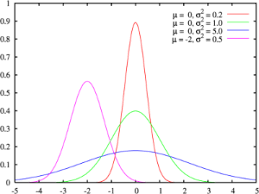
These three posteriors and the prior are illustrated in Figure 1.5.

贝叶斯分析代考

统计代写|贝叶斯分析代写Bayesian Analysis代考|The posterior distribution

贝叶斯推理需要确定后验概率分布θ. 这个任务相当于找到后验pdfθ，这可以使用等式完成

F(θ∣是)=F(θ)F(是∣θ)F(是).
这里，F(是)是的无条件（或先验）pdf是，如给出F(是)=∫F(是∣θ)dF(θ)={∫θF(θ)F(是∣θ)dθ 如果 θ 是连续的 ∑θF(θ)F(是∣θ) 如果 θ 是离散的。
注意：这里，∫F(是∣θ)dF(θ)是 Lebesgue-Stieltjes 积分，在以下情况下可能需要通过将积分分成两部分来评估θ具有混合分布。在连续情况下，考虑dF(θ)作为dF(θ)dθdθ=F(θ)dθ

考虑六个具有以下属性的加载骰子。模具 A 有概率0.1出现 6，骰子 B 和 C 中的每一个都有概率0.2出现 6，骰子 D、E 和 F 中的每一个都有概率0.3即将来临6.
从六个骰子中随机选择一个骰子并掷两次。在这两种情况下，都会出现 6。

什么是后验概率分布θ, 6 出现在所选骰子上的概率。

统计代写|贝叶斯分析代写Bayesian Analysis代考|The proportionality formula

请注意F(是)是一个常数θ在贝叶斯方程中

F(θ∣是)=F(θ)F(是∣θ)/F(是),
这意味着我们也可以将方程写为

F(θ∣是)=F(θ)F(是∣θ)ķ
或作为

F(θ∣是)=CF(θ)F(是∣θ),
在哪里ķ=F(是)和C=1/ķ.
我们也可以写

F(θ∣是)∝F(θ)F(是∣θ),
在哪里∝是比例符号。

等效地，我们可以写

F(θ∣是)θ∝F(θ)F(是∣θ)
强调相称性是专门针对θ.
表达最后一个方程的另一种方法是

F(θ∣是)∝F(θ)×大号(θ∣是),
在哪里大号(θ∣是)是似然函数（定义为模型密度F(是∣θ)乘以任何常数关于θ，并被视为一个函数θ而不是是）。
最后一个方程也可以用文字表述为：
后验与先验时间成正比。
这些观察结果表明了一种确定所需后验分布的快捷方法，无需计算F(是)（这可能很困难）。

该方法是将先验密度（或该密度的核）乘以似然函数，并尝试识别结果函数θ作为众所周知或常见分布的密度。
一旦确定了后验分布，F(是)然后可以很容易地获得相关的归一化常数。

统计代写|贝叶斯分析代写Bayesian Analysis代考|Continuous parameters

上面的例子都有一个离散的目标参数。以下示例说明了涉及连续参数的贝叶斯推理。这种情况没有出现新问题，只是参数的先验密度和后验密度可能不再直接解释为概率。

考虑以下贝叶斯模型：

(是∣θ)∼二项式⁡(n,θ) θ∼贝塔⁡(一个,b) （事先的）。
求后验分布θ.
运动解决方案1.8
后验密度为

F(θ∣是)∝F(θ)F(是∣θ) =θ一个−1(1−θ)b−1乙(一个,b)×(n 是)θ是(1−θ)n−是 ∝θ一个−1(1−θ)b−1×θ是(1−θ)n−是（忽略常数 =θ(一个+是)−1(1−θ)(b+n−是)−1,0<θ<1
这是带有参数的 beta 密度的内核一个+是和b+n−是. 由此可知，后验分布θ是（谁）给的

(θ∣是)∼贝塔⁡(一个+是,b+n−是),
和后验密度θ是（准确地）

F(θ∣是)=θ(一个+是)−1(1−θ)(b+n−是)−1乙(一个+是,b+n−是),0<θ<1.
例如，假设一个=b=1，那是，θ∼乙和吨一个(1,1).
那么先验密度是F(θ)=θ1−1(1−θ)1−1乙(1,1)=1,0<θ<1.
因此先验也可以写成θ∼在(0,1).
另外，假设n=2. 那么有三个可能的值是，即 0,1 和 2 ，它们分别导致以下三个后验：

(θ∣是)∼贝塔⁡(1+0,1+2−0)=贝塔⁡(1,3) (θ∣是)∼贝塔⁡(1+1,1+2−1)=贝塔⁡(2,2) (θ∣是)∼贝塔⁡(1+2,1+2−2)=贝塔⁡(3,1)
这三个后验和先验如图 1.5 所示。

统计代写|贝叶斯分析代写Bayesian Analysis代考请认准statistics-lab™

统计代写请认准statistics-lab™. statistics-lab™为您的留学生涯保驾护航。

金融工程代写

金融工程是使用数学技术来解决金融问题。金融工程使用计算机科学、统计学、经济学和应用数学领域的工具和知识来解决当前的金融问题，以及设计新的和创新的金融产品。

非参数统计代写

非参数统计指的是一种统计方法，其中不假设数据来自于由少数参数决定的规定模型；这种模型的例子包括正态分布模型和线性回归模型。

广义线性模型代考

广义线性模型（GLM）归属统计学领域，是一种应用灵活的线性回归模型。该模型允许因变量的偏差分布有除了正态分布之外的其它分布。

术语广义线性模型（GLM）通常是指给定连续和/或分类预测因素的连续响应变量的常规线性回归模型。它包括多元线性回归，以及方差分析和方差分析（仅含固定效应）。

有限元方法代写

有限元方法（FEM）是一种流行的方法，用于数值解决工程和数学建模中出现的微分方程。典型的问题领域包括结构分析、传热、流体流动、质量运输和电磁势等传统领域。

有限元是一种通用的数值方法，用于解决两个或三个空间变量的偏微分方程（即一些边界值问题）。为了解决一个问题，有限元将一个大系统细分为更小、更简单的部分，称为有限元。这是通过在空间维度上的特定空间离散化来实现的，它是通过构建对象的网格来实现的：用于求解的数值域，它有有限数量的点。边界值问题的有限元方法表述最终导致一个代数方程组。该方法在域上对未知函数进行逼近。[1] 然后将模拟这些有限元的简单方程组合成一个更大的方程系统，以模拟整个问题。然后，有限元通过变化微积分使相关的误差函数最小化来逼近一个解决方案。

tatistics-lab作为专业的留学生服务机构，多年来已为美国、英国、加拿大、澳洲等留学热门地的学生提供专业的学术服务，包括但不限于Essay代写，Assignment代写，Dissertation代写，Report代写，小组作业代写，Proposal代写，Paper代写，Presentation代写，计算机作业代写，论文修改和润色，网课代做，exam代考等等。写作范围涵盖高中，本科，研究生等海外留学全阶段，辐射金融，经济学，会计学，审计学，管理学等全球99%专业科目。写作团队既有专业英语母语作者，也有海外名校硕博留学生，每位写作老师都拥有过硬的语言能力，专业的学科背景和学术写作经验。我们承诺100%原创，100%专业，100%准时，100%满意。

随机分析代写

随机微积分是数学的一个分支，对随机过程进行操作。它允许为随机过程的积分定义一个关于随机过程的一致的积分理论。这个领域是由日本数学家伊藤清在第二次世界大战期间创建并开始的。

时间序列分析代写

随机过程，是依赖于参数的一组随机变量的全体，参数通常是时间。随机变量是随机现象的数量表现，其时间序列是一组按照时间发生先后顺序进行排列的数据点序列。通常一组时间序列的时间间隔为一恒定值（如1秒，5分钟，12小时，7天，1年），因此时间序列可以作为离散时间数据进行分析处理。研究时间序列数据的意义在于现实中，往往需要研究某个事物其随时间发展变化的规律。这就需要通过研究该事物过去发展的历史记录，以得到其自身发展的规律。

回归分析代写

多元回归分析渐进（Multiple Regression Analysis Asymptotics）属于计量经济学领域，主要是一种数学上的统计分析方法，可以分析复杂情况下各影响因素的数学关系，在自然科学、社会和经济学等多个领域内应用广泛。

MATLAB代写

MATLAB 是一种用于技术计算的高性能语言。它将计算、可视化和编程集成在一个易于使用的环境中，其中问题和解决方案以熟悉的数学符号表示。典型用途包括：数学和计算算法开发建模、仿真和原型制作数据分析、探索和可视化科学和工程图形应用程序开发，包括图形用户界面构建MATLAB 是一个交互式系统，其基本数据元素是一个不需要维度的数组。这使您可以解决许多技术计算问题，尤其是那些具有矩阵和向量公式的问题，而只需用 C 或 Fortran 等标量非交互式语言编写程序所需的时间的一小部分。MATLAB 名称代表矩阵实验室。MATLAB 最初的编写目的是提供对由 LINPACK 和 EISPACK 项目开发的矩阵软件的轻松访问，这两个项目共同代表了矩阵计算软件的最新技术。MATLAB 经过多年的发展，得到了许多用户的投入。在大学环境中，它是数学、工程和科学入门和高级课程的标准教学工具。在工业领域，MATLAB 是高效研究、开发和分析的首选工具。MATLAB 具有一系列称为工具箱的特定于应用程序的解决方案。对于大多数 MATLAB 用户来说非常重要，工具箱允许您学习和应用专业技术。工具箱是 MATLAB 函数（M 文件）的综合集合，可扩展 MATLAB 环境以解决特定类别的问题。可用工具箱的领域包括信号处理、控制系统、神经网络、模糊逻辑、小波、仿真等。

R语言代写	问卷设计与分析代写
PYTHON代写	回归分析与线性模型代写
MATLAB代写	方差分析与试验设计代写
STATA代写	机器学习/统计学习代写
SPSS代写	计量经济学代写
EVIEWS代写	时间序列分析代写
EXCEL代写	深度学习代写
SQL代写	各种数据建模与可视化代写

统计代写|贝叶斯分析代写Bayesian Analysis代考|Bayesian Basics

Posted on 2022年6月21日2022年6月21日 by statistics-lab

如果你也在怎样代写贝叶斯分析Bayesian Analysis这个学科遇到相关的难题，请随时右上角联系我们的24/7代写客服。

我们提供的贝叶斯分析Bayesian Analysis及其相关学科的代写，服务范围广, 其中包括但不限于:

Statistical Inference 统计推断
Statistical Computing 统计计算
Advanced Probability Theory 高等概率论
Advanced Mathematical Statistics 高等数理统计学
(Generalized) Linear Models 广义线性模型
Statistical Machine Learning 统计机器学习
Longitudinal Data Analysis 纵向数据分析
Foundations of Data Science 数据科学基础

统计代写|贝叶斯分析代写Bayesian Analysis代考|Bayesian Basics

统计代写|贝叶斯分析代写Bayesian Analysis代考|Bayes’ rule

The starting point for Bayesian inference is Bayes’ rule. The simplest form of this is
$$
P(A \mid B)=\frac{P(A) P(B \mid A)}{P(A) P(B \mid A)+P(\bar{A}) P(B \mid \bar{A})},
$$
where $A$ and $B$ are events such that $P(B)>0$. This is easily proven by considering that:
$P(A \mid B)=\frac{P(A B)}{P(B)}$ by the definition of conditional probability $P(A B)=P(A) P(B \mid A) \quad$ by the multiplicative law of probability $P(B)=P(A B)+P(\bar{A} B)=P(A) P(B \mid A)+P(\bar{A}) P(B \mid \bar{A})$
by the law of total probability.
We see that the posterior probability $P(A \mid B)$ is equal to the prior probability $P(A)$ multiplied by a factor, where this factor is given by $P(B \mid A) / P(B)$

As regards terminology, we call $P(A)$ the prior probability of $A$ (meaning the probability of $A$ before $B$ is known to have occurred), and we call $P(A \mid B)$ the posterior probability of $A$ given $B$ (meaning the probability of $A$ after $B$ is known to have occurred). We may also say that $P(A)$ represents our a priori beliefs regarding $A$, and $P(A \mid B)$ represents our a posteriori beliefs regarding $A$.

统计代写|贝叶斯分析代写Bayesian Analysis代考|Bayes factors

One way to perform hypothesis testing in the Bayesian framework is via the theory of Bayes factors. Suppose that on the basis of an observed event $D$ (standing for data) we wish to test a null hypothesis
$$
H_{0}: E_{0}
$$
versus an alternative hypothesis
$$
H_{1}: E_{1} \text {, }
$$
where $E_{0}$ and $E_{1}$ are two events (which are not necessarily mutually exclusive or even exhaustive of the event space).
Then we calculate:
$\pi_{0}=P\left(E_{0}\right)=$ the prior probability of the null hypothesis
$\pi_{1}=P\left(E_{1}\right)=$ the prior probability of the alternative hypothesis
$P R O=\pi_{0} / \pi_{1}=$ the prior odds in favour of the null hypothesis
$p_{0}=P\left(E_{0} \mid D\right)=$ the posterior probability of the null hypothesis
$p_{1}=P\left(E_{1} \mid D\right)=$ the posterior probability of the alternative hypothesis
$P O O=p_{0} / p_{1}=$ the posterior odds in favour of the null hypothesis.
The Bayes factor is then defined as $B F=P O O / P R O$. This may be interpreted as the factor by which the data have multiplied the odds in favour of the null hypothesis relative to the alternative hypothesis. If $B F>1$ then the data has increased the relative likelihood of the null, and if $B F<1$ then the data has decreased that relative likelihood. The magnitude of $B F$ tells us how much effect the data has had on the relative likelihood.

统计代写|贝叶斯分析代写Bayesian Analysis代考|Bayesian models

Bayes’ formula extends naturally to statistical models. A Bayesian model is a parametric model in the classical (or frequentist) sense, but with the addition of a prior probability distribution for the model parameter, which is treated as a random variable rather than an unknown constant. The basic components of a Bayesian model may be listed as:

the data, denoted by $y$
the parameter, denoted by $\theta$
the model distribution, given by a specification of $f(y \mid \theta)$ or $F(y \mid \theta)$ or the distribution of $(y \mid \theta)$
the prior distribution, given by a specification of $f(\theta)$ or $F(\theta)$ or the distribution of $\theta .$
Here, $F$ is a generic symbol which denotes cumulative distribution function (cdf), and $f$ is a generic symbol which denotes probability density function (pdf) (when applied to a continuous random variable) or probability mass function (pmf) (when applied to a discrete random variable). For simplicity, we will avoid the term pmf and use the term pdf or density for all types of random variable, including the mixed type.
Note 1: A mixed distribution is defined by a cdf which exhibits at least one discontinuity (or jump) and is strictly increasing over at least one interval of values.

Note 2: The prior may be specified by writing a statement of the form ‘ $\theta \sim \ldots$, where the symbol ‘ $\sim$ ‘ means ‘is distributed as’, and where ‘…’denotes the relevant distribution. Likewise, the model for the data may be specified by writing a statement of the form ‘ $(y \mid \theta) \sim \ldots$ ‘.

Note 3: At this stage we will not usually distinguish between $y$ as a random variable and $y$ as a value of that random variable; but sometimes we may use $Y$ for the former. Each of $y$ and $\theta$ may be a scalar, vector, matrix or array. Also, each component of $y$ and $\theta$ may have a discrete distribution, a continuous distribution, or a mixed distribution.

In the first few examples below, we will focus on the simplest case where both $y$ and $\theta$ are scalar and discrete.

贝叶斯分析代考

统计代写|贝叶斯分析代写Bayesian Analysis代考|Bayes’ rule

贝叶斯推理的起点是贝叶斯规则。最简单的形式是

磷(一个∣乙)=磷(一个)磷(乙∣一个)磷(一个)磷(乙∣一个)+磷(一个¯)磷(乙∣一个¯),
在哪里一个和乙是这样的事件磷(乙)>0. 考虑到这一点，这很容易证明：
磷(一个∣乙)=磷(一个乙)磷(乙)根据条件概率的定义磷(一个乙)=磷(一个)磷(乙∣一个)根据乘法概率定律磷(乙)=磷(一个乙)+磷(一个¯乙)=磷(一个)磷(乙∣一个)+磷(一个¯)磷(乙∣一个¯)
根据全概率定律。
我们看到后验概率磷(一个∣乙)等于先验概率磷(一个)乘以一个因子，该因子由下式给出磷(乙∣一个)/磷(乙)

关于术语，我们称磷(一个)先验概率一个（意思是概率一个前乙已知已经发生），我们称磷(一个∣乙)的后验概率一个给定乙（意思是概率一个后乙已知发生）。我们也可以说磷(一个)代表我们的先验信念一个，和磷(一个∣乙)代表我们关于后验的信念一个.

统计代写|贝叶斯分析代写Bayesian Analysis代考|Bayes factors

在贝叶斯框架中执行假设检验的一种方法是通过贝叶斯因子理论。假设基于观察到的事件D（代表数据）我们希望检验零假设

H0:和0
与替代假设

H1:和1,
在哪里和0和和1是两个事件（它们不一定是相互排斥的，甚至不一定是事件空间的穷举）。
然后我们计算：
圆周率0=磷(和0)=原假设的先验概率
圆周率1=磷(和1)=备择假设的先验概率
磷R○=圆周率0/圆周率1=支持原假设的先验几率
p0=磷(和0∣D)=原假设的后验概率
p1=磷(和1∣D)=备择假设的后验概率
磷○○=p0/p1=支持原假设的后验概率。
贝叶斯因子然后定义为乙F=磷○○/磷R○. 这可以解释为数据乘以有利于零假设相对于备择假设的几率的因素。如果乙F>1那么数据增加了空值的相对可能性，如果乙F<1那么数据降低了这种相对可能性。的幅度乙F告诉我们数据对相对可能性的影响有多大。

统计代写|贝叶斯分析代写Bayesian Analysis代考|Bayesian models

贝叶斯公式自然地扩展到统计模型。贝叶斯模型是经典（或常客）意义上的参数模型，但增加了模型参数的先验概率分布，将其视为随机变量而不是未知常数。贝叶斯模型的基本组成部分可以列出如下：

数据，表示为是
参数，表示为θ
模型分布，由规范给出F(是∣θ)或者F(是∣θ)或分布(是∣θ)
先验分布，由规范给出F(θ)或者F(θ)或分布θ.
这里，F是表示累积分布函数 (cdf) 的通用符号，并且F是一个通用符号，表示概率密度函数 (pdf)（当应用于连续随机变量时）或概率质量函数 (pmf)（当应用于离散随机变量时）。为简单起见，我们将避免使用术语 pmf 并使用术语 pdf 或密度来表示所有类型的随机变量，包括混合类型。
注 1：混合分布由 cdf 定义，该 cdf 表现出至少一个不连续性（或跳跃）并且在至少一个值区间内严格增加。

注 2：先验可以通过编写形式为 ‘θ∼…, 其中符号 ‘∼’ 表示“分布为”，其中“……”表示相关分布。同样，数据的模型可以通过编写形式为 ‘(是∣θ)∼… ‘.

注3：在这个阶段我们通常不会区分是作为随机变量和是作为该随机变量的值；但有时我们可能会使用是对于前者。每一个是和θ可以是标量、向量、矩阵或数组。此外，每个组件是和θ可能具有离散分布、连续分布或混合分布。

在下面的前几个示例中，我们将关注最简单的情况，其中是和θ是标量和离散的。

统计代写请认准statistics-lab™. statistics-lab™为您的留学生涯保驾护航。

金融工程代写

非参数统计代写

非参数统计指的是一种统计方法，其中不假设数据来自于由少数参数决定的规定模型；这种模型的例子包括正态分布模型和线性回归模型。

广义线性模型代考

广义线性模型（GLM）归属统计学领域，是一种应用灵活的线性回归模型。该模型允许因变量的偏差分布有除了正态分布之外的其它分布。

有限元方法代写

随机分析代写

时间序列分析代写

回归分析代写

MATLAB代写

R语言代写	问卷设计与分析代写
PYTHON代写	回归分析与线性模型代写
MATLAB代写	方差分析与试验设计代写
STATA代写	机器学习/统计学习代写
SPSS代写	计量经济学代写
EVIEWS代写	时间序列分析代写
EXCEL代写	深度学习代写
SQL代写	各种数据建模与可视化代写

统计代写|贝叶斯分析代写Bayesian Analysis代考|Preliminary Considerations for Time Series

Posted on 2022年6月6日2022年6月6日 by statistics-lab

如果你也在怎样代写贝叶斯分析Bayesian Analysis这个学科遇到相关的难题，请随时右上角联系我们的24/7代写客服。

我们提供的贝叶斯分析Bayesian Analysis及其相关学科的代写，服务范围广, 其中包括但不限于:

Statistical Inference 统计推断
Statistical Computing 统计计算
Advanced Probability Theory 高等概率论
Advanced Mathematical Statistics 高等数理统计学
(Generalized) Linear Models 广义线性模型
Statistical Machine Learning 统计机器学习
Longitudinal Data Analysis 纵向数据分析
Foundations of Data Science 数据科学基础

统计代写|贝叶斯分析代写Bayesian Analysis代考|Preliminary Considerations for Time Series

统计代写|贝叶斯分析代写Bayesian Analysis代考|Time Series

This chapter initiates the study of time series by presenting the necessary concepts that are essential for a good understanding of the subject. It begins with several examples of time series followed by techniques that will allow the investigator to understand the general characteristics of a time series. The first technique is to discern the general appearance of the series using plotting procedures, then from the plot form a subjective opinion of the trend of the series. More formal procedures using $R$ will reveal the various components (e.g., trend and seasonality) of the series. Based on the knowledge of the general appearance of the series, it allows one to propose a tentative model and see how well it fits the series. After a series of diagnostic checks, a final model is selected. Several examples of time series are now presented to illustrate the process of selecting a final model.

统计代写|贝叶斯分析代写Bayesian Analysis代考|Airline Passenger Bookings

According to Cowpertwait and Metcalfe, the following $\mathrm{R}$ code will reveal the international airline booking, in thousands per month, for the airline Pan Am. This monthly information is also available from the Federal Aviation Administration for the years 1949-1960. See Table $3.1$
RC 3.1.
Data(Air Passengers)
$\mathrm{AP}<-$ Air Passengers
$A P$
The following $\mathrm{R}$ command summary provides the basic statistical characteristics (minimum, maximum, first and third quartiles, mean, and median) of the Air Passenger bookings.

summary (AP)

All information in $\mathrm{R}$ is stored in objects, and in this example, the object is class ts (time series), given by the following command:
class(AP)
[1] “ts”/.
It will be interesting to begin the analysis of this data set by determining its trend and by plotting the data.

统计代写|贝叶斯分析代写Bayesian Analysis代考|Sunspot Data

The book by Feigelson and $B a b u^{2}$ is an excellent book on the use of statistics in astronomy. For the second example, one of the most interesting time series is the sunspot data.

The 1749 sunspot numbers are shown below, but for the total dataset, the link will provide the sunspot data and the corresponding plot of this interesting series.
http://solarscience.msfc.nasa.gov/SunspotCycle.shtml.
The numbers tabulated in SN_m_tot_V2.0.txt are the monthly averages of the daily sunspot number with error estimates as posted at the WDCSILSO, Royal Observatory of Belgium, Brussels.

$$
\begin{array}{llllll}
1749 & 01 & 1749.042 & 96.7 & -1.0 & -1 \
1749 & 02 & 1749.123 & 104.3 & -1.0 & -1 \
1749 & 03 & 1749.204 & 116.7 & -1.0 & -1 \
1749 & 04 & 1749.288 & 92.8 & -1.0 & -1 \
1749 & 05 & 1749.371 & 141.7 & -1.0 & -1 \
1749 & 06 & 1749.455 & 139.2 & -1.0 & -1 \
1749 & 07 & 1749.538 & 158.0 & -1.0 & -1 \
1749 & 08 & 1749.623 & 110.5 & -1.0 & -1 \
1749 & 09 & 1749.707 & 126.5 & -1.0 & -1 \
\ldots . . & &
\end{array}
$$
Ancient Chinese astronomers as well as Galileo discovered that the sun has small dark spots that emerge on one side and disappear on the other side of the sun as it rotates. The period of this time series is approximately 30 days. According to the famous astronomer George Hale, the sunspots depend on the intensity of magnetic fields appearing on the surface of the sun. Now there is a branch of astronomy that is devoted to the solar physics that studies the morphology, evolution, and implications of these active solar areas. What is observable as a consequence of sunspot are solar flares which produce energetic particles and ionic phenomena that are not seen over most of the surface of the sun. Such flares can be disturbing in that they can have a major impact on the weather and on early communication systems. The number of spots observed on the sun and averaged over a month reveals a time series that has a large amplitude with obvious seasonality with a period of approximately 11 years. Refer to Feigelson and Babu , Pp. $422-423$ for a more detailed analysis of sunspot data. The fundamental characteristics (amplitudes, period, and harmonic components) of the sunspot cycle will be obvious from plotting the data.

贝叶斯分析代考

统计代写|贝叶斯分析代写Bayesian Analysis代考|Time Series

本章通过介绍对很好理解该主题至关重要的必要概念来启动时间序列的研究。它从几个时间序列的例子开始，然后是使调查人员能够理解时间序列的一般特征的技术。第一种技术是通过绘图程序识别系列的总体外观，然后从情节形成对系列趋势的主观意见。更正式的程序使用R将揭示该系列的各种组成部分（例如，趋势和季节性）。基于对系列总体外观的了解，它允许人们提出一个暂定模型，并查看它与系列的匹配程度。经过一系列诊断检查后，选择了最终模型。现在给出几个时间序列的例子来说明选择最终模型的过程。

统计代写|贝叶斯分析代写Bayesian Analysis代考|Airline Passenger Bookings

根据 Cowpertwait 和 Metcalfe 的说法，以下R代码将显示泛美航空公司每月数千次的国际航空公司预订。该月度信息也可从联邦航空管理局获得 1949-1960 年。见表3.1
钢筋混凝土 3.1。
数据（航空旅客）
一个磷<−航空旅客
一个磷
以下R命令摘要提供航空旅客预订的基本统计特征（最小值、最大值、第一和第三四分位数、平均值和中位数）。

总结（AP）

中的所有信息R存储在对象中，在此示例中，对象是类 ts（时间序列），由以下命令给出：
class(AP)
[1] “ts”/。
通过确定其趋势和绘制数据来开始分析该数据集将会很有趣。

统计代写|贝叶斯分析代写Bayesian Analysis代考|Sunspot Data

费格尔森的书和乙一个b在2是一本关于在天文学中使用统计数据的优秀书籍。对于第二个示例，最有趣的时间序列之一是太阳黑子数据。

1749 个太阳黑子编号如下所示，但对于整个数据集，该链接将提供太阳黑子数据和这个有趣系列的对应图。
http://solarscience.msfc.nasa.gov/SunspotCycle.shtml。
SN_m_tot_V2.0.txt 中列出的数字是每日太阳黑子数量的月平均值，误差估计值发布在布鲁塞尔比利时皇家天文台 WDCSILSO。

1749011749.04296.7−1.0−1 1749021749.123104.3−1.0−1 1749031749.204116.7−1.0−1 1749041749.28892.8−1.0−1 1749051749.371141.7−1.0−1 1749061749.455139.2−1.0−1 1749071749.538158.0−1.0−1 1749081749.623110.5−1.0−1 1749091749.707126.5−1.0−1 …..
中国古代天文学家和伽利略发现太阳有小黑点，当它旋转时，太阳的一侧出现并在另一侧消失。该时间序列的周期约为 30 天。根据著名天文学家乔治黑尔的说法，太阳黑子取决于太阳表面出现的磁场强度。现在有一个天文学分支专门研究太阳物理学，研究这些活跃的太阳区域的形态、演化和影响。作为太阳黑子的结果，可以观察到的是太阳耀斑，它会产生在太阳大部分表面上看不到的高能粒子和离子现象。这种耀斑可能会令人不安，因为它们会对天气和早期通信系统产生重大影响。在太阳上观察到的平均一个多月的光点数量揭示了一个幅度较大、季节性明显的时间序列，周期约为 11 年。请参阅 Feigelson 和 Babu，Pp。422−423对太阳黑子数据进行更详细的分析。通过绘制数据，太阳黑子周期的基本特征（幅度、周期和谐波分量）将是显而易见的。

统计代写请认准statistics-lab™. statistics-lab™为您的留学生涯保驾护航。

金融工程代写

非参数统计代写

非参数统计指的是一种统计方法，其中不假设数据来自于由少数参数决定的规定模型；这种模型的例子包括正态分布模型和线性回归模型。

广义线性模型代考

广义线性模型（GLM）归属统计学领域，是一种应用灵活的线性回归模型。该模型允许因变量的偏差分布有除了正态分布之外的其它分布。

有限元方法代写

随机分析代写

时间序列分析代写

回归分析代写

MATLAB代写

R语言代写	问卷设计与分析代写
PYTHON代写	回归分析与线性模型代写
MATLAB代写	方差分析与试验设计代写
STATA代写	机器学习/统计学习代写
SPSS代写	计量经济学代写
EVIEWS代写	时间序列分析代写
EXCEL代写	深度学习代写
SQL代写	各种数据建模与可视化代写

统计代写|贝叶斯分析代写Bayesian Analysis代考|Computing

Posted on 2022年6月6日2022年6月6日 by statistics-lab

如果你也在怎样代写贝叶斯分析Bayesian Analysis这个学科遇到相关的难题，请随时右上角联系我们的24/7代写客服。

我们提供的贝叶斯分析Bayesian Analysis及其相关学科的代写，服务范围广, 其中包括但不限于:

Statistical Inference 统计推断
Statistical Computing 统计计算
Advanced Probability Theory 高等概率论
Advanced Mathematical Statistics 高等数理统计学
(Generalized) Linear Models 广义线性模型
Statistical Machine Learning 统计机器学习
Longitudinal Data Analysis 纵向数据分析
Foundations of Data Science 数据科学基础

统计代写|贝叶斯分析代写Bayesian Analysis代考|Computing

统计代写|贝叶斯分析代写Bayesian Analysis代考|Monte-Carlo-Markov Chain

MCMC techniques are especially useful when analyzing data with complex statistical models. For example, when considering a hierarchical model with many levels of parameters, it is more efficient to use a MCMC technique such as Metropolis-Hasting or Gibbs sampling iterative procedure in order to sample from the many posterior distributions. It is very difficult, if not impossible, to use non-iterative direct methods for complex models.

A way to draw samples from a target posterior density $\xi(\theta \mid \mathbf{x})$ is to use Markov chain techniques, where each sample only depends on the last sample drawn. Starting with an approximate target density, the approximations are improved with each step of the sequential procedure. Or in other words, the sequence of samples is converging to samples drawn at random from the target distribution. A random walk from a Markov chain is simulated, where the stationary distribution of the chain is the target density, and the simulated values converge to the stationary distribution or the target density. The main concept in a Markov chain simulation is to devise a Markov process whose stationary distribution is the target density. The simulation must be long enough so that the present samples are close enough to the target. It has been shown that this is possible and that convergence can be accomplished. The general scheme for a Markov chain simulation is to create a sequence $\theta_{t}, t=1,2, \ldots$ by beginning at some value $\theta_{0}$, and at the $t$-th stage, select the present value from a transition function $Q_{t}\left(\theta_{t} \mid \theta_{t-1}\right)$, where the present value $\theta_{t}$ only depends on the previous one, via the transition function. The value of the starting value $\theta_{0}$ is usually based on a good approximation to the target density. In order to converge to the target distribution, the transition function must be selected with care. The account given here is a summary of Gelman et al., 19 , ch. 11 who presents a very complete account of MCMC. Metropolis-Hasting is the general name given to methods of choosing appropriate transition functions, and two special cases of this are the Metropolis algorithm and the other is referred to as Gibbs sampling.

统计代写|贝叶斯分析代写Bayesian Analysis代考|The Metropolis Algorithm

Suppose the target density $\xi(\theta \mid x)$ can be computed, then the Metropolis technique generates a sequence $\theta_{t}, t=1,2, \ldots$ with a distribution that converges to a stationary distribution of the chain. Briefly, the steps taken to construct the sequence are:
a. Draw the initial value $\theta_{0}$ from some approximation to the target density,
b. For $t=1,2, \ldots$ generate a sample $\theta_{}$ from the jumping distribution $G_{t}\left(\theta_{} \mid \theta_{t-1}\right)$,
c. Calculate the ratio $\mathrm{s}=\xi\left(\theta_{} \mid \mathrm{X}\right) \xi\left(\theta_{t-1} \mid \mathrm{X}\right)$ and d. Let $\theta_{t}=\theta_{s}$ with probability $\min (s, 1)$ or let $\theta_{t}=\theta_{t-1}$. To summarize the above, if the jump given by b above increases the posterior density, let $\theta_{t}=\theta_{}$; however, if the jump decreases the posterior density, let $\theta_{t}=\theta_{*}$ with probability s, otherwise let $\theta_{t}=\theta_{t-1}$. One must show the sequence generated is a Markov chain with a unique stationary density that converges to the target distribution. For more information, see Gelman et al. 19 , p. 325

统计代写|贝叶斯分析代写Bayesian Analysis代考|Gibbs Sampling

Another MCMC algorithm is Gibbs sampling that is quite useful for multidimensional problems and is an alternating conditional sampling way to generate samples from the joint posterior distribution. Gibbs sampling can be thought of as a practical way to implement the fact that the joint distribution of two random variables is determined by the two conditional distributions.

The two-variable case is first considered by starting with a pair $\left(\theta_{1}, \theta_{2}\right)$ of random variables. The Gibbs sampler generates a random sample from the joint distribution of $\theta_{1}$ and $\theta_{2}$ by sampling from the conditional distributions of $\theta_{1}$ given $\theta_{2}$ and from $\theta_{2}$ given $\theta_{1}$. The Gibbs sequence of size $k$

$$
\theta_{2}^{0}, \theta_{1}^{0} ; \theta_{2}^{1}, \theta_{1}^{1} ; \theta_{2}^{2}, \theta_{1}^{2} ; \ldots ; \theta_{2}^{k}, \theta_{1}^{k}
$$
is generated by first choosing the initial values $\theta_{2}^{0}, \theta_{1}^{0}$ while the remaining are obtained iteratively by alternating values from the two conditional distributions. Under quite general conditions, for large enough $k$, the final two values $\theta_{2}^{k}, \theta_{1}^{k}$ are samples from their respective marginal distributions. To generate a random sample of size $n$ from the joint posterior distribution, generate the above Gibbs sequence $n$ times. Having generated values from the marginal distributions with large $k$ and $n$, the sample mean and variance will converge to the corresponding mean and variance of the posterior distribution of $\left(\theta_{1}, \theta_{2}\right)$.

Gibbs sampling is an example of an MCMC because the generated samples are drawn from the limiting distribution of a 2 by 2 Markov chain. See Casella and George ${ }^{25}$ for a proof that the generated values are indeed values from the appropriate marginal distributions. Of course, Gibbs sequences can be generated from the joint distribution of three, four, and more random variables.

The Gibbs sampling scheme is illustrated with a case of three random variables for the common mean of two normal populations.

贝叶斯分析代考

统计代写|贝叶斯分析代写Bayesian Analysis代考|Monte-Carlo-Markov Chain

MCMC 技术在使用复杂的统计模型分析数据时特别有用。例如，当考虑具有多个参数级别的层次模型时，使用诸如 Metropolis-Hasting 或 Gibbs 采样迭代程序之类的 MCMC 技术来从许多后验分布中进行采样会更有效。对复杂模型使用非迭代直接方法是非常困难的，如果不是不可能的话。

一种从目标后验密度中抽取样本的方法X(θ∣X)是使用马尔可夫链技术，其中每个样本仅依赖于最后抽取的样本。从一个近似的目标密度开始，随着顺序过程的每一步改进近似值。或者换句话说，样本序列正在收敛到从目标分布中随机抽取的样本。模拟来自马尔可夫链的随机游走，其中链的平稳分布是目标密度，模拟值收敛到平稳分布或目标密度。马尔可夫链模拟的主要概念是设计一个马尔可夫过程，其平稳分布是目标密度。模拟必须足够长，以使当前样本足够接近目标。已经证明这是可能的，并且可以实现收敛。θ吨,吨=1,2,…从某个值开始θ0，并且在吨-th 阶段，从转换函数中选择当前值问吨(θ吨∣θ吨−1), 其中现值θ吨只依赖于前一个，通过转换函数。起始值的值θ0通常基于对目标密度的良好近似。为了收敛到目标分布，必须谨慎选择转移函数。此处给出的说明是 Gelman 等人的摘要，第 19 章，第 2 章。11 人提供了一个非常完整的 MCMC 帐户。Metropolis-Hasting 是选择适当转移函数的方法的总称，其中两种特殊情况是 Metropolis 算法，另一种称为 Gibbs 采样。

统计代写|贝叶斯分析代写Bayesian Analysis代考|The Metropolis Algorithm

假设目标密度X(θ∣X)可以计算，然后 Metropolis 技术生成一个序列θ吨,吨=1,2,…具有收敛到链的平稳分布的分布。简而言之，构建序列所采取的步骤是：
a．绘制初始值θ0从某种近似到目标密度，
b。为了吨=1,2,…生成样本θ从跳跃分布G吨(θ∣θ吨−1)，
c。计算比率s=X(θ∣X)X(θ吨−1∣X)和 d。让θ吨=θs有概率分钟(s,1)或让θ吨=θ吨−1. 综上所述，如果上面 b 给出的跳跃增加了后验密度，让θ吨=θ; 然而，如果跳跃降低后验密度，让θ吨=θ∗概率为 s，否则让θ吨=θ吨−1. 必须证明生成的序列是一个马尔可夫链，它具有收敛到目标分布的独特平稳密度。有关详细信息，请参阅 Gelman 等人。19，页。325

统计代写|贝叶斯分析代写Bayesian Analysis代考|Gibbs Sampling

另一种 MCMC 算法是 Gibbs 采样，它对多维问题非常有用，是一种交替的条件采样方式，用于从联合后验分布生成样本。吉布斯抽样可以被认为是实现两个随机变量的联合分布由两个条件分布决定的一种实用方法。

首先考虑从一对开始考虑双变量情况(θ1,θ2)的随机变量。Gibbs 采样器从联合分布中生成随机样本θ1和θ2通过从条件分布中抽样θ1给定θ2并从θ2给定θ1. 大小的吉布斯序列ķ

θ20,θ10;θ21,θ11;θ22,θ12;…;θ2ķ,θ1ķ
通过首先选择初始值生成θ20,θ10而其余的则通过交替来自两个条件分布的值迭代获得。在相当一般的条件下，对于足够大的ķ, 最后两个值θ2ķ,θ1ķ是来自它们各自边缘分布的样本。生成大小的随机样本n从联合后验分布，生成上述吉布斯序列n次。从具有大的边际分布产生的价值ķ和n，样本均值和方差会收敛到对应的后验分布均值和方差(θ1,θ2).

Gibbs 抽样是 MCMC 的一个例子，因为生成的样本是从 2×2 马尔可夫链的极限分布中抽取的。见卡塞拉和乔治25证明生成的值确实是来自适当边际分布的值。当然，吉布斯序列可以从三个、四个和更多随机变量的联合分布中生成。

Gibbs 抽样方案以两个正态总体的共同平均值的三个随机变量为例进行说明。

统计代写请认准statistics-lab™. statistics-lab™为您的留学生涯保驾护航。

金融工程代写

非参数统计代写

非参数统计指的是一种统计方法，其中不假设数据来自于由少数参数决定的规定模型；这种模型的例子包括正态分布模型和线性回归模型。

广义线性模型代考

广义线性模型（GLM）归属统计学领域，是一种应用灵活的线性回归模型。该模型允许因变量的偏差分布有除了正态分布之外的其它分布。

有限元方法代写

随机分析代写

时间序列分析代写

回归分析代写

MATLAB代写

R语言代写	问卷设计与分析代写
PYTHON代写	回归分析与线性模型代写
MATLAB代写	方差分析与试验设计代写
STATA代写	机器学习/统计学习代写
SPSS代写	计量经济学代写
EVIEWS代写	时间序列分析代写
EXCEL代写	深度学习代写
SQL代写	各种数据建模与可视化代写

统计代写|贝叶斯分析代写Bayesian Analysis代考|Predictive Inference

Posted on 2022年6月6日2022年6月6日 by statistics-lab

如果你也在怎样代写贝叶斯分析Bayesian Analysis这个学科遇到相关的难题，请随时右上角联系我们的24/7代写客服。

我们提供的贝叶斯分析Bayesian Analysis及其相关学科的代写，服务范围广, 其中包括但不限于:

Statistical Inference 统计推断
Statistical Computing 统计计算
Advanced Probability Theory 高等概率论
Advanced Mathematical Statistics 高等数理统计学
(Generalized) Linear Models 广义线性模型
Statistical Machine Learning 统计机器学习
Longitudinal Data Analysis 纵向数据分析
Foundations of Data Science 数据科学基础

统计代写|贝叶斯分析代写Bayesian Analysis代考|Predictive Inference

统计代写|贝叶斯分析代写Bayesian Analysis代考|The Binomial Population

Suppose the binomial case is again considered, where the posterior density of the binomial parameter $\theta$ is
$$
\begin{aligned}
\xi(\theta \mid X)=& {[\Gamma(\alpha+\beta) \Gamma(n+1) / \Gamma(\alpha) \Gamma(\beta) \Gamma(x+1) \Gamma(n-x+1)] } \
& \theta^{\alpha+x-1}(1-\theta)^{\beta+n-x-1}
\end{aligned}
$$
a beta with parameters $\alpha+x$ and $n-x+\beta$, and $X$ is the sum of the set of $n$ observations. The population mass function of a future observation $Z$ is

$f(z / \theta)=\theta^{z}(1-\theta)^{1-z}$, and the predictive mass function of $Z$, called the beta-binomial, is
$$
\begin{aligned}
&\mathrm{g}(\mathrm{z} \mid \mathrm{X})=\Gamma(\alpha+\beta) \Gamma(n+1) \Gamma\left(\alpha+\sum_{i=1}^{i=n} x_{i}+z\right) \Gamma(1+n+\beta-x-z) \div \
&\Gamma(\alpha) \Gamma(\beta) \Gamma(n-x+1) \Gamma(x+1) \Gamma(n+1+\alpha+\beta)
\end{aligned}
$$
where $z=0.1$. Note this function does not depend on the unknown parameter, and that the $n$ past observations are known, and that if $\alpha=\beta=1$, one is assuming a uniform prior density for $\theta$.

As an example for the predictive distribution of the binomial distribution, let
$$
\mathrm{N}=\left(\begin{array}{l}
1,7,4,6,2 \
5,3,4,6,5 \
3,6,2,3,1 \
5,7,2,5,4 \
6,1,3,3,4
\end{array}\right)
$$
be the transition counts for a five-state Markov chain and
$$
\Phi=\left(\begin{array}{l}
\phi_{11}, \phi_{12}, \phi_{13}, \phi_{14}, \phi_{15} \
\phi_{21}, \phi_{22}, \phi_{23}, \phi_{24}, \phi_{25} \
\phi_{31}, \phi_{32}, \phi_{33}, \phi_{34}, \phi_{35} \
\phi_{41}, \phi_{42}, \phi_{43}, \phi_{44}, \phi_{45} \
\phi_{51}, \phi_{52}, \phi_{53}, \phi_{54}, \phi_{55}
\end{array}\right)
$$
as the one-step transition matrix.
Our focus is on forecasting the number of transitions $Z_{11}$ from 1 to 1 , that is the number of times the chain remains in state 1 , assuming a total of $m$ replications for the first row of the chain, that is $Z_{11}=0,1,2, \ldots, m$. Using (2.77), one may show the predictive mass function of $Z_{11}$ is equation (2.78)
$$
\begin{gathered}
g\left(z \mid n_{11}=1\right)=\left(\begin{array}{c}
m \
z
\end{array}\right) \Gamma(\alpha+\beta) \Gamma(n+1) \Gamma\left(\alpha+z+n_{11}\right) \Gamma\left(\beta+n-z-n_{11}\right) / \
\Gamma(\alpha) \Gamma(\beta) \Gamma\left(n_{11}+1\right) \Gamma\left(n-n_{11}+1\right) \Gamma(\alpha+\beta+n)
\end{gathered}
$$
The relevant quantities of $(2.78)$ are $n=20, n_{11}=1$. Also remember that $\alpha$ and $\beta$ are the parameters of the prior distribution of $\phi_{11}$, the probability of remaining in state 1 , and that predictive inferences are conditional on $n=20$, the total transition counts for the first row of the one-step transition matrix of the chain.

统计代写|贝叶斯分析代写Bayesian Analysis代考|Introduction

It is imperative to check model adequacy in order to choose an appropriate model and to conduct a valid study. The approach taken here is based on many sources, including Gelman et al., ${ }^{2}$ Carlin and Louis, ${ }^{18}$ and Congdon ${ }^{16} \mathrm{Our}$ main focus will be on the likelihood function of the posterior distribution, and not the prior distribution, and to this end, graphical representations such as histograms, boxplots, and various probability plots of the original observations will be compared with those of the observations generated from the predictive distribution. In addition to graphical methods, Bayesian versions of overall goodness-offit-type operations are taken to check model validity. Methods presented at this juncture are just a small subset of those presented in more advanced works, including Gelman et al., Carlin and Louis, and Congdon.

Of course, the prior distribution is an important component of the analysis, and if one is not sure of the ‘true’ prior, one should perform a sensitivity analysis to determine the robustness of posterior inferences to various alternative choices of prior information. See Gelman et al. or Carlin and Louis for details of performing a sensitivity study for prior information. Our approach is to either use informative or vague prior distributions, where the former is done when prior relevant experimental evidence determines the prior, or the latter is taken if there is none or very little germane experimental studies. In scientific studies, the most likely scenario is that there are relevant experimental studies providing informative prior information.

统计代写|贝叶斯分析代写Bayesian Analysis代考|Sampling from an Exponential, but Assuming a Normal Population

Consider a random sample of size 30 from an exponential distribution with mean 3 . An exponential distribution is often used to model the survival times of a screening test. The 30 exponential values are generated with $B C 2.4$.
BC $2.4$
model;
The sample mean and standard deviation are $4.13$ and $3.739$, respectively.
Assume the sample is from a normal population with unknown mean and variance, with an improper prior density
$\xi(\mu, \tau)=1 / \tau, \mu \in R$ and $\sigma>0$, then the posterior predictive density is a univariatet with $n-1=29$ degrees of freedom, mean $\bar{x}=3.744$, standard deviation $3.872$, and precision $p=.0645$. This is verified from the original observations $x$ and the formula for the precision. From the predictive distribution, 30 observations are generated with BC $2.5$.
BC 2.5.
{
For $(t$ in $1: 30){$
Z[t] $\mathrm{t}(3.744, .0645,29)}$
$\mathrm{z}=(2.76213,3.46370,2.88747,3.13581,4.50398,5.09963,4.39670,3.24032,3.58791$,
$5.60893,3.76411,3.15034,4.15961,2.83306,3.64620,3.48478,2.24699,2.44810$,
$3.39590,3.56703,4.04226,4.00720,4.33006,3.44320,5.03451,2.07679,2.30578$,
$5.99297,3.88463,2.52737)$
which gives a mean of $\bar{z}=3.634$ and standard deviation $S=.975$.
The histograms obviously are different, where for the original observations, a right skewness is depicted; however, this is lacking for the histogram of the predicted observations, which is for a $t$-distribution. Although the example seems trivial, it would not be for the first time that exponential observations were analyzed as if they were generated from a normal population! Of course,

we have seen the relevance of the exponential distribution to Markov jump processes such as the Poisson process of Section 3.4.3, where the inter-arrival times are independent and identically distributed with a mean that is the reciprocal of the mean rate of event happenings.

It would be interesting to generate more replicate samples from the predictive distribution in order to see if these conclusions hold firm.

贝叶斯分析代考

统计代写|贝叶斯分析代写Bayesian Analysis代考|The Binomial Population

假设再次考虑二项式情况，其中二项式参数的后验密度θ是

X(θ∣X)=[Γ(一个+b)Γ(n+1)/Γ(一个)Γ(b)Γ(X+1)Γ(n−X+1)] θ一个+X−1(1−θ)b+n−X−1
带有参数的 beta一个+X和n−X+b，和X是集合的总和n观察。未来观测的总体质量函数从是

F(和/θ)=θ和(1−θ)1−和，以及预测质量函数从，称为 beta-二项式，是

G(和∣X)=Γ(一个+b)Γ(n+1)Γ(一个+∑一世=1一世=nX一世+和)Γ(1+n+b−X−和)÷ Γ(一个)Γ(b)Γ(n−X+1)Γ(X+1)Γ(n+1+一个+b)
在哪里和=0.1. 请注意，此函数不依赖于未知参数，并且n过去的观察是已知的，并且如果一个=b=1，一个假设是均匀的先验密度θ.

作为二项分布的预测分布的一个例子，让

ñ=(1,7,4,6,2 5,3,4,6,5 3,6,2,3,1 5,7,2,5,4 6,1,3,3,4)
是一个五态马尔可夫链的转移计数和

披=(φ11,φ12,φ13,φ14,φ15 φ21,φ22,φ23,φ24,φ25 φ31,φ32,φ33,φ34,φ35 φ41,φ42,φ43,φ44,φ45 φ51,φ52,φ53,φ54,φ55)
作为一步转移矩阵。
我们的重点是预测转换的数量从11从 1 到 1 ，即链保持在状态 1 的次数，假设总共米复制链的第一行，即从11=0,1,2,…,米. 使用 (2.77)，可以显示预测质量函数从11是方程 (2.78)

G(和∣n11=1)=(米和)Γ(一个+b)Γ(n+1)Γ(一个+和+n11)Γ(b+n−和−n11)/ Γ(一个)Γ(b)Γ(n11+1)Γ(n−n11+1)Γ(一个+b+n)
相关数量(2.78)是n=20,n11=1. 还记得一个和b是先验分布的参数φ11, 保持在状态 1 的概率 , 并且预测推论的条件是n=20，链的单步转移矩阵的第一行的总转移计数。

统计代写|贝叶斯分析代写Bayesian Analysis代考|Introduction

为了选择合适的模型并进行有效的研究，必须检查模型的充分性。这里采用的方法基于许多来源，包括 Gelman 等人，2卡林和路易斯，18和康登16○在r主要关注的是后验分布的似然函数，而不是先验分布，为此，原始观测值的直方图、箱线图和各种概率图等图形表示将与生成的观测值进行比较预测分布。除了图形方法外，还采用贝叶斯版本的整体优劣型操作来检查模型的有效性。此时提出的方法只是更高级作品中提出的方法的一小部分，包括 Gelman 等人、Carlin 和 Louis 以及 Congdon。

当然，先验分布是分析的重要组成部分，如果不确定“真实”先验，则应进行敏感性分析，以确定后验推断对各种先验信息选择的稳健性。见 Gelman 等人。或 Carlin 和 Louis，了解对先验信息进行敏感性研究的详细信息。我们的方法是使用信息丰富或模糊的先验分布，其中前者是在先前的相关实验证据确定先验时完成的，或者在没有或很少有密切相关的实验研究时采用后者。在科学研究中，最可能的情况是相关的实验研究提供了丰富的先验信息。

统计代写|贝叶斯分析代写Bayesian Analysis代考|Sampling from an Exponential, but Assuming a Normal Population

考虑来自均值为 3 的指数分布的大小为 30 的随机样本。指数分布通常用于模拟筛选测试的生存时间。生成 30 个指数值乙C2.4.
公元前2.4
模型;
样本均值和标准差为4.13和3.739，分别。
假设样本来自具有未知均值和方差的正态总体，具有不正确的先验密度
X(μ,τ)=1/τ,μ∈R和σ>0, 那么后验预测密度是一个单变量n−1=29自由度，平均值X¯=3.744, 标准差3.872, 和精度p=.0645. 这从原始观察中得到验证X以及精度公式。根据预测分布，使用 BC 生成 30 个观测值2.5.
公元前 2.5。
{
对于(吨在1:30)$从[吨]$吨(3.744,.0645,29)
和=(2.76213,3.46370,2.88747,3.13581,4.50398,5.09963,4.39670,3.24032,3.58791,
5.60893,3.76411,3.15034,4.15961,2.83306,3.64620,3.48478,2.24699,2.44810,
3.39590,3.56703,4.04226,4.00720,4.33006,3.44320,5.03451,2.07679,2.30578,
5.99297,3.88463,2.52737)
这给出了一个平均值和¯=3.634和标准差小号=.975.
直方图显然是不同的，其中对于原始观察，描绘了右偏度；然而，对于预测观测值的直方图来说，这是缺乏的，这是吨-分配。尽管这个例子看起来微不足道，但这并不是第一次将指数观测值分析为好像它们是从正常人群中生成的一样！当然，

我们已经看到了指数分布与马尔可夫跳跃过程的相关性，例如第 3.4.3 节的泊松过程，其中到达间隔时间是独立的并且同分布，平均值是事件发生的平均速率的倒数。

从预测分布中生成更多重复样本以查看这些结论是否成立会很有趣。

统计代写请认准statistics-lab™. statistics-lab™为您的留学生涯保驾护航。

金融工程代写

非参数统计代写

非参数统计指的是一种统计方法，其中不假设数据来自于由少数参数决定的规定模型；这种模型的例子包括正态分布模型和线性回归模型。

广义线性模型代考

广义线性模型（GLM）归属统计学领域，是一种应用灵活的线性回归模型。该模型允许因变量的偏差分布有除了正态分布之外的其它分布。

有限元方法代写

随机分析代写

时间序列分析代写

回归分析代写

MATLAB代写

R语言代写	问卷设计与分析代写
PYTHON代写	回归分析与线性模型代写
MATLAB代写	方差分析与试验设计代写
STATA代写	机器学习/统计学习代写
SPSS代写	计量经济学代写
EVIEWS代写	时间序列分析代写
EXCEL代写	深度学习代写
SQL代写	各种数据建模与可视化代写

统计代写|贝叶斯分析代写Bayesian Analysis代考|Inference

Posted on 2022年6月6日2022年6月6日 by statistics-lab

如果你也在怎样代写贝叶斯分析Bayesian Analysis这个学科遇到相关的难题，请随时右上角联系我们的24/7代写客服。

我们提供的贝叶斯分析Bayesian Analysis及其相关学科的代写，服务范围广, 其中包括但不限于:

Statistical Inference 统计推断
Statistical Computing 统计计算
Advanced Probability Theory 高等概率论
Advanced Mathematical Statistics 高等数理统计学
(Generalized) Linear Models 广义线性模型
Statistical Machine Learning 统计机器学习
Longitudinal Data Analysis 纵向数据分析
Foundations of Data Science 数据科学基础

统计代写|贝叶斯分析代写Bayesian Analysis代考|Inference

统计代写|贝叶斯分析代写Bayesian Analysis代考|Introduction

In a statistical context, by inference, one usually means estimation of parameters, tests of hypotheses, and prediction of future observations. With the Bayesian approach, all inferences are based on the posterior distribution of the parameters, which in turn is based on the sample, via the likelihood function and the prior distribution. We have seen the role of the prior density and likelihood function in determining the posterior distribution, and presently will focus on the determination of point and interval estimation of the model parameters, and later will emphasize how the posterior distribution determines a test of hypothesis. Finally, the role of the predictive distribution in testing hypotheses and in goodness of fit will be explained.

When the model has only one parameter, one would estimate that parameter by listing its characteristics, such as the posterior mean, media, and standard deviation and plotting the posterior density. However, if there are several parameters, one would determine the marginal posterior distribution of the relevant parameters and, as above, calculate its characteristics (e.g., mean, median, mode, standard deviation, etc.) and plot the densities. Interval estimates of the parameters are also usually reported and are called credible intervals.

统计代写|贝叶斯分析代写Bayesian Analysis代考|Estimation

Inferences for the normal $(\mu, \tau)$ population are somewhat more demanding, because both parameters are unknown. Assuming the vague prior density $\xi(\mu, \tau) \propto 1 / \tau$, the marginal posterior distribution of the population mean $\mu$ is a $t$-distribution with $n-1$ degrees of freedom, mean $\bar{x}$, and precision $n / s^{2}$; thus, the mean and the median are the same and provide a natural estimator of $\mu$, and because of the symmetry of the $t$-density, a $(1-\alpha)$ credible interval for $\mu$ is $\bar{x} \pm t_{\alpha / 2, n-1} S / \sqrt{n}$, where $t_{\alpha / 2, n-1}$ is the upper 100 $\alpha / 2$ percent point of the $t$-distribution with $n$-1degrees of freedom. To generate values from the $t\left(n-1, \bar{x}, n / S^{2}\right)$ distribution, generate values from Student’s $t$-distribution with $n-1$ degrees of freedom, multiply each by $S / \sqrt{n}$, and then add $\bar{x}$ to each. Suppose $n-30$,

$$
\begin{aligned}
&x=(7.8902,4.8343,11.0677,8.7969,4.0391,4.0024,6.6494,8.4788,0.7939,5.0689, \
&6.9175,6.1092,8.2463,10.3179,1.8429,3.0789,2.8470,5.1471,6.3730,5.2907,1.5024, \
&3.8193,9.9831,6.2756,5.3620,5.3297,9.3105,6.5555,0.8189,0.4713) \text {, then } \
&\bar{x}=5.57 \text { and } S=2.92
\end{aligned}
$$
Using the same dataset, the following WinBugs code is used to analyze the problem.
BC $2.1$
Model;
${$ for ( i in 1:30) ${x[i] \sim \operatorname{dnorm}(\mathrm{mu}, \mathrm{tau})}$
mu $\sim$ dnorm $(0.0,0001)$
tau $\sim$ dgamma(. $0001, .0001)$
sigma $<-1 /$ tau $}$
list $(\mathrm{x}=\mathrm{c}(7.8902,4.8343,11.0677,8.7969,4.0391,4.0024,6.6494,8.4788,0.7939,5.0689$, $6.9175,6.1092,8.2463,10.3179,1.8429,3.0789,2.8470,5.1471,6.3730,5.2907,1.5024$, $3.8193,9.9831,6.2756,5.3620,5.3297,9.3105,6.5555,0.8189,0.4713))$
$\operatorname{list}(\mathrm{mu}=0, \mathrm{tau}=1)$
Note, that a somewhat different prior was employed here, compared to previously, in that $\mu$ and $\tau$ are independent and assigned properly, but noninformative distributions. The corresponding analysis gives the following as shown in Table 2.2.

Upper and lower refer to the lower and upper $21 / 2$ percent points of the posterior distribution. Note a $95 \%$ credible interval for mu is $(4.47,6.65)$ and the estimation error is $.003566$. See the Appendix for the details on executing the WinBUGS statements above.

The program generated 30,000 samples from the joint posterior distribution of $\mu$ and $\sigma$ using a Gibbs sampling algorithm, and used 29,000 for the posterior moments and graphs, with a refresh of 100 .

统计代写|贝叶斯分析代写Bayesian Analysis代考|Testing Hypotheses

An important feature of inference is testing hypotheses. Often in stochastic processes, the scientific hypothesis can be expressed in statistical terms and

a formal test implemented. Suppose $\Omega=\Omega_{0} \cup \Omega_{1}$ is a partition of the parameter space, then the null hypothesis is designated as $H_{0}: \theta \in \Omega_{0}$ and the alternative by $H_{1}: \theta \in \Omega_{1}$, and a test of $H_{0}$ versus $H_{1}$ consists of rejecting $H_{0}$ in favor of $H_{1}$ if the observations $x=\left(x_{1}, x_{2}, \ldots, x_{n}\right)$ belong to a critical region C. In the usual approach, the critical region is based on the probabilities of type I errors, namely $\mathrm{P}{\mathrm{r}}(C \mid \theta)$, where $\theta \in \Omega{0}$ and of type II errors $1-P_{r}(C \mid \theta)$, where $\theta \in \Omega_{1}$. This approach to testing hypothesis was developed formally by Neyman and Pearson and can be found in many of the standard references, such as Lehmann. ${ }^{20}$ Lee ${ }^{21}$ presents a good elementary introduction to testing and estimation in a Bayesian context.
In the Bayesian approach, the posterior probabilities
$$
p_{0}=\operatorname{Pr}\left(\theta \in \Omega_{0} \mid \text { data }\right)
$$
and
$$
p_{1}=\operatorname{Pr}\left(\theta \in \Omega_{1} \mid \text { data }\right)
$$
are required, and on the basis of the two, a decision is made whether or not to reject $\mathrm{H}$ in favor of $\mathrm{A}$ or to reject $\mathrm{A}$ in favor of $\mathrm{H}$. Also required are the two corresponding prior probabilities
$$
\pi_{0}=\operatorname{Pr}\left(\theta \in \Omega_{0}\right)
$$
and
$$
\pi_{1}=\operatorname{Pr}\left(\theta \in \Omega_{1}\right) .
$$
Now consider the prior odds $\pi_{0} / \pi_{1}$ and posterior odds $p_{0} / p_{1}$. In turn, consider the Bayes factor B in favor of $H_{0}$ relative to $H_{1}$, namely
$$
B=\left(p_{0} / p_{1}\right) /\left(\pi_{0} / \pi_{1}\right)
$$
Then, the posterior probabilities $p_{0}$ and $p_{1}$ can be expressed in terms of the Bayes factor, thus:
$$
p_{0}=1 /\left[1+\left(\pi_{1} / \pi_{1}\right) B^{-1}\right]
$$
and the Bayes factor is interpreted as the odds in favor of $H_{0}$ relative to $H_{1}$ as implied by the information from the data.

When the hypotheses are simple, that is, $\Omega_{0}=\left{\theta_{0}\right}$ and $\Omega_{1}=\left{\theta_{1}\right}$, note that the odds ratio can be expressed as the likelihood ratio.
$$
B=p\left(x \mid \theta_{0}\right) / p\left(x \mid \theta_{1}\right)
$$

贝叶斯分析代考

统计代写|贝叶斯分析代写Bayesian Analysis代考|Introduction

在统计背景下，通过推断，通常意味着对参数的估计、假设的检验和对未来观察的预测。使用贝叶斯方法，所有推论都基于参数的后验分布，而后验分布又基于样本，通过似然函数和先验分布。我们已经看到了先验密度和似然函数在确定后验分布中的作用，现在将重点介绍模型参数的点估计和区间估计的确定，稍后将强调后验分布如何确定假设检验。最后，将解释预测分布在检验假设和拟合优度中的作用。

当模型只有一个参数时，可以通过列出其特征（例如后验均值、中值和标准差）并绘制后验密度来估计该参数。但是，如果有多个参数，则可以确定相关参数的边际后验分布，并如上所述计算其特征（例如，平均值、中值、众数、标准差等）并绘制密度图。通常也会报告参数的区间估计值，称为可信区间。

统计代写|贝叶斯分析代写Bayesian Analysis代考|Estimation

正常的推论(μ,τ)人口的要求更高一些，因为这两个参数都是未知的。假设模糊的先验密度X(μ,τ)∝1/τ, 总体的边际后验分布均值μ是一个吨-分布与n−1自由度，平均值X¯, 和精度n/s2; 因此，平均值和中位数是相同的，并提供了一个自然的估计μ，并且由于对称性吨-密度，一个(1−一个)可信区间μ是X¯±吨一个/2,n−1小号/n，在哪里吨一个/2,n−1是上 100一个/2个百分点吨-分布与n-1 自由度。从吨(n−1,X¯,n/小号2)分布，从学生的吨-分布与n−1自由度，每个乘以小号/n，然后加上X¯每个。认为n−30,

X=(7.8902,4.8343,11.0677,8.7969,4.0391,4.0024,6.6494,8.4788,0.7939,5.0689, 6.9175,6.1092,8.2463,10.3179,1.8429,3.0789,2.8470,5.1471,6.3730,5.2907,1.5024, 3.8193,9.9831,6.2756,5.3620,5.3297,9.3105,6.5555,0.8189,0.4713)，然后 X¯=5.57 和小号=2.92
使用相同的数据集，使用下面的 WinBugs 代码来分析问题。
公元前2.1
模型;
$F○r(一世一世n1:30)$X[一世]∼规范⁡(米在,吨一个在)$米在$∼$dn○r米$(0.0,0001)$吨一个在$∼$dG一个米米一个(.$0001,.0001)$s一世G米一个$<−1/$吨一个在$
列表(X=C(7.8902,4.8343,11.0677,8.7969,4.0391,4.0024,6.6494,8.4788,0.7939,5.0689,6.9175,6.1092,8.2463,10.3179,1.8429,3.0789,2.8470,5.1471,6.3730,5.2907,1.5024,3.8193,9.9831,6.2756,5.3620,5.3297,9.3105,6.5555,0.8189,0.4713))
列表⁡(米在=0,吨一个在=1)
请注意，与以前相比，这里采用了一些不同的先验，因为μ和τ是独立的并被正确分配，但没有信息分布。相应的分析给出如下表2.2所示。

上下分别指上下21/2后验分布的百分点。注意一个95%mu 的可信区间是(4.47,6.65)估计误差为.003566. 有关执行上述 WinBUGS 语句的详细信息，请参阅附录。

该程序从联合后验分布中生成了 30,000 个样本μ和σ使用 Gibbs 采样算法，并使用 29,000 用于后验矩和图，刷新为 100 。

统计代写|贝叶斯分析代写Bayesian Analysis代考|Testing Hypotheses

推理的一个重要特征是检验假设。通常在随机过程中，科学假设可以用统计术语和

实施了正式的测试。认为Ω=Ω0∪Ω1是参数空间的一个分区，则原假设被指定为H0:θ∈Ω0和替代方案H1:θ∈Ω1, 和一个测试H0相对H1包括拒绝H0有利于H1如果观察X=(X1,X2,…,Xn)属于临界区 C。在通常的方法中，临界区是基于 I 类错误的概率，即磷r(C∣θ)，在哪里θ∈Ω0和 II 类错误1−磷r(C∣θ)，在哪里θ∈Ω1. 这种检验假设的方法是由 Neyman 和 Pearson 正式开发的，并且可以在许多标准参考文献中找到，例如 Lehmann。20李21对贝叶斯环境中的测试和估计进行了很好的基本介绍。
在贝叶斯方法中，后验概率

p0=公关⁡(θ∈Ω0∣ 数据 )
和

p1=公关⁡(θ∈Ω1∣ 数据 )
是必需的，并在两者的基础上做出是否拒绝的决定H有利于一个或拒绝一个有利于H. 还需要两个相应的先验概率

圆周率0=公关⁡(θ∈Ω0)
和

圆周率1=公关⁡(θ∈Ω1).
现在考虑之前的赔率圆周率0/圆周率1和后验赔率p0/p1. 反过来，考虑贝叶斯因子 B 有利于H0关系到H1，即

乙=(p0/p1)/(圆周率0/圆周率1)
那么，后验概率p0和p1可以用贝叶斯因子表示，因此：

p0=1/[1+(圆周率1/圆周率1)乙−1]
并且贝叶斯因子被解释为有利于H0关系到H1正如数据中的信息所暗示的那样。

当假设很简单时，即\Omega_{0}=\left{\theta_{0}\right}\Omega_{0}=\left{\theta_{0}\right}和\Omega_{1}=\left{\theta_{1}\right}\Omega_{1}=\left{\theta_{1}\right}，请注意，优势比可以表示为似然比。

乙=p(X∣θ0)/p(X∣θ1)

统计代写请认准statistics-lab™. statistics-lab™为您的留学生涯保驾护航。

金融工程代写

非参数统计代写

非参数统计指的是一种统计方法，其中不假设数据来自于由少数参数决定的规定模型；这种模型的例子包括正态分布模型和线性回归模型。

广义线性模型代考

广义线性模型（GLM）归属统计学领域，是一种应用灵活的线性回归模型。该模型允许因变量的偏差分布有除了正态分布之外的其它分布。

有限元方法代写

随机分析代写

时间序列分析代写

回归分析代写

MATLAB代写

R语言代写	问卷设计与分析代写
PYTHON代写	回归分析与线性模型代写
MATLAB代写	方差分析与试验设计代写
STATA代写	机器学习/统计学习代写
SPSS代写	计量经济学代写
EVIEWS代写	时间序列分析代写
EXCEL代写	深度学习代写
SQL代写	各种数据建模与可视化代写

统计代写|贝叶斯分析代写Bayesian Analysis代考|Posterior Information

Posted on 2022年6月6日2022年6月6日 by statistics-lab

如果你也在怎样代写贝叶斯分析Bayesian Analysis这个学科遇到相关的难题，请随时右上角联系我们的24/7代写客服。

我们提供的贝叶斯分析Bayesian Analysis及其相关学科的代写，服务范围广, 其中包括但不限于:

Statistical Inference 统计推断
Statistical Computing 统计计算
Advanced Probability Theory 高等概率论
Advanced Mathematical Statistics 高等数理统计学
(Generalized) Linear Models 广义线性模型
Statistical Machine Learning 统计机器学习
Longitudinal Data Analysis 纵向数据分析
Foundations of Data Science 数据科学基础

统计代写|贝叶斯分析代写Bayesian Analysis代考|Posterior Information

统计代写|贝叶斯分析代写Bayesian Analysis代考|The Binomial Distribution

The preceding section explains how prior information is expressed in an informative or in a noninformative way. Several examples are given and will be revisited as illustrations for the determination of the posterior distribution of the parameters. Suppose a uniform prior distribution for the transition probability (of the five-state Markov chain) $p_{i j}$ is used. What is the posterior distribution of $p_{i j}$ ?
By Bayes theorem,
$$
f\left(p_{i j} \mid N\right) \propto\left(\begin{array}{c}
n \
n_{i j}
\end{array}\right) p_{i j}^{n_{i j}}\left(1-p_{i j}\right)^{n-n_{i j}}
$$
where $n_{i j}$ is the observed transitions from state $i$ to state $j$ and $n$ is the total cell counts for the five-by-five cell frequency matrix $N$. Of course, this is recognized as a beta $\left(n_{i j}+1, n-n_{i j}+1\right)$ distribution, and the posterior mean is $\left(n_{i j}+1 / n+2\right)$. However, if the Lhoste ${ }^{5}$ prior density (2.4) is used, the posterior distribution of $p_{i j}$ is beta $\left(n_{i j}, n-n_{i j}\right)$ with mean $n_{i j} / n$, which is the usual estimator of $p_{i j}$.

统计代写|贝叶斯分析代写Bayesian Analysis代考|The Normal Distribution

Consider a random sample $\mathrm{X}=\left(x_{1}, x_{2}, \ldots, x_{n}\right)$ of size $n$ from a normal $(\mu, 1 / \tau)$ population, where $\tau=1 / \sigma^{2}$ is the inverse of the variance, and suppose the prior information is vague and the Jeffreys-Lhoste prior $\xi(\mu, \tau) \propto 1 / \tau$ is appropriate, then the posterior density of the parameters is
$$
\xi(\mu, \tau \mid \text { data }) \propto \tau^{n / 2-1} \exp -(\tau / 2)\left[n(\mu-\bar{x})^{2}+\sum_{i=1}^{i=n}\left(x_{i}-\bar{x}\right)^{2}\right]
$$

Using the properties of the gamma density, $\tau$ is eliminated by integrating the joint density with respect to $\tau$ to give
$$
\begin{gathered}
\xi(\mu \mid \text { data }) \propto \
\left{\Gamma(n / 2) n^{1 / 2} /(n-1)^{1 / 2} S \pi^{1 / 2} \Gamma((n-10 / 2)} /\left[1+n(\mu-\bar{x})^{2} /(n-1) S^{2}\right]^{(n-1+1) / 2}\right.
\end{gathered}
$$
which is recognized as a $t$-distribution with $n-1$ degrees of freedom, location $\bar{x}$, and precision $n / S^{2}$. Transforming to $(\mu-\bar{x}) \sqrt{n} / S$, the resulting variable has a Student’s $t$-distribution with $n-1$ degrees of freedom. Note the mean of $\mu$ is the sample mean, while the variance is $[(n-1) / n(n-3)], n>3$.
Eliminating $\mu$ from (12) results in the marginal distribution of $\tau$ as
$$
\xi\left(\tau \mid s^{2}\right) \propto \tau^{[(n-1) / 2 \mid-1} \exp -\tau(n-1) S^{2} / 2, \tau>0,
$$
which is a gamma density with parameters $(n-1) / 2$ and $(n-1) s^{2} / 2$. This implies the posterior mean is $1 / s^{2}$ and the posterior variance is $2 /(n-1) s^{4}$. For example, consider the $\mathrm{AR}(1)$ (2.15) series where $\theta=.6$ and $\sigma^{2}=1$, then suppose $\mathrm{R}$ is used to generate a realization of $n=50$ from the series.

统计代写|贝叶斯分析代写Bayesian Analysis代考|The Poisson Distribution

The Poisson distribution often occurs as a population for a discrete random variable with mass function
$$
\mathrm{f}(\mathrm{X} \mid \theta)=e^{-\theta} \theta^{x} / x !
$$

where the gamma density
$$
\xi(\theta)=\left[\beta^{\alpha} / \Gamma(\alpha)\right] \theta^{\alpha-1} e^{-\theta \beta},
$$
is a conjugate distribution that expresses informative prior information. For example, in a previous experiment with $m$ observations, the prior density would be gamma with the appropriate values of alpha and beta. Based on a random sample of size $n$, the posterior density is
$$
\xi(\theta \mid \text { data }) \propto \sum_{\theta=1}^{i n n} x_{i}+\alpha-1, e^{-\theta(n+\beta)},
$$
which is identified as a gamma density with parameters $\alpha^{\prime}=\sum_{i=1}^{i=n} x_{i}+\alpha$ and $\beta^{\prime}=n+\beta$. Remember the posterior mean is $\alpha^{\prime} / \beta^{\prime}$, median $\left(\alpha^{\prime}-1\right) / \beta^{\prime}$, and variance $\alpha^{\prime} /\left(\beta^{r}\right)^{2}$.
One of the most important time series is the Poisson process.
The Poisson process $N(t)$ with parameter $\lambda>0$ is defined as follows:

$N(t)$ is the number of events occurring over time 0 to $t$ with $N(0)=0$ and the process has independent increments.
For all $t>0,0\langle P[N(t)\rangle 0]<1$, that is to say for all intervals, no matter how small, there is a positive probability that an event will occur, but it is not certain an event will occur.
For all $t \geq 0$,
$$
\lim {P[N(t+h)-N(t) \geq 2] / P[N(t+h)-N(t)=1]},
$$
where the limit is as $h$ approaches 0 . This implies that events cannot occur simultaneously.
The process has stationary independent increments; thus for all points $t>s \geq 0$ and $h>0$, the two random variables $N(t+h)-N(s+h)$ and $N(t)-N(s)$ are identically distributed and are independent.

贝叶斯分析代考

统计代写|贝叶斯分析代写Bayesian Analysis代考|The Binomial Distribution

上一节解释了先验信息如何以信息性或非信息性方式表达。给出了几个例子，并将重新作为说明确定参数的后验分布。假设转移概率的均匀先验分布（五态马尔可夫链）p一世j用来。什么是后验分布p一世j?
根据贝叶斯定理，

F(p一世j∣ñ)∝(n n一世j)p一世jn一世j(1−p一世j)n−n一世j
在哪里n一世j是从状态观察到的转变一世陈述j和n是 5×5 细胞频率矩阵的细胞总数ñ. 当然，这被认为是测试版(n一世j+1,n−n一世j+1)分布，后验均值为(n一世j+1/n+2). 但是，如果 Lhoste5使用先验密度（2.4），后验分布p一世j是贝塔(n一世j,n−n一世j)平均n一世j/n，这是通常的估计量p一世j.

统计代写|贝叶斯分析代写Bayesian Analysis代考|The Normal Distribution

考虑一个随机样本X=(X1,X2,…,Xn)大小的n从一个正常的(μ,1/τ)人口，在哪里τ=1/σ2是方差的倒数，假设先验信息模糊，Jeffreys-Lhoste 先验X(μ,τ)∝1/τ合适，则参数的后验密度为

X(μ,τ∣ 数据 )∝τn/2−1经验−(τ/2)[n(μ−X¯)2+∑一世=1一世=n(X一世−X¯)2]

利用伽马密度的特性，τ通过积分联合密度来消除τ给予

\begin{聚集}\xi(\mu\mid\text{data})\propto\\left{\Gamma(n/2)n^{1/2}/(n-1)^{1/2} S \pi^{1/2} \Gamma((n-10/2)} /\left[1+n(\mu-\bar{x})^{2} /(n-1) S^{ 2}\right]^{(n-1+1)/2}\right.\end{聚集}\begin{聚集}\xi(\mu\mid\text{data})\propto\\left{\Gamma(n/2)n^{1/2}/(n-1)^{1/2} S \pi^{1/2} \Gamma((n-10/2)} /\left[1+n(\mu-\bar{x})^{2} /(n-1) S^{ 2}\right]^{(n-1+1)/2}\right.\end{聚集}
这被认为是吨-分布与n−1自由度，位置X¯, 和精度n/小号2. 转换为(μ−X¯)n/小号，结果变量有一个学生的吨-分布与n−1自由程度。注意平均值μ是样本均值，而方差是[(n−1)/n(n−3)],n>3.
消除μ从 (12) 得出的边际分布τ作为

X(τ∣s2)∝τ[(n−1)/2∣−1经验−τ(n−1)小号2/2,τ>0,
这是带有参数的伽马密度(n−1)/2和(n−1)s2/2. 这意味着后验平均值是1/s2并且后验方差是2/(n−1)s4. 例如，考虑一个R(1)(2.15) 系列θ=.6和σ2=1, 那么假设R用于生成实现n=50从系列。

统计代写|贝叶斯分析代写Bayesian Analysis代考|The Poisson Distribution

泊松分布通常作为具有质量函数的离散随机变量的总体出现

F(X∣θ)=和−θθX/X!

其中伽马密度

X(θ)=[b一个/Γ(一个)]θ一个−1和−θb,
是一个共轭分布，它表达了丰富的先验信息。例如，在之前的实验中米观察，先验密度将是具有适当值的 alpha 和 beta 的 gamma。基于大小的随机样本n，后验密度为

X(θ∣ 数据 )∝∑θ=1一世nnX一世+一个−1,和−θ(n+b),
它被识别为带有参数的伽马密度一个′=∑一世=1一世=nX一世+一个和b′=n+b. 记住后验平均值是一个′/b′, 中位数(一个′−1)/b′, 和方差一个′/(br)2.
最重要的时间序列之一是泊松过程。
泊松过程ñ(吨)带参数λ>0定义如下：

ñ(吨)是在时间 0 到吨和ñ(0)=0并且该过程具有独立的增量。
对所有人吨>0,0⟨磷[ñ(吨)⟩0]<1，也就是说对于所有的区间，无论多小，都有一个事件发生的正概率，但并不确定某个事件是否会发生。
对所有人吨≥0,
林磷[ñ(吨+H)−ñ(吨)≥2]/磷[ñ(吨+H)−ñ(吨)=1],
限制在哪里H接近 0 。这意味着事件不能同时发生。
该过程具有平稳的独立增量；因此对于所有点吨>s≥0和H>0, 两个随机变量ñ(吨+H)−ñ(s+H)和ñ(吨)−ñ(s)同分布且独立。

统计代写请认准statistics-lab™. statistics-lab™为您的留学生涯保驾护航。

金融工程代写

非参数统计代写

非参数统计指的是一种统计方法，其中不假设数据来自于由少数参数决定的规定模型；这种模型的例子包括正态分布模型和线性回归模型。

广义线性模型代考

广义线性模型（GLM）归属统计学领域，是一种应用灵活的线性回归模型。该模型允许因变量的偏差分布有除了正态分布之外的其它分布。

有限元方法代写

随机分析代写

时间序列分析代写

回归分析代写

MATLAB代写

R语言代写	问卷设计与分析代写
PYTHON代写	回归分析与线性模型代写
MATLAB代写	方差分析与试验设计代写
STATA代写	机器学习/统计学习代写
SPSS代写	计量经济学代写
EVIEWS代写	时间序列分析代写
EXCEL代写	深度学习代写
SQL代写	各种数据建模与可视化代写

统计代写|贝叶斯分析代写Bayesian Analysis代考|Bayesian Analysis

Posted on 2022年6月6日2022年6月6日 by statistics-lab

如果你也在怎样代写贝叶斯分析Bayesian Analysis这个学科遇到相关的难题，请随时右上角联系我们的24/7代写客服。

我们提供的贝叶斯分析Bayesian Analysis及其相关学科的代写，服务范围广, 其中包括但不限于:

Statistical Inference 统计推断
Statistical Computing 统计计算
Advanced Probability Theory 高等概率论
Advanced Mathematical Statistics 高等数理统计学
(Generalized) Linear Models 广义线性模型
Statistical Machine Learning 统计机器学习
Longitudinal Data Analysis 纵向数据分析
Foundations of Data Science 数据科学基础

统计代写|贝叶斯分析代写Bayesian Analysis代考|Bayesian Analysis

统计代写|贝叶斯分析代写Bayesian Analysis代考|Bayes Theorem

Bayes theorem is based on the conditional probability law:
$$
\mathrm{P}[\mathrm{A} \mid \mathrm{B}]=\mathrm{P}[\mathrm{B} \mid \mathrm{A}] \mathrm{P}[\mathrm{A}] / \mathrm{P}[\mathrm{B}]
$$
where $\mathrm{P}[\mathrm{A}]$ is the probability of A before one knows the outcome of the event $B, P[B \mid A]$ is the probability of $B$ assuming what one knows about the event $A$, and $P[A \mid B]$ is the probability of $A$ knowing that event $B$ has occurred. $\mathrm{P}[\mathrm{A}]$ is called the prior probability of $\mathrm{A}$, while $\mathrm{P}[\mathrm{A} \mid \mathrm{B}]$ is called the posterior probability of A.

Another version of Bayes theorem is to suppose $X$ is a continuous observable random vector and $\theta \in \Omega \subset R^{m}$ is an unknown parameter vector, and suppose the conditional density of $X$ given $\theta$ is denoted by $f(X \mid \theta)$. If $X=\left(X_{1}, X_{2}, \ldots, X_{n}\right)$ represents a random sample of size $n$ from a population with density $f(X \mid \theta)$, and $\xi(\theta)$ is the prior density of $\theta$, then Bayes theorem expresses the posterior density as
$$
\xi(\theta \mid \mathrm{X})=\mathrm{C} \prod_{i=1}^{i=} f\left(x_{i} \mid \theta\right) \xi(\theta), \quad \mathrm{X}{i} \in \mathrm{R} \text { and } \theta \in \Omega $$ where the proportionality constant is $c$, and the term $\prod{i=1}^{i=n} f\left(x_{i} \mid \theta\right)$ is called the likelihood function. The density $\xi(\theta)$ is the prior density of $\theta$ and represents the knowledge one possesses about the parameter before one observes X. Such prior information is most likely available to the experimenter from other previous related experiments. Note that $\theta$ is considered a random variable and that Bayes theorem transforms one’s prior knowledge of $\theta$, represented by its prior density, to the posterior density, and that the transformation is the combining of the prior information about $\theta$ with the sample information represented by the likelihood function.
‘An essay toward solving a problem in the doctrine of chances’ by the Reverend Thomas Bayes $^{1}$ is the beginning of our subject. He considered a binomial experiment with $n$ trials and assumed the probability $\theta$ of success was uniformly distributed (by constructing a billiard table) and presented a way to calculate $\operatorname{Pr}(a \leq \theta \leq b \mid \mathrm{X}=\mathrm{p})$, where $\mathrm{X}$ is the number of successes in $n$ independent trials. This was a first in the sense that Bayes was making inferences via $\xi(\theta \mid \mathrm{X})$, the conditional density of $\theta$ given $x$. Also, by assuming the parameter as uniformly distributed, he was assuming vague prior information for $\theta$. The type of prior information where very little is known about the parameter is called noninformative or vague information.

It can well be argued that Laplace ${ }^{2}$ is the greatest Bayesian because he made many significant contributions to inverse probability (he did not know of Bayes), beginning in 1774 with ‘Memorie sur la probabilite des causes par la evenemens,’ with his own version of Bayes theorem, and over a period of some 40 years culminating in ‘Theorie analytique des probabilites.’ See Stigler ${ }^{3}$ and Chapters 9-20 of Hald ${ }^{4}$ for the history of Laplace’s contributions to inverse probability.

统计代写|贝叶斯分析代写Bayesian Analysis代考|The Binomial Distribution

Where do we begin with prior information, a crucial component of Bayes theorem rules? Bayes assumed the prior distribution of the parameter is uniform, namely
$$
\xi(\theta)=1,0 \leq \theta \leq 1 \text {, where }
$$
$\theta$ is the common probability of success in $n$ independent trials and

$$
f(x \mid \theta)=\left(\begin{array}{l}
n \
x
\end{array}\right) \theta^{x}(1-\theta)^{n-x}
$$
where $x$ is the number of successes $x=0,1,2, \ldots, n$. For the distribution of $X$, the number of successes is binomial and denoted by $X \sim \operatorname{Binomial}(\theta, n)$. The uniform prior was used for many years; however, Lhoste ${ }^{5}$ proposed a different prior, namely
$$
\xi(\theta)=\theta^{-1}(1-\theta)^{-1}, 0 \leq \theta \leq 1
$$
to represent information which is noninformative and is an improper density function. Lhoste based the prior on certain invariance principals, quite similar to Jeffreys. ${ }^{6}$ Lhoste also derived a noninformative prior for the standard deviation $\sigma$ of a normal population with density
$$
f(x \mid \mu, \sigma)=(1 / \sqrt{2 \pi} \sigma) \exp -(1 / 2 \sigma)(x-\mu)^{2}, \mu \in R \text { and } \sigma>0
$$
He used invariance as follows: he reasoned that the prior density of $\sigma$ and the prior density of $1 / \sigma$ should be the same, which leads to
$$
\xi(\sigma)=1 / \sigma
$$
Jeffreys’ approach is similar in that in developing noninformative priors for binomial and normal populations, but he also developed noninformative priors for multi-parameter models, including the mean and standard deviation for the normal density as
$$
\xi(\mu, \sigma)=1 / \sigma, \mu \in R \text { and } \sigma>0
$$
Noninformative priors were ubiquitous from the 1920 s to the 1980 s and were included in all the textbooks of that period. For example, see Box and Tiao, $^{10}$ Zellner, ${ }^{11}$ and Broemeling. ${ }^{12}$ Looking back, it is somewhat ironic that noninformative priors were almost always used, even though informative prior information was almost always available. This limited the utility of the Bayesian approach, and people saw very little advantage over the conventional way of doing business. The major strength of the Bayesian way is that it a convenient, practical, and logical method of utilizing informative prior information. Surely the investigator knows informative prior information from previous related studies.

统计代写|贝叶斯分析代写Bayesian Analysis代考|The Normal Distribution

Of course, the normal density plays an important role as a model for time series. For example, as will be seen in future chapters, the normal distribution will model the observations of certain time series, such as autoregressive and moving average series. How is informative prior information expressed for the parameters $\mu$ and $\sigma$ (the mean and standard deviation)? Suppose a previous study has $m$ observations $x=\left(x_{1} x_{2}, \ldots, x_{m}\right)$, then the density of X given $\mu$ and $\sigma$ is
$$
\begin{aligned}
&f(x \mid \mu, \sigma) \propto\left[\sqrt{m} / \sqrt{2 \pi \sigma^{2}}\right] \exp -\left(m / 2 \sigma^{2}\right)(\bar{x}-\mu)^{2} \
&{\left[(2 \pi)^{-(n-1) / 2} \sigma^{-(n-1)}\right] \exp -\left(1 / 2 \sigma^{2}\right) \sum_{i=1}^{i=m}\left(x_{i}-\bar{x}\right)^{2}}
\end{aligned}
$$
This is a conjugate density for the two-parameter normal family and is called the normal-gamma density. Note it is the product of two functions, where the first, as a function of $\mu$ and $\sigma$, is the conditional density of $\mu$ given $\sigma$, with mean $\bar{x}$ and variance $\sigma^{2} / m$, while the second is a function of $\sigma$ only and is an inverse gamma density. Or equivalently, if the normal is parameterized with $\mu$ and the precision $\tau=1 / \sigma^{2}$, the conjugate distribution is as follows: (a) the conditional distribution of $\mu$ given $\tau$ is normal with mean $\bar{x}$ and precision $\mathrm{m} \tau$, and (b) the marginal distribution of $\tau$ is gamma with parameters $(m+1) / 2$ and $\sum_{i=1}^{i=m}\left(x_{i}-\bar{x}\right)^{2} / 2=(m-1) S^{2} / 2$, where $S^{2}$ is the sample variance. Thus, if one knows the results of a previous experiment, the likelihood function for $\mu$ and $\tau$ provides informative prior information for the normal population.

For example, the normal serves as the distribution of the observations of a first-order autoregressive process
$$
Y(t)=\theta Y(t-1)+W(t), t=1,2, \ldots
$$
where
$$
W(t), t=1,2, \ldots
$$
is a sequence of independent normal random variables with mean zero and precision $\tau$, and $\tau>0$. It is easy to show that the joint distribution of the $n$ observations from the AR(1) process is multivariate normal with mean vector

0 and variance covariance matrix with diagonal entries $1 / \tau\left(1-\theta^{2}\right)$ and $k$-th order covariance $\operatorname{Cov}[Y(t), Y(t+k)]=\theta^{k} / \tau\left(1-\theta^{2}\right),|\theta|<1, k=1,2, \ldots$

Note it is assumed the process is stationary, namely, $|\theta|<1$. Of course, the goal of the Bayesian analysis is to estimate the processes autoregressive parameter $\theta$ and the precision $\tau>0$. For the Bayesian analysis, a prior distribution must be assigned to $\theta$ and $\tau$, which in the conjugate prior case is a normal-gamma. The posterior analysis for the autoregressive time series results in a univariate $t$-distribution for the distribution of $\theta$ as will be shown in Chapter $5 .$

贝叶斯分析代考

统计代写|贝叶斯分析代写Bayesian Analysis代考|Bayes Theorem

贝叶斯定理基于条件概率定律：

磷[一个∣乙]=磷[乙∣一个]磷[一个]/磷[乙]
在哪里磷[一个]是 A 在知道事件结果之前发生的概率乙,磷[乙∣一个]是概率乙假设人们对事件有所了解一个，和磷[一个∣乙]是概率一个知道那件事乙已经发生了。磷[一个]称为先验概率一个，尽管磷[一个∣乙]称为 A 的后验概率。

贝叶斯定理的另一个版本是假设X是一个连续的可观察随机向量，并且θ∈Ω⊂R米是一个未知的参数向量，并假设条件密度X给定θ表示为F(X∣θ). 如果X=(X1,X2,…,Xn)表示大小的随机样本n来自有密度的人口F(X∣θ)，和X(θ)是先验密度θ, 那么贝叶斯定理将后验密度表示为

X(θ∣X)=C∏一世=1一世=F(X一世∣θ)X(θ),X一世∈R 和 θ∈Ω其中比例常数为C, 和项∏一世=1一世=nF(X一世∣θ)称为似然函数。密度X(θ)是先验密度θ并且表示在观察 X 之前对参数所拥有的知识。这种先验信息最有可能从其他先前的相关实验中提供给实验者。注意θ被认为是一个随机变量，并且贝叶斯定理转换了一个人的先验知识θ，由它的先验密度表示，到后验密度，并且转换是关于先验信息的组合θ用似然函数表示的样本信息。
托马斯·贝叶斯牧师的《解决机会学说中的问题的文章》1是我们主题的开始。他考虑了一个二项式实验n试验并假设概率θ成功率是均匀分布的（通过构建台球桌）并提供了一种计算方法公关⁡(一个≤θ≤b∣X=p)，在哪里X是成功的次数n独立试验。在贝叶斯通过以下方式进行推断的意义上，这是第一次X(θ∣X), 的条件密度θ给定X. 此外，通过假设参数是均匀分布的，他假设了模糊的先验信息θ. 对参数知之甚少的先验信息类型称为非信息或模糊信息。

可以说，拉普拉斯2是最伟大的贝叶斯主义者，因为他对反概率做出了许多重大贡献（他不知道贝叶斯），从 1774 年的“Memerie sur la probabilite des Causes par la evenemens”开始，以及他自己版本的贝叶斯定理，并在一段时间内大约 40 年，最终形成了“概率分析理论”。见斯蒂格勒3和 Hald 的第 9-20 章4了解拉普拉斯对逆概率的贡献的历史。

统计代写|贝叶斯分析代写Bayesian Analysis代考|The Binomial Distribution

我们从哪里开始先验信息，这是贝叶斯定理规则的关键组成部分？贝叶斯假设参数的先验分布是均匀的，即

X(θ)=1,0≤θ≤1，在哪里
θ是成功的常见概率n独立试验和

F(X∣θ)=(n X)θX(1−θ)n−X
在哪里X是成功的次数X=0,1,2,…,n. 对于分布X，成功的次数是二项式的，表示为X∼二项式⁡(θ,n). 统一的先验已经使用了很多年；然而，洛斯特5提出了一个不同的先验，即

X(θ)=θ−1(1−θ)−1,0≤θ≤1
表示非信息性的信息，并且是不正确的密度函数。Lhoste 基于某些不变性原则的先验，与 Jeffreys 非常相似。6Lhoste 还推导出了标准差的非信息性先验σ有密度的正常人口

F(X∣μ,σ)=(1/2圆周率σ)经验−(1/2σ)(X−μ)2,μ∈R 和 σ>0
他使用不变性如下：他推断，先验密度σ和先验密度1/σ应该是相同的，这导致

X(σ)=1/σ
Jeffreys 的方法与为二项式和正态总体开发非信息先验的方法相似，但他也为多参数模型开发了非信息先验，包括正态密度的均值和标准差

X(μ,σ)=1/σ,μ∈R 和 σ>0
从 1920 年代到 1980 年代，非信息性先验无处不在，并包含在那个时期的所有教科书中。例如，参见 Box 和 Tiao，10泽尔纳，11和布鲁梅林。12回顾过去，具有讽刺意味的是，几乎总是使用非信息性先验信息，尽管信息性先验信息几乎总是可用的。这限制了贝叶斯方法的效用，与传统的经商方式相比，人们几乎看不到任何优势。贝叶斯方法的主要优势在于它是一种利用信息先验信息的方便、实用和合乎逻辑的方法。当然，调查人员从以前的相关研究中知道信息丰富的先验信息。

统计代写|贝叶斯分析代写Bayesian Analysis代考|The Normal Distribution

当然，正态密度作为时间序列的模型起着重要作用。例如，正如将在以后的章节中看到的，正态分布将对某些时间序列的观察进行建模，例如自回归和移动平均序列。如何为参数表达信息性先验信息μ和σ（平均值和标准差）？假设以前的研究有米观察X=(X1X2,…,X米), 那么给定 X 的密度μ和σ是

F(X∣μ,σ)∝[米/2圆周率σ2]经验−(米/2σ2)(X¯−μ)2 [(2圆周率)−(n−1)/2σ−(n−1)]经验−(1/2σ2)∑一世=1一世=米(X一世−X¯)2
这是二参数正态族的共轭密度，称为正态伽马密度。注意它是两个函数的乘积，其中第一个函数是μ和σ, 是条件密度μ给定σ, 均值X¯和方差σ2/米，而第二个是σ只有和是反伽马密度。或者等效地，如果法线参数化为μ和精度τ=1/σ2, 共轭分布如下： (a) 的条件分布μ给定τ均值正常X¯和精度米τ, 和 (b) 的边际分布τ是带参数的 gamma(米+1)/2和∑一世=1一世=米(X一世−X¯)2/2=(米−1)小号2/2，在哪里小号2是样本方差。因此，如果知道先前实验的结果，则似然函数为μ和τ为正常人群提供信息丰富的先验信息。

例如，正态分布用作一阶自回归过程的观察值分布

是(吨)=θ是(吨−1)+在(吨),吨=1,2,…
在哪里

在(吨),吨=1,2,…
是一系列独立的正态随机变量，均值为 0，精度为τ，和τ>0. 很容易证明，联合分布n来自 AR(1) 过程的观察结果是具有平均向量的多元正态分布

0 和带对角线条目的方差协方差矩阵1/τ(1−θ2)和ķ- 阶协方差这⁡[是(吨),是(吨+ķ)]=θķ/τ(1−θ2),|θ|<1,ķ=1,2,…

请注意，假设过程是平稳的，即|θ|<1. 当然，贝叶斯分析的目标是估计过程的自回归参数θ和精度τ>0. 对于贝叶斯分析，必须将先验分布分配给θ和τ，在共轭先验情况下是正态伽马。自回归时间序列的后验分析导致单变量吨-distribution 的分布θ将在章节中展示5.

统计代写请认准statistics-lab™. statistics-lab™为您的留学生涯保驾护航。

金融工程代写

非参数统计代写

非参数统计指的是一种统计方法，其中不假设数据来自于由少数参数决定的规定模型；这种模型的例子包括正态分布模型和线性回归模型。

广义线性模型代考

广义线性模型（GLM）归属统计学领域，是一种应用灵活的线性回归模型。该模型允许因变量的偏差分布有除了正态分布之外的其它分布。

有限元方法代写

随机分析代写

时间序列分析代写

回归分析代写

MATLAB代写

R语言代写	问卷设计与分析代写
PYTHON代写	回归分析与线性模型代写
MATLAB代写	方差分析与试验设计代写
STATA代写	机器学习/统计学习代写
SPSS代写	计量经济学代写
EVIEWS代写	时间序列分析代写
EXCEL代写	深度学习代写
SQL代写	各种数据建模与可视化代写

统计代写|贝叶斯分析代写Bayesian Analysis代考|Dynamic Linear Model

Posted on 2022年6月6日2022年6月6日 by statistics-lab

如果你也在怎样代写贝叶斯分析Bayesian Analysis这个学科遇到相关的难题，请随时右上角联系我们的24/7代写客服。

我们提供的贝叶斯分析Bayesian Analysis及其相关学科的代写，服务范围广, 其中包括但不限于:

Statistical Inference 统计推断
Statistical Computing 统计计算
Advanced Probability Theory 高等概率论
Advanced Mathematical Statistics 高等数理统计学
(Generalized) Linear Models 广义线性模型
Statistical Machine Learning 统计机器学习
Longitudinal Data Analysis 纵向数据分析
Foundations of Data Science 数据科学基础

统计代写|贝叶斯分析代写Bayesian Analysis代考|Dynamic Linear Model

The dynamic linear model consists of two equations: the observation equation and the system equation.

The first expresses the observations as a linear function of the states of the system, while the second expresses the current state as a linear function of previous states. Usually, the system equation is a first-order autoregressive series, and various expressions of the dynamic linear model depend on what is assumed about the parameters of the model. First to be considered is the dynamic model in discrete time and the various phases of inference are explained. The various phases are as follows: (1) estimation, (2) filtering, (3) smoothing, and (4) prediction. Filtering is the posterior distribution of the present state at time $t$ induced by the prior distribution of the previous state at time $t-1$ in a sequential manner, and this recursive Bayesian algorithm is called the Kalman Filter. An important generalization of the dynamic linear model is where the system equation is amended to include a control variable, which is quite useful in navigation problems. Briefly, the control problem is as follows: at time $t$, the position of the object (satellite, missile, etc.) is measured as the observation at $t$, then the next position of the object is predicted so that the posterior mean of the next state is equal to the target value (the desired position) at time $t+1$. These ideas are illustrated with various examples beginning with a model where the observation and system vectors are univariate with known coefficients. For this case, the Kalman filter estimates the current state in a recursive manner as described earlier. As usual, $R$ generates the observations and states of the system via the observation and system equations of the dynamic linear model, which is followed by a Bayesian analysis via WinBUGS code that estimates the current state (the Kalman filter) of the system. $\mathrm{R}$ includes a powerful package dlm that will generate the observations and states of the process. One must download the TSA package and dlm package into R! The last section of the chapter deals with the control problem, where the choice of the control variable is described by a six-step algorithm. Finally, the problem of adaptive estimation is explained; this a generalization of the dynamic linear model, where the precision parameters of the observation and system equations are unknown. An example involving bivariate observations and states and unknown $2 \times 2$ precision matrices illustrates the Bayesian approach to the Kalman filter. The bivariate observations and states are generated with the dlm R package. There are 14 exercises and 21 references.

统计代写|贝叶斯分析代写Bayesian Analysis代考|The Shift Point Problem

Shift point models are defined in general, followed by an example involving a univariate normal sequence of normal random variables with one shift where the time when the shift occurs is known. For such a case, the posterior distribution of the parameters of the two sequences is derived, assuming noninformative prior distributions for the parameters. There are three parameters: the mean of the first and second phases, plus the common precision parameter of both. Next to be considered is a twophase AR(1) model with one shift but unknown time where the shift occurs. $R$ generates the observations from this model where the time when the shift occurs is known but where the shift point is a random variable. A prior distribution is specified for the distribution of the shift point (where the shift occurs), the common precision of the errors, and the two AR(1) parameters. Of course, the parameters of the model are assumed to be known when generating the observations via $R$, and the posterior analysis executed with WinBUGS. The next series to be considered with one shift is the MA(1) and a similar scenario of generating observations via $R$ and posterior analysis via WinBUGS. A large part of the chapter focuses on examples taken from econometrics. For example, a regression model with AR(1) errors and one gradual shift (modeled with a transition function) is presented and the posterior distribution of the continuous shiftpoint is derived. This is repeated for a linear regression model with MA(1) errors and one unknown shift point, followed by a section on testing hypotheses concerning the moving average parameter of the two phases. An important subject in shift point models is that of threshold autoregressive models, where the model changes parameters depending on when the observation exceeds a given value, the threshold. The chapter ends with 10 problems and 28 references.

统计代写|贝叶斯分析代写Bayesian Analysis代考|Residuals and Diagnostic Tests

Residuals of a time series model are defined and their use as diagnostic checks for how well the model fits the data is described. Procedures for calculating residuals and the corresponding standardized residuals are explained followed by many examples that illustrate those procedures. $R$ generates observations from an $\mathrm{AR}(1$ ) model with known parameters, and using these as data, a Bayesian analysis computes the posterior characteristics of the residuals. Given the posterior means of the residuals, the sample mean and standard deviation of the residuals are computed. Based on the mean and standard deviation of the residuals, the posterior analysis is repeated but this time the posterior means of the standardized residuals are computed. A normal $\mathrm{q}-\mathrm{q}$ plot of the standardized residuals is evaluated to see how well the model fits the data. If the model fits the data well, the normal $\mathrm{q}-\mathrm{q}$ plot should appear as linear. The more pronounced the linearity, the more confident is one of the models fit. The above scenario of diagnostic checks is repeated for a linear regression model with AR(1) errors, and a linear regression model with MA(1) errors.

The chapter concludes with comments and conclusions, four problems, and eight references.

It is hoped that this brief summary of the remaining chapters will initiate enough interest in the reader so that they will continue to learn how the Bayesian approach is used to analyze time series.

贝叶斯分析代考

统计代写|贝叶斯分析代写Bayesian Analysis代考|Dynamic Linear Model

动态线性模型由两个方程组成：观测方程和系统方程。

第一个将观察表示为系统状态的线性函数，而第二个将当前状态表示为先前状态的线性函数。通常，系统方程是一阶自回归级数，动态线性模型的各种表达式取决于对模型参数的假设。首先要考虑的是离散时间的动态模型，并解释了推理的各个阶段。各个阶段如下：（1）估计，（2）滤波，（3）平滑，和（4）预测。过滤是当前状态在时间的后验分布吨由先前状态在时间的先验分布引起吨−1以顺序方式，这种递归贝叶斯算法称为卡尔曼滤波器。动态线性模型的一个重要推广是修改系统方程以包含控制变量，这在导航问题中非常有用。简而言之，控制问题如下：在时间吨，物体（卫星、导弹等）的位置被测量为在吨，然后预测对象的下一个位置，使得下一个状态的后验均值等于目标值（期望的位置）在时间吨+1. 这些想法通过各种示例来说明，从模型开始，其中观察和系统向量是具有已知系数的单变量。对于这种情况，卡尔曼滤波器以递归方式估计当前状态，如前所述。照常，R通过动态线性模型的观察和系统方程生成系统的观察和状态，然后通过估计系统当前状态（卡尔曼滤波器）的 WinBUGS 代码进行贝叶斯分析。R包括一个强大的包 dlm，它将生成过程的观察和状态。必须将 TSA 包和 dlm 包下载到 R 中！本章的最后一部分处理控制问题，其中控制变量的选择由六步算法描述。最后，解释了自适应估计的问题；这是动态线性模型的推广，其中观测和系统方程的精度参数是未知的。一个涉及双变量观察和状态以及未知的示例2×2精度矩阵说明了卡尔曼滤波器的贝叶斯方法。双变量观察和状态是使用 dlm R 包生成的。有14个练习和21个参考。

统计代写|贝叶斯分析代写Bayesian Analysis代考|The Shift Point Problem

移位点模型通常被定义，然后是一个示例，该示例涉及具有一个移位的正态随机变量的单变量正态序列，其中移位发生的时间是已知的。对于这种情况，假设参数的非信息性先验分布，推导出两个序列的参数的后验分布。共有三个参数：第一阶段和第二阶段的平均值，加上两者的共同精度参数。接下来要考虑的是一个两阶段的 AR(1) 模型，它有一个转变，但发生转变的时间未知。R从这个模型中生成观察值，其中发生偏移的时间是已知的，但偏移点是随机变量。为移位点（发生移位的位置）的分布、误差的共同精度和两个 AR(1) 参数指定了先验分布。当然，在通过以下方式生成观测值时，假设模型的参数是已知的R，以及使用 WinBUGS 执行的后验分析。下一个要考虑的系列是 MA(1) 和通过以下方式生成观察的类似场景R通过 WinBUGS 进行后验分析。本章的大部分内容都集中在计量经济学的例子上。例如，提出了一个具有 AR(1) 误差和一个逐渐移位（用转换函数建模）的回归模型，并导出了连续移位点的后验分布。对具有 MA(1) 误差和一个未知偏移点的线性回归模型重复此操作，然后是关于测试关于两个阶段的移动平均参数的假设的部分。移位点模型中的一个重要主题是阈值自回归模型，其中模型根据观察值何时超过给定值（阈值）来更改参数。本章以 10 个问题和 28 个参考文献结束。

统计代写|贝叶斯分析代写Bayesian Analysis代考|Residuals and Diagnostic Tests

定义了时间序列模型的残差，并描述了它们用作模型与数据拟合程度的诊断检查。解释了计算残差的过程和相应的标准化残差，随后有许多示例说明了这些过程。R从一个R(1) 具有已知参数的模型，并使用这些作为数据，贝叶斯分析计算残差的后验特征。给定残差的后验均值，计算残差的样本均值和标准差。基于残差的均值和标准差，重复后验分析，但这次计算标准化残差的后验均值。一个正常的q−q评估标准化残差图以查看模型与数据的拟合程度。如果模型很好地拟合数据，则正常q−q情节应显示为线性。线性度越明显，模型拟合的可信度越高。对于具有 AR(1) 错误的线性回归模型和具有 MA(1) 错误的线性回归模型，重复上述诊断检查场景。

本章以评论和结论、四个问题和八个参考文献结束。

希望其余章节的简短总结能够引起读者足够的兴趣，以便他们继续学习如何使用贝叶斯方法来分析时间序列。

统计代写请认准statistics-lab™. statistics-lab™为您的留学生涯保驾护航。

金融工程代写

非参数统计代写

非参数统计指的是一种统计方法，其中不假设数据来自于由少数参数决定的规定模型；这种模型的例子包括正态分布模型和线性回归模型。

广义线性模型代考

广义线性模型（GLM）归属统计学领域，是一种应用灵活的线性回归模型。该模型允许因变量的偏差分布有除了正态分布之外的其它分布。

有限元方法代写

随机分析代写

时间序列分析代写

回归分析代写

MATLAB代写

R语言代写	问卷设计与分析代写
PYTHON代写	回归分析与线性模型代写
MATLAB代写	方差分析与试验设计代写
STATA代写	机器学习/统计学习代写
SPSS代写	计量经济学代写
EVIEWS代写	时间序列分析代写
EXCEL代写	深度学习代写
SQL代写	各种数据建模与可视化代写

统计代写|贝叶斯分析代写Bayesian Analysis代考|Time Series and Regression

Posted on 2022年6月6日2022年6月6日 by statistics-lab

如果你也在怎样代写贝叶斯分析Bayesian Analysis这个学科遇到相关的难题，请随时右上角联系我们的24/7代写客服。

我们提供的贝叶斯分析Bayesian Analysis及其相关学科的代写，服务范围广, 其中包括但不限于:

Statistical Inference 统计推断
Statistical Computing 统计计算
Advanced Probability Theory 高等概率论
Advanced Mathematical Statistics 高等数理统计学
(Generalized) Linear Models 广义线性模型
Statistical Machine Learning 统计机器学习
Longitudinal Data Analysis 纵向数据分析
Foundations of Data Science 数据科学基础

统计代写|贝叶斯分析代写Bayesian Analysis代考|Time Series and Regression

The first time series to be presented is the linear regression model with AR (1) errors, where $\mathrm{R}$ is employed to generate observations from that linear model with known parameters followed by an execution with WinBUGS that produces point and interval estimates of those parameters. The scenario is repeated for a quadratic regression with seasonal effects and AR(1) errors. In all scenarios, $R$ code generates the data and using that as information for the Bayesian analysis, the posterior distribution of the parameters is easily provided. Various generalizations to more complicated situations include a nonlinear regression model (with exponential trend) with AR(1) errors, a linear regression model with AR(2) errors which contains five parameters, two linear regression coefficients, two autoregressive parameters, plus the precision of the error terms. An interesting time series model is one which is continuous time, which is the solution to a stochastic differential equation, where the posterior distribution of the autoregressive parameter is derived assuming a noninformative prior distribution for the autoregressive parameter and the variance of the errors. The chapter concludes with a section on comments and conclusions followed by eight problems and eight references.

统计代写|贝叶斯分析代写Bayesian Analysis代考|Time Series and Stationarity

Stationarity of a time series is defined including stationary in the mean and stationary in the variance. The first time series to be considered is the moving average model and the first and second moments are derived. It is important to note that moving average processes are always stationary. $R$ is employed to generate observations from an MA(1) series with known parameters (the moving average coefficient and the precision of the white noise); then using those observations, WinBUGS is executed for the posterior analysis which provides point and credible intervals for the two parameters. The MA(1) series is generalized to quadratic regression model with MA(1) errors, where again $\mathrm{R}$ generates observations from it where the parameters are known.

Bayesian analysis via WinBUGS performs the posterior analysis. An additional generalization focuses on a quadratic regression model with an MA(2) series for the errors with $R$ used to generate observations from the model but with known values for the parameters. It is interesting to compare the results of the posterior estimates of the quadratic regression with MA(1) errors to that with MA(1) errors. Generalizing to a regression model with a quadratic trend, but also including seasonal effects, presents a challenge to the Bayesian way of determining the posterior analysis. The predictive density for forecasting future observations is derived, and the last section of the chapter presents the Bayesian technique of testing hypotheses about the moving average parameters. There are 16 exercises and 5 references.

统计代写|贝叶斯分析代写Bayesian Analysis代考|Time Series and Spectral Analysis

It is explained how spectral analysis gives an alternative approach to studying time series, where the emphasis is on the frequency of the series, instead of the time. Chapter 7 continues with a brief history of the role of the spectral density function in time series analysis, and the review includes an introduction to time series with trigonometric components (sine and cosine functions) as independent variables. Next to be explained are time series with trigonometric components whose coefficients are Fourier frequencies and their posterior distributions are revealed with a Bayesian analysis. It is important to remember that frequency is measured in hertz (one cycle per second) or in periods measured as so many units of pi radians per unit time. It can be shown that for the basic time series (autoregressive and moving average series), the spectral density function is known in terms of the parameters of the corresponding model. It is important to remember the spectrum is related to the Fourier line spectrum which is a plot of the fundamental frequencies versus $m$, where $m$ is the number of harmonics in the series. Section 10 continues with the derivation of the spectral density function for the basic series, AR(1), AR (2), MA(1), MA(2), ARMA(1,1), etc. Remember that the spectral density function is a function of frequency (measured in hertz or multiples of $\mathrm{pi}$ in radians per cycle). For each model, $\mathrm{R}$ is used to generate observations from that model (with known parameters); then, using those observations as data, the Bayesian analysis is executed with WinBUGS and as a consequence the posterior distribution of the spectral density at various frequencies is estimated. For the last example, the spectral density of the sunspot cycle is estimated via a Bayesian analysis executed with WinBUGS. There are 17 problems followed by $y$ references.

贝叶斯分析代考

统计代写|贝叶斯分析代写Bayesian Analysis代考|Time Series and Regression

要呈现的第一个时间序列是具有 AR (1) 误差的线性回归模型，其中R用于从具有已知参数的线性模型生成观察结果，然后使用 WinBUGS 执行生成这些参数的点和区间估计。对具有季节性影响和 AR(1) 误差的二次回归重复该场景。在所有场景中，R代码生成数据并将其用作贝叶斯分析的信息，很容易提供参数的后验分布。对更复杂情况的各种推广包括具有 AR(1) 误差的非线性回归模型（具有指数趋势）、具有 AR(2) 误差的线性回归模型，其中包含五个参数、两个线性回归系数、两个自回归参数以及精度的错误条款。一个有趣的时间序列模型是连续时间模型，它是随机微分方程的解，其中自回归参数的后验分布是在假设自回归参数和误差方差的非信息性先验分布的情况下导出的。

统计代写|贝叶斯分析代写Bayesian Analysis代考|Time Series and Stationarity

定义时间序列的平稳性，包括均值平稳和方差平稳。要考虑的第一个时间序列是移动平均模型，并推导出一阶矩和二阶矩。重要的是要注意，移动平均过程始终是静止的。R用于从具有已知参数（移动平均系数和白噪声精度）的 MA(1) 系列生成观测值；然后使用这些观察结果，执行 WinBUGS 进行后验分析，为两个参数提供点和可信区间。MA(1) 系列被推广到具有 MA(1) 误差的二次回归模型，其中再次R在参数已知的情况下从中生成观察结果。

通过 WinBUGS 进行的贝叶斯分析执行后验分析。另一个概括侧重于具有 MA(2) 系列的二次回归模型，其误差为R用于从模型生成观测值，但参数值已知。将具有 MA(1) 误差的二次回归的后验估计结果与具有 MA(1) 误差的结果进行比较是很有趣的。推广到具有二次趋势但也包括季节性影响的回归模型，对确定后验分析的贝叶斯方法提出了挑战。推导出预测未来观测的预测密度，本章的最后一节介绍了检验有关移动平均参数的假设的贝叶斯技术。有16个练习和5个参考。

统计代写|贝叶斯分析代写Bayesian Analysis代考|Time Series and Spectral Analysis

解释了频谱分析如何为研究时间序列提供了另一种方法，其中重点是序列的频率，而不是时间。第 7 章继续简要介绍了谱密度函数在时间序列分析中的作用，并介绍了以三角分量（正弦和余弦函数）作为自变量的时间序列。接下来要解释的是具有三角分量的时间序列，其系数是傅立叶频率，并且它们的后验分布通过贝叶斯分析来揭示。重要的是要记住，频率以赫兹（每秒一个周期）或以每单位时间 pi 弧度为单位的周期测量。可以证明，对于基本时间序列（自回归和移动平均序列），谱密度函数根据相应模型的参数是已知的。重要的是要记住频谱与傅里叶线谱有关，这是基本频率与米，在哪里米是系列中的谐波数。第 10 节继续推导基本序列 AR(1)、AR(2)、MA(1)、MA(2)、ARMA(1,1) 等的谱密度函数。请记住，谱密度函数是频率的函数（以赫兹或p一世以弧度/周期为单位）。对于每个模型，R用于从该模型生成观测值（具有已知参数）；然后，使用这些观察结果作为数据，使用 WinBUGS 执行贝叶斯分析，从而估计各种频率的谱密度的后验分布。对于最后一个示例，太阳黑子周期的光谱密度是通过使用 WinBUGS 执行的贝叶斯分析来估计的。后面有17个问题是参考。

统计代写请认准statistics-lab™. statistics-lab™为您的留学生涯保驾护航。

R语言代写	问卷设计与分析代写
PYTHON代写	回归分析与线性模型代写
MATLAB代写	方差分析与试验设计代写
STATA代写	机器学习/统计学习代写
SPSS代写	计量经济学代写
EVIEWS代写	时间序列分析代写
EXCEL代写	深度学习代写
SQL代写	各种数据建模与可视化代写