如果你也在 怎样代写数值方法numerical methods这个学科遇到相关的难题,请随时右上角联系我们的24/7代写客服。
如果所有导数的近似值(有限差分、有限元、有限体积等)在步长(Δt、Δx等)趋于零时都趋于精确值,则称该数值方法为一致的。如果误差不随时间(或迭代)增长,则表示数值方法是稳定的(如IVPs)。
statistics-lab™ 为您的留学生涯保驾护航 在代写数值方法numerical methods方面已经树立了自己的口碑, 保证靠谱, 高质且原创的统计Statistics代写服务。我们的专家在代写数值方法numerical methods代写方面经验极为丰富,各种代写数值方法numerical methods相关的作业也就用不着说。
我们提供的数值方法numerical methods及其相关学科的代写,服务范围广, 其中包括但不限于:
- Statistical Inference 统计推断
- Statistical Computing 统计计算
- Advanced Probability Theory 高等概率论
- Advanced Mathematical Statistics 高等数理统计学
- (Generalized) Linear Models 广义线性模型
- Statistical Machine Learning 统计机器学习
- Longitudinal Data Analysis 纵向数据分析
- Foundations of Data Science 数据科学基础
数学代写|数值方法作业代写numerical methods代考|An Example
We take a simple autonomous non-linear scalar ODE to show how to calculate Picard iterates:
$$
y^{\prime}=f(y)=y^{2}, \quad y\left(t_{0}\right)=a
$$
whose solution is given by:
$$
y(t)=\frac{a}{1-a\left(t-t_{0}\right)}
$$
We now compute the Picard iterates (3.4) for this ODE in order to determine the values of $t$ for which the ODE has a solution. For convenience, let us take $a=1, t_{0}=0$. Some simple integration shows that:
$$
\begin{aligned}
&\phi_{1}(t)=1 \
&\phi_{1}(t)=1+\int_{0}^{t} f\left(\phi_{0}\right) d t=1+t \
&\phi_{2}(t)=1+\int_{0}^{t} f\left(\phi_{1}\right) d t=1+t+t^{2}+t^{3} / 3 \
&\phi_{3}(t)=1+t+t^{2}+t^{3}+\frac{2 t^{4}}{3}+\frac{t^{5}}{3}+\frac{t^{6}}{9}+\frac{t^{7}}{63}
\end{aligned}
$$
We can see that the series is beginning to look like $\frac{1}{1-t}=\sum_{j=0}^{\infty} t^{\jmath}$. We know that this series is convergent for $|t|<1$. A nice exercise is to compute the Picard iterates in the most general case (that is, $a \neq 1, t_{0} \neq 0$ ) and to determine under which circumstances the ODE (3.6) has a solution. In this case we have represented the solution of an ODE as a series, and we then analysed this series for which there are many convergence results, such as the root test and the ratio test.
数学代写|数值方法作业代写numerical methods代考|Riccati ODE
The Riccati ODE is a non-linear ODE of the form:
$$
y^{\prime}=P(x)+Q(x) y+R(x) y^{2}+N(x, y)
$$
This ODE has many applications, for example to interest-rate models (Duffie and Kan (1996)). In some cases a closed-form solution to Equation (3.10) is possible, but in this book our focus is on approximating it using the finite difference method.
We now discuss the relationship between the Riccati equation and the pricing of a zero-coupon bond $P(t, T)$, which is a contract that offers one dollar at maturity $T$. By definition, an affine term structure model assumes that $P(t, T)$ has the form:
$$
P(t, T)=\exp [A(t, T)-B(t, T) r(t)]
$$
Let us assume that the short-term interest rate is described by the following stochastic differential equation (SDE):
$$
d r=\mu(t, r) d t+\sigma(t, r) d W_{t}
$$
where $W_{t}$ is a standard Brownian motion under the risk-neutral equivalent measure and $\mu$ and $\sigma$ are given functions.
Duffie and Kan proved that $P(t, T)$ is exponential-affine if and only if the drift $\mu$ and volatility $\sigma$ have the form:
$$
\mu(t, r)=\alpha(t) r+\beta(t), \quad \sigma(t, r)=\sqrt{\gamma(t) r+\delta(t)}
$$
where $\alpha(t), \beta(t), \gamma(t)$ and $\delta(t)$ are given functions of $t$.
The coefficients $A(t, T)$ and $B(t, T)$ in this case are determined by the following ordinary differential equations:
$$
\frac{d B}{d t}=\frac{\gamma(t)}{2} B(t, T)^{2}-\alpha(t) B(t, T)-1, B(T, T)=0
$$
and:
$$
\frac{d A}{d t}=\beta(t) B(t, T)-\frac{\delta(t)}{2} B(t, T)^{2}, A(T, T)=0
$$
The first Equation (3.11) for $B(t, T)$ is the Riccati equation and the second one (3.12) is solved easily from the first one by integration.
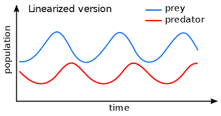
数学代写|数值方法作业代写numerical methods代考|Predator-Prey Models
ODEs can be used as simple models of population growth, for example, by assuming that the rate of reproduction of a population of size $P$ is proportional to the existing population and to the amount of available resources. The ODE is:
$$
\frac{d P}{d t}=r P\left(1-\frac{P}{K}\right), P(0)=P_{0}
$$
where $r$ is the growth rate and $K$ is the carrying capacity. The initial population is $P_{0}$. It is easy to check the following identities:
$$
P(t)=\frac{K P_{0} e^{r t}}{K+P_{0}\left(e^{r t}-1\right)} \text { and } \lim _{t \rightarrow \infty} P(t)=K .
$$
Transformation of this equation leads to the logistic ODE:
$$
\frac{d n}{d \tau}=n(1-n)
$$
where $n$ is the population in units of carrying capacity $(n=P / K)$ and $\tau$ measures time in units of $1 / r$.
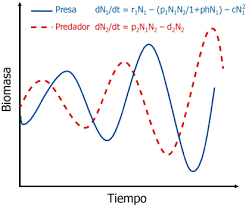
For systems, we can consider the predator-prey model in an environment consisting of foxes and rabbits:
$$
\begin{aligned}
&\frac{d r(t)}{d t}=-a r(t) f(t)+b r(t) \
&\frac{d f(t)}{d t}=-p f(t)+q f(t) r(t)
\end{aligned}
$$
where:
$$
\begin{aligned}
r(t) &=\text { number of rabbits at time } t \
f(t) &=\text { number of foxes at time } t \
b r(t) &=\text { birth rate of rabbits } \
-a r(t) f(t) &=\text { death rate of rabbits } \
b &=\text { unit birth rate of rabbits } \
-p f(t) &=\text { death rate of foxes } \
q f(t) r(t) &=\text { birth rate of foxes } \
q &=\text { unit birth rate of foxes. }
\end{aligned}
$$
The ODE system (3.14) is a model of a closed ecological environment in which foxes and rabbits are the only kinds of animals. Rabbits eat grass (of which there is a constant supply), procreate and are eaten by foxes. All foxes eat rabbits, procreate and die of geriatric diseases.
System (3.14) is sometimes called the Lotka-Volterra equations, which are an example of a more general Kolmogorov model to model the dynamics of ecological systems with predator-prey interactions, competition, disease and mutualism (Lotka (1956)).
数值方法代写
数学代写|数值方法作业代写numerical methods代考|An Example
我们采用一个简单的自治非线性标量 ODE 来展示如何计算 Picard 迭代:
是′=F(是)=是2,是(吨0)=一种
其解决方案由下式给出:
是(吨)=一种1−一种(吨−吨0)
我们现在计算这个 ODE 的 Picard 迭代 (3.4) 以确定吨ODE 有一个解决方案。为了方便,我们取一种=1,吨0=0. 一些简单的整合表明:
φ1(吨)=1 φ1(吨)=1+∫0吨F(φ0)d吨=1+吨 φ2(吨)=1+∫0吨F(φ1)d吨=1+吨+吨2+吨3/3 φ3(吨)=1+吨+吨2+吨3+2吨43+吨53+吨69+吨763
我们可以看到这个系列开始看起来像11−吨=∑j=0∞吨Ÿ. 我们知道这个系列是收敛的|吨|<1. 一个很好的练习是在最一般的情况下计算 Picard 迭代(即,一种≠1,吨0≠0) 并确定 ODE (3.6) 在何种情况下有解。在这种情况下,我们将 ODE 的解表示为一个系列,然后我们分析了这个系列,其中有很多收敛结果,例如根检验和比率检验。
数学代写|数值方法作业代写numerical methods代考|Riccati ODE
Riccati ODE 是以下形式的非线性 ODE:
是′=磷(X)+问(X)是+R(X)是2+ñ(X,是)
这个 ODE 有很多应用,例如利率模型(Duffie 和 Kan (1996))。在某些情况下,方程(3.10)的封闭形式的解是可能的,但在本书中,我们的重点是使用有限差分法对其进行近似。
我们现在讨论里卡蒂方程和零息债券定价之间的关系磷(吨,吨),这是一种在到期时提供一美元的合约吨. 根据定义,仿射期限结构模型假设磷(吨,吨)具有以下形式:
磷(吨,吨)=经验[一种(吨,吨)−乙(吨,吨)r(吨)]
让我们假设短期利率由以下随机微分方程 (SDE) 描述:
dr=μ(吨,r)d吨+σ(吨,r)d在吨
在哪里在吨是风险中性等价测度下的标准布朗运动,并且μ和σ被赋予功能。
Duffie 和 Kan 证明了磷(吨,吨)是指数仿射的当且仅当漂移μ和波动性σ有以下形式:
μ(吨,r)=一种(吨)r+b(吨),σ(吨,r)=C(吨)r+d(吨)
在哪里一种(吨),b(吨),C(吨)和d(吨)被赋予函数吨.
系数一种(吨,吨)和乙(吨,吨)在这种情况下,由以下常微分方程确定:
d乙d吨=C(吨)2乙(吨,吨)2−一种(吨)乙(吨,吨)−1,乙(吨,吨)=0
和:
d一种d吨=b(吨)乙(吨,吨)−d(吨)2乙(吨,吨)2,一种(吨,吨)=0
第一个方程(3.11)为乙(吨,吨)是 Riccati 方程,第二个方程 (3.12) 很容易通过积分从第一个方程求解。
数学代写|数值方法作业代写numerical methods代考|Predator-Prey Models
ODE 可以用作人口增长的简单模型,例如,通过假设磷与现有人口和可用资源量成正比。ODE 是:
d磷d吨=r磷(1−磷ķ),磷(0)=磷0
在哪里r是增长率和ķ是承载能力。初始人口为磷0. 很容易检查以下身份:
磷(吨)=ķ磷0和r吨ķ+磷0(和r吨−1) 和 林吨→∞磷(吨)=ķ.
该方程的变换导致逻辑 ODE:
dndτ=n(1−n)
在哪里n是以承载能力为单位的人口(n=磷/ķ)和τ以单位测量时间1/r.
对于系统,我们可以考虑由狐狸和兔子组成的环境中的捕食者-猎物模型:
dr(吨)d吨=−一种r(吨)F(吨)+br(吨) dF(吨)d吨=−pF(吨)+qF(吨)r(吨)
在哪里:
r(吨)= 一次兔子的数量 吨 F(吨)= 一次狐狸的数量 吨 br(吨)= 兔子的出生率 −一种r(吨)F(吨)= 兔子的死亡率 b= 兔单位出生率 −pF(吨)= 狐狸的死亡率 qF(吨)r(吨)= 狐狸出生率 q= 狐狸的单位出生率。
ODE系统(3.14)是一个封闭的生态环境模型,其中狐狸和兔子是唯一的动物。兔子吃草(其中有源源不断的供应),繁殖并被狐狸吃掉。所有的狐狸都吃兔子,生育并死于老年病。
系统 (3.14) 有时被称为 Lotka-Volterra 方程,它是更通用的 Kolmogorov 模型的一个例子,用于模拟具有捕食者-猎物相互作用、竞争、疾病和共生关系的生态系统动力学 (Lotka (1956))。

统计代写请认准statistics-lab™. statistics-lab™为您的留学生涯保驾护航。
金融工程代写
金融工程是使用数学技术来解决金融问题。金融工程使用计算机科学、统计学、经济学和应用数学领域的工具和知识来解决当前的金融问题,以及设计新的和创新的金融产品。
非参数统计代写
非参数统计指的是一种统计方法,其中不假设数据来自于由少数参数决定的规定模型;这种模型的例子包括正态分布模型和线性回归模型。
广义线性模型代考
广义线性模型(GLM)归属统计学领域,是一种应用灵活的线性回归模型。该模型允许因变量的偏差分布有除了正态分布之外的其它分布。
术语 广义线性模型(GLM)通常是指给定连续和/或分类预测因素的连续响应变量的常规线性回归模型。它包括多元线性回归,以及方差分析和方差分析(仅含固定效应)。
有限元方法代写
有限元方法(FEM)是一种流行的方法,用于数值解决工程和数学建模中出现的微分方程。典型的问题领域包括结构分析、传热、流体流动、质量运输和电磁势等传统领域。
有限元是一种通用的数值方法,用于解决两个或三个空间变量的偏微分方程(即一些边界值问题)。为了解决一个问题,有限元将一个大系统细分为更小、更简单的部分,称为有限元。这是通过在空间维度上的特定空间离散化来实现的,它是通过构建对象的网格来实现的:用于求解的数值域,它有有限数量的点。边界值问题的有限元方法表述最终导致一个代数方程组。该方法在域上对未知函数进行逼近。[1] 然后将模拟这些有限元的简单方程组合成一个更大的方程系统,以模拟整个问题。然后,有限元通过变化微积分使相关的误差函数最小化来逼近一个解决方案。
tatistics-lab作为专业的留学生服务机构,多年来已为美国、英国、加拿大、澳洲等留学热门地的学生提供专业的学术服务,包括但不限于Essay代写,Assignment代写,Dissertation代写,Report代写,小组作业代写,Proposal代写,Paper代写,Presentation代写,计算机作业代写,论文修改和润色,网课代做,exam代考等等。写作范围涵盖高中,本科,研究生等海外留学全阶段,辐射金融,经济学,会计学,审计学,管理学等全球99%专业科目。写作团队既有专业英语母语作者,也有海外名校硕博留学生,每位写作老师都拥有过硬的语言能力,专业的学科背景和学术写作经验。我们承诺100%原创,100%专业,100%准时,100%满意。
随机分析代写
随机微积分是数学的一个分支,对随机过程进行操作。它允许为随机过程的积分定义一个关于随机过程的一致的积分理论。这个领域是由日本数学家伊藤清在第二次世界大战期间创建并开始的。
时间序列分析代写
随机过程,是依赖于参数的一组随机变量的全体,参数通常是时间。 随机变量是随机现象的数量表现,其时间序列是一组按照时间发生先后顺序进行排列的数据点序列。通常一组时间序列的时间间隔为一恒定值(如1秒,5分钟,12小时,7天,1年),因此时间序列可以作为离散时间数据进行分析处理。研究时间序列数据的意义在于现实中,往往需要研究某个事物其随时间发展变化的规律。这就需要通过研究该事物过去发展的历史记录,以得到其自身发展的规律。
回归分析代写
多元回归分析渐进(Multiple Regression Analysis Asymptotics)属于计量经济学领域,主要是一种数学上的统计分析方法,可以分析复杂情况下各影响因素的数学关系,在自然科学、社会和经济学等多个领域内应用广泛。
MATLAB代写
MATLAB 是一种用于技术计算的高性能语言。它将计算、可视化和编程集成在一个易于使用的环境中,其中问题和解决方案以熟悉的数学符号表示。典型用途包括:数学和计算算法开发建模、仿真和原型制作数据分析、探索和可视化科学和工程图形应用程序开发,包括图形用户界面构建MATLAB 是一个交互式系统,其基本数据元素是一个不需要维度的数组。这使您可以解决许多技术计算问题,尤其是那些具有矩阵和向量公式的问题,而只需用 C 或 Fortran 等标量非交互式语言编写程序所需的时间的一小部分。MATLAB 名称代表矩阵实验室。MATLAB 最初的编写目的是提供对由 LINPACK 和 EISPACK 项目开发的矩阵软件的轻松访问,这两个项目共同代表了矩阵计算软件的最新技术。MATLAB 经过多年的发展,得到了许多用户的投入。在大学环境中,它是数学、工程和科学入门和高级课程的标准教学工具。在工业领域,MATLAB 是高效研究、开发和分析的首选工具。MATLAB 具有一系列称为工具箱的特定于应用程序的解决方案。对于大多数 MATLAB 用户来说非常重要,工具箱允许您学习和应用专业技术。工具箱是 MATLAB 函数(M 文件)的综合集合,可扩展 MATLAB 环境以解决特定类别的问题。可用工具箱的领域包括信号处理、控制系统、神经网络、模糊逻辑、小波、仿真等。