如果你也在 怎样代写计算复杂度理论Computational complexity theory这个学科遇到相关的难题,请随时右上角联系我们的24/7代写客服。
计算复杂度理论的重点是根据资源使用情况对计算问题进行分类,并将这些类别相互联系起来。计算问题是一项由计算机解决的任务。一个计算问题是可以通过机械地应用数学步骤来解决的,比如一个算法。
statistics-lab™ 为您的留学生涯保驾护航 在代写计算复杂度理论Computational complexity theory方面已经树立了自己的口碑, 保证靠谱, 高质且原创的统计Statistics代写服务。我们的专家在代写计算复杂度理论Computational complexity theory代写方面经验极为丰富,各种代写计算复杂度理论Computational complexity theory相关的作业也就用不着说。
我们提供的计算复杂度理论Computational complexity theory及其相关学科的代写,服务范围广, 其中包括但不限于:
- Statistical Inference 统计推断
- Statistical Computing 统计计算
- Advanced Probability Theory 高等概率论
- Advanced Mathematical Statistics 高等数理统计学
- (Generalized) Linear Models 广义线性模型
- Statistical Machine Learning 统计机器学习
- Longitudinal Data Analysis 纵向数据分析
- Foundations of Data Science 数据科学基础
数学代写|计算复杂度理论代写Computational complexity theory代考|Random Oracles
Consider the class $\mathcal{C}$ of all subsets of ${0,1}^{*}$ and define subclasses $\mathcal{A}=\left{A \in \mathcal{C}: P^{A}=N P^{A}\right}$ and $B=\left{B \in \mathcal{C}: P^{B} \neq N P^{B}\right}$. One of the approaches to study the relativized $P=$ ? $N P$ question is to compare the two subclasses $\mathcal{A}$ and $\mathcal{B}$ to see which one is larger. In this subsection, we give a brief introduction to this study based on the probability theory on the space $\mathcal{C}$.
To define the notion of probability on the space $\mathcal{C}$, it is most convenient to identify each element $X \in \mathcal{C}$ with its characteristic sequence $\alpha_{X}=\chi_{X}(\lambda) \chi_{X}(0) \chi_{X}(1) \chi_{X}(00) \ldots$ (i.e., the $k$ th bit of $\alpha_{X}$ is 1 if and only if the $k$ th string of ${0,1}^{*}$, under the lexicographic ordering, is in $\left.X\right)$ and treat $\mathcal{C}$ as the set of all infinite binary sequences or, equivalently, the Cartesian product ${0,1}^{\infty}$. We can define a topology on $\mathcal{C}$ by letting the set ${0,1}$ have the discrete topology and forming the product topology on $\mathcal{C}$. This is the well-known Cantor space. We now define the uniform probability measure $\mu$ on $\mathcal{C}$ as the product measure of the simple equiprobable measure on ${0,1}$, that is, $\mu{0}=\mu{1}=1 / 2$. In other words, for any integer $n \geq 1$, the $n$th bit of a random sequence $\alpha \in \mathcal{C}$ has the equal probability to be 0 or 1 . If we identify each real number in $[0,1]$ with its binary expansion, then this measure $\mu$ is the Lebesgue measure on $[0,1] . .^{5}$
For any $u \in{0,1}^{}$, let $\Gamma_{u}$ be the set of all infinite binary sequences that begin with $u$, that is, $\Gamma_{u}^{u}=\left{u \beta: \beta \in{0,1}^{\infty}\right}$. Each set $\Gamma_{u}$ is called a cylinder. All cylinders $\Gamma_{u}, u \in{0,1}^{}$, together form a basis of open neighborhoods of the space $\mathcal{C}$ (under the product topology). It is clear that $\mu\left(\Gamma_{u}\right)=2^{-|u|}$ for all $u \in{0,1}^{}$. The smallest $\sigma$-field containing all $\Gamma_{u}$, for all $u \in{0,1}^{}$, is called the Borel field. ${ }^{6}$ Each set in the Borel field, called a Borel set, is measurable.
The question of which of the two subclasses $\mathcal{A}$ and $B$ is larger can be formulated, in this setting, as to whether $\mu(\mathcal{A})$ is greater than $\mu(\mathcal{B})$. In the following, we show that $\mu(\mathcal{A})=0$.
An important idea behind the proof is Kolmogorov’s zero-one law of tail events, which implies that if an oracle class is insensitive to a finite number of bit changes, then its probability is either zero or one. This property holds for the classes $\mathcal{A}$ and $B$ as well as most other interesting oracle classes.
数学代写|计算复杂度理论代写Computational complexity theory代考|Structure of Relativized NP
Although the meaning of relativized collapsing and relativized separation results is still not clear, many relativized results have been proven. These results show a variety of possible relations between the well-known complexity classes. In this section, we demonstrate some of these relativized results on complexity classes within $N P$ to show what the possible relations are between $P, N P, N P \cap \operatorname{co} N P$, and $U P$. The relativized results on the classes beyond the class $N P$, that is, those on $N P, P H$, and $P S P A C E$, will be discussed in later chapters.
The proofs of the following results are all done by the stageconstruction diagonalization. The proofs sometimes need to satisfy simultaneously two or more potentially conflicting requirements that make the proofs more involved.
Theorem 4.20 (a) $(\exists A) P^{A} \neq N P^{A} \cap \operatorname{coN} P^{A} \neq N P^{A}$.
(b) $(\exists B) P^{B} \neq N P^{B}=\cos P^{B}$.
(c) $(\exists C) P^{C}=N P^{C} \cap \operatorname{coN} P^{C} \neq N P^{C}$.
Proof. (a): This can be done by a standard diagonalization proof. We leave it as an exercise (Exercise 4.16(a)).
(b): Let $\left{M_{i}\right}$ be an effective enumeration of all polynomial-time oracle DTMs and $\left{N_{i}\right}$ an effective enumeration of all polynomial-time oracle NTMs. For any set $B$, let $K_{B}=\left{\left\langle i, x, 0^{j}\right\rangle: N_{i}^{B}\right.$ accepts $x$ in $j$ moves $}$. Then, by the relativized proof of Theorem $2.11, K_{B}$ is $\leq_{m}^{P}$-complete for the class $N P^{B}$. Let $L_{B}=\left{0^{n}:(\exists x)|x|=n, x \in B\right}$. Then, it is clear that $L_{B} \in N P^{B}$. We are going to construct a set $B$ to satisfy the following requirements:
$R_{0, t}$ : for each $x$ of length $t, x \notin K_{B} \Longleftrightarrow(\exists y,|y|=t) x y \in B$, $R_{1, i}:(\exists n) 0^{n} \in L_{B} \Longleftrightarrow M_{i}^{A}$ does not accept $0^{n} .$
Note that if requirements $R_{0, t}$ are satisfied for all $t \geq 1$, then $\overline{K_{B}} \in N P^{B}$ and, hence, $N P^{B}=\operatorname{coN} N P^{B}$, and if requirements $R_{1, i}$ are satisfied for all $i \geq 1$, then $L_{B} \notin P^{B}$ and, hence, $P^{B} \neq N P^{B}$.
We construct set $B$ by a stage construction. At each stage $n$, we will construct finite sets $B_{n}$ and $B_{n}^{\prime}$ such that $B_{n-1} \subseteq B_{n}, B_{n-1}^{\prime} \subseteq B_{n}^{\prime}$, and $B_{n} \cap$ $B_{n}^{\prime}=\emptyset$ for all $n \geq 1$. Set $B$ is define as the union of all $B_{n}, n \geq 0$.
The requirement $R_{0, t}, t \geq 1$, is to be satisfied by direct diagonalization at stage $2 t$. The requirements $R_{1, i}, i \geq 1$, are to be satisfied by a delayed diagonalization in the odd stages. We always try to satisfy the requirement $R_{1, i}$ with the least $i$ such that $R_{1, i}$ is not yet satisfied. We cancel an integer $i$ when $R_{1, i}$ is satisfied. Before stage 1 , we assume that $B_{0}=B_{0}^{\prime}=\emptyset$ and that none of integers $i$ is cancelled.
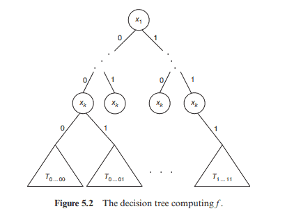
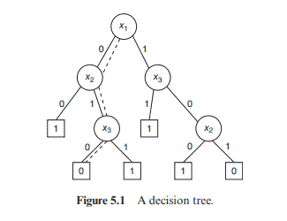
数学代写|计算复杂度理论代写Computational complexity theory代考|Graphs and Decision Trees
We first review the notion of graphs and the Boolean function representations of graphs. ${ }^{1}$ A graph is an ordered pair of disjoint sets $(V, E)$ such that $E$ is a set of pairs of elements in $V$ and $V \neq \emptyset$. The elements in the set $V$ are called vertices and the elements in the set $E$ are called edges. Two vertices are adjacent if there is an edge between them. Two graphs are isomorphic if there exists a one-to-one correspondence between their vertex sets that preserves adjacency.
A path is an alternating sequence of distinct vertices and edges starting and ending with vertices such that every vertex is an end point of its neighboring edges. The length of a path is the number of edges appearing in the path. A graph is connected if every pair of vertices are joined by a path.
Let $V={1, \ldots, n}$ be the vertex set of a graph $G=(V, E)$. Then its adjacency matrix $\left[x_{i j}\right]$ is defined by
$$
x_{i j}= \begin{cases}1 & \text { if }{i, j} \in E, \ 0 & \text { otherwise. }\end{cases}
$$
Note that $x_{i j}=x_{j i}$ and $x_{i i}=0$. So, the graph $G$ can be determined by $n(n-$ 1)/ 2 independent variables $x_{i j}, 1 \leq i<j \leq n$. For any property $\mathcal{P}$ of graphs with $n$ vertices, we define a Boolean function $f_{p}$ over $n(n-1) / 2$ variables $x_{i j}, 1 \leq i<j \leq n$, as follows:
$$
f_{p}\left(x_{12}, \ldots, x_{n-1, n}\right)= \begin{cases}1 & \begin{array}{l}
\text { if the graph } G \text { represented by }\left[x_{i, j}\right] \text { has } \
\text { the property } \mathcal{P}
\end{array} \
0 & \text { otherwise. }\end{cases}
$$
Then $\mathcal{P}$ can be determined by $f_{p}$. For example, the property of connectivity corresponds to the Boolean functions $f_{\text {con }}$ of $n(n-1) / 2$ variables such that $f_{c o n}\left(x_{12}, \ldots, x_{n-1, n}\right)=1$ if and only if the graph $G$ represented by $\left[x_{i j}\right]$ is connected.
Not every Boolean function of $n(n-1) / 2$ variables represents a graph property because a graph property should be invariant under graph isomorphism. A Boolean function $f$ of $n(n-1) / 2$ variables is called a graph property if for every permutation $\sigma$ on the vertex set ${1, \ldots, n}$,
$$
f\left(x_{12}, \ldots, x_{n-1, n}\right)=f\left(x_{\sigma(1) \sigma(2)}, \ldots, x_{\sigma(n-1) \sigma(n)}\right) \text {. }
$$
计算复杂度理论代考
数学代写|计算复杂度理论代写Computational complexity theory代考|Random Oracles
考虑班级C的所有子集0,1∗并定义子类\mathcal{A}=\left{A \in \mathcal{C}: P^{A}=N P^{A}\right}\mathcal{A}=\left{A \in \mathcal{C}: P^{A}=N P^{A}\right}和B=\left{B \in \mathcal{C}: P^{B} \neq N P^{B}\right}B=\left{B \in \mathcal{C}: P^{B} \neq N P^{B}\right}. 研究相对化的方法之一磷= ? ñ磷问题是比较两个子类一个和乙看看哪个更大。在本小节中,我们将简要介绍基于空间概率论的这项研究C.
在空间上定义概率的概念C, 最方便识别每个元素X∈C以其特征序列一个X=χX(λ)χX(0)χX(1)χX(00)…(即,ķ第一点一个X为 1 当且仅当ķ第一个字符串0,1∗,在词典排序下,在X)并对待C作为所有无限二进制序列的集合,或者等价地,笛卡尔积0,1∞. 我们可以定义一个拓扑C通过让集合0,1具有离散拓扑并形成产品拓扑C. 这就是著名的康托尔空间。我们现在定义统一概率测度μ上C作为简单等概率测度的乘积测度0,1, 那是,μ0=μ1=1/2. 换句话说,对于任何整数n≥1, 这n随机序列的第 th 位一个∈C为 0 或 1 的概率相等。如果我们识别出每个实数[0,1]用它的二进制展开,那么这个度量μ是 Lebesgue 测度[0,1]..5
对于任何在∈0,1, 让Γ在是所有以在, 那是,\Gamma_{u}^{u}=\left{u \beta: \beta \in{0,1}^{\infty}\right}\Gamma_{u}^{u}=\left{u \beta: \beta \in{0,1}^{\infty}\right}. 每套Γ在称为圆柱体。所有气缸Γ在,在∈0,1,共同构成空间开放邻域的基础C(在产品拓扑下)。很清楚μ(Γ在)=2−|在|对所有人在∈0,1. 最小的σ- 包含所有内容的字段Γ在, 对所有人在∈0,1,称为 Borel 场。6Borel 域中的每个集合(称为 Borel 集)都是可测量的。
两个子类中的哪一个的问题一个和乙在这种情况下,可以表述为更大,至于是否μ(一个)大于μ(乙). 在下文中,我们展示了μ(一个)=0.
证明背后的一个重要思想是 Kolmogorov 的尾事件零一定律,这意味着如果一个预言机类对有限数量的比特变化不敏感,那么它的概率为零或一。该属性适用于类一个和乙以及大多数其他有趣的 Oracle 类。
数学代写|计算复杂度理论代写Computational complexity theory代考|Structure of Relativized NP
虽然相对化坍缩和相对化分离结果的意义尚不明确,但许多相对化结果已被证明。这些结果显示了众所周知的复杂性类别之间的各种可能的关系。在本节中,我们展示了其中一些关于复杂性类的相对化结果ñ磷显示之间可能的关系磷,ñ磷,ñ磷∩合作ñ磷, 和在磷. 类外类的相对化结果ñ磷,也就是那些在ñ磷,磷H, 和磷小号磷一个C和, 将在后面的章节中讨论。
以下结果的证明都是通过stageconstruction对角化来完成的。证明有时需要同时满足两个或多个可能相互冲突的要求,这使得证明更加复杂。
定理 4.20 (a)(∃一个)磷一个≠ñ磷一个∩和磷一个≠ñ磷一个.
(二)(∃乙)磷乙≠ñ磷乙=因磷乙.
(C)(∃C)磷C=ñ磷C∩和磷C≠ñ磷C.
证明。(a):这可以通过标准的对角化证明来完成。我们把它作为一个练习(练习 4.16(a))。
(b): 让\left{M_{i}\right}\left{M_{i}\right}是所有多项式时间预言机 DTM 的有效枚举,并且\left{N_{i}\right}\left{N_{i}\right}所有多项式时间预言机 NTM 的有效枚举。对于任何集合乙, 让K_{B}=\left{\left\langle i, x, 0^{j}\right\rangle: N_{i}^{B}\right.$ 接受 $x$ 在 $j$ 移动 $}K_{B}=\left{\left\langle i, x, 0^{j}\right\rangle: N_{i}^{B}\right.$ 接受 $x$ 在 $j$ 移动 $}. 然后,由定理的相对化证明2.11,ķ乙是≤米磷- 完成课程ñ磷乙. 让L_{B}=\left{0^{n}:(\exists x)|x|=n, x \in B\right}L_{B}=\left{0^{n}:(\exists x)|x|=n, x \in B\right}. 那么,很明显大号乙∈ñ磷乙. 我们将构建一个集合乙满足以下要求:
R0,吨: 对于每个X长度吨,X∉ķ乙⟺(∃是,|是|=吨)X是∈乙, R1,一世:(∃n)0n∈大号乙⟺米一世一个不接受0n.
请注意,如果要求R0,吨对所有人都满意吨≥1, 然后ķ乙¯∈ñ磷乙因此,ñ磷乙=和ñ磷乙, 如果要求R1,一世对所有人都满意一世≥1, 然后大号乙∉磷乙因此,磷乙≠ñ磷乙.
我们构造集合乙通过阶段性建设。在每个阶段n,我们将构造有限集乙n和乙n′这样乙n−1⊆乙n,乙n−1′⊆乙n′, 和乙n∩ 乙n′=∅对所有人n≥1. 放乙被定义为所有的联合乙n,n≥0.
要求R0,吨,吨≥1, 在阶段通过直接对角化来满足2吨. 要求R1,一世,一世≥1, 将通过奇数阶段的延迟对角化来满足。我们总是努力满足要求R1,一世用最少的一世这样R1,一世还不满意。我们取消一个整数一世什么时候R1,一世很满意。在第一阶段之前,我们假设乙0=乙0′=∅并且没有整数一世取消。
数学代写|计算复杂度理论代写Computational complexity theory代考|Graphs and Decision Trees
我们首先回顾图的概念和图的布尔函数表示。1图是一组有序的不相交集(在,和)这样和是一组元素对在和在≠∅. 集合中的元素在被称为顶点和集合中的元素和称为边。如果两个顶点之间有边,则两个顶点相邻。如果两个图的顶点集之间存在保持邻接的一一对应关系,则两个图是同构的。
路径是不同顶点和边的交替序列,以顶点开始和结束,使得每个顶点都是其相邻边的端点。路径的长度是路径中出现的边数。如果每对顶点都通过路径连接,则图是连通的。
让在=1,…,n是一个图的顶点集G=(在,和). 那么它的邻接矩阵[X一世j]定义为
X一世j={1 如果 一世,j∈和, 0 否则。
注意X一世j=Xj一世和X一世一世=0. 所以,图G可由下式确定n(n−1)/ 2个自变量X一世j,1≤一世<j≤n. 对于任何财产磷图表与n顶点,我们定义一个布尔函数Fp超过n(n−1)/2变量X一世j,1≤一世<j≤n, 如下:
Fp(X12,…,Xn−1,n)={1 如果图表 G 代表为 [X一世,j] 有 财产 磷 0 否则。
然后磷可由下式确定Fp. 例如,连通性的属性对应于布尔函数F和 的n(n−1)/2变量使得FC○n(X12,…,Xn−1,n)=1当且仅当图形G代表为[X一世j]已连接。
不是每个布尔函数n(n−1)/2variables 表示图属性,因为图属性在图同构下应该是不变的。布尔函数F的n(n−1)/2如果对于每个排列,变量被称为图形属性σ在顶点集上1,…,n,
F(X12,…,Xn−1,n)=F(Xσ(1)σ(2),…,Xσ(n−1)σ(n)).

统计代写请认准statistics-lab™. statistics-lab™为您的留学生涯保驾护航。
金融工程代写
金融工程是使用数学技术来解决金融问题。金融工程使用计算机科学、统计学、经济学和应用数学领域的工具和知识来解决当前的金融问题,以及设计新的和创新的金融产品。
非参数统计代写
非参数统计指的是一种统计方法,其中不假设数据来自于由少数参数决定的规定模型;这种模型的例子包括正态分布模型和线性回归模型。
广义线性模型代考
广义线性模型(GLM)归属统计学领域,是一种应用灵活的线性回归模型。该模型允许因变量的偏差分布有除了正态分布之外的其它分布。
术语 广义线性模型(GLM)通常是指给定连续和/或分类预测因素的连续响应变量的常规线性回归模型。它包括多元线性回归,以及方差分析和方差分析(仅含固定效应)。
有限元方法代写
有限元方法(FEM)是一种流行的方法,用于数值解决工程和数学建模中出现的微分方程。典型的问题领域包括结构分析、传热、流体流动、质量运输和电磁势等传统领域。
有限元是一种通用的数值方法,用于解决两个或三个空间变量的偏微分方程(即一些边界值问题)。为了解决一个问题,有限元将一个大系统细分为更小、更简单的部分,称为有限元。这是通过在空间维度上的特定空间离散化来实现的,它是通过构建对象的网格来实现的:用于求解的数值域,它有有限数量的点。边界值问题的有限元方法表述最终导致一个代数方程组。该方法在域上对未知函数进行逼近。[1] 然后将模拟这些有限元的简单方程组合成一个更大的方程系统,以模拟整个问题。然后,有限元通过变化微积分使相关的误差函数最小化来逼近一个解决方案。
tatistics-lab作为专业的留学生服务机构,多年来已为美国、英国、加拿大、澳洲等留学热门地的学生提供专业的学术服务,包括但不限于Essay代写,Assignment代写,Dissertation代写,Report代写,小组作业代写,Proposal代写,Paper代写,Presentation代写,计算机作业代写,论文修改和润色,网课代做,exam代考等等。写作范围涵盖高中,本科,研究生等海外留学全阶段,辐射金融,经济学,会计学,审计学,管理学等全球99%专业科目。写作团队既有专业英语母语作者,也有海外名校硕博留学生,每位写作老师都拥有过硬的语言能力,专业的学科背景和学术写作经验。我们承诺100%原创,100%专业,100%准时,100%满意。
随机分析代写
随机微积分是数学的一个分支,对随机过程进行操作。它允许为随机过程的积分定义一个关于随机过程的一致的积分理论。这个领域是由日本数学家伊藤清在第二次世界大战期间创建并开始的。
时间序列分析代写
随机过程,是依赖于参数的一组随机变量的全体,参数通常是时间。 随机变量是随机现象的数量表现,其时间序列是一组按照时间发生先后顺序进行排列的数据点序列。通常一组时间序列的时间间隔为一恒定值(如1秒,5分钟,12小时,7天,1年),因此时间序列可以作为离散时间数据进行分析处理。研究时间序列数据的意义在于现实中,往往需要研究某个事物其随时间发展变化的规律。这就需要通过研究该事物过去发展的历史记录,以得到其自身发展的规律。
回归分析代写
多元回归分析渐进(Multiple Regression Analysis Asymptotics)属于计量经济学领域,主要是一种数学上的统计分析方法,可以分析复杂情况下各影响因素的数学关系,在自然科学、社会和经济学等多个领域内应用广泛。
MATLAB代写
MATLAB 是一种用于技术计算的高性能语言。它将计算、可视化和编程集成在一个易于使用的环境中,其中问题和解决方案以熟悉的数学符号表示。典型用途包括:数学和计算算法开发建模、仿真和原型制作数据分析、探索和可视化科学和工程图形应用程序开发,包括图形用户界面构建MATLAB 是一个交互式系统,其基本数据元素是一个不需要维度的数组。这使您可以解决许多技术计算问题,尤其是那些具有矩阵和向量公式的问题,而只需用 C 或 Fortran 等标量非交互式语言编写程序所需的时间的一小部分。MATLAB 名称代表矩阵实验室。MATLAB 最初的编写目的是提供对由 LINPACK 和 EISPACK 项目开发的矩阵软件的轻松访问,这两个项目共同代表了矩阵计算软件的最新技术。MATLAB 经过多年的发展,得到了许多用户的投入。在大学环境中,它是数学、工程和科学入门和高级课程的标准教学工具。在工业领域,MATLAB 是高效研究、开发和分析的首选工具。MATLAB 具有一系列称为工具箱的特定于应用程序的解决方案。对于大多数 MATLAB 用户来说非常重要,工具箱允许您学习和应用专业技术。工具箱是 MATLAB 函数(M 文件)的综合集合,可扩展 MATLAB 环境以解决特定类别的问题。可用工具箱的领域包括信号处理、控制系统、神经网络、模糊逻辑、小波、仿真等。