数学代写|计量经济学原理代写Principles of Econometrics代考|A Failure of the Exogeneity Assumption

statistics-lab™ 为您的留学生涯保驾护航在代写计量经济学Principles of Econometrics方面已经树立了自己的口碑, 保证靠谱, 高质且原创的统计Statistics代写服务。我们的专家在代写计量经济学Principles of Econometrics代写方面经验极为丰富，各种代写计量经济学Principles of Econometrics相关的作业也就用不着说。

我们提供的计量经济学Principles of Econometrics及其相关学科的代写，服务范围广, 其中包括但不限于:

Statistical Inference 统计推断
Statistical Computing 统计计算
Advanced Probability Theory 高等概率论
Advanced Mathematical Statistics 高等数理统计学
(Generalized) Linear Models 广义线性模型
Statistical Machine Learning 统计机器学习
Longitudinal Data Analysis 纵向数据分析
Foundations of Data Science 数据科学基础

数学代写|计量经济学原理代写Principles of Econometrics代考|A Failure of the Exogeneity Assumption

数学代写|计量经济学原理代写Principles of Econometrics代考|The Regression Function

The importance of the strict exogeneity assumption is the following. If the strict exogeneity assumption $E\left(e_{i} \mid x_{i}\right)=0$ is true, then the conditional expectation of $y_{i}$ given $x_{i}$ is
$$
E\left(y_{i} \mid x_{i}\right)=\beta_{1}+\beta_{2} x_{i}+E\left(e_{i} \mid x_{i}\right)=\beta_{1}+\beta_{2} x_{i}, \quad i=1, \ldots, N
$$
The conditional expectation $E\left(y_{i} \mid x_{i}\right)=\beta_{1}+\beta_{2} x_{i}$ in (2.2) is called the regression function, or population regression function. It says that in the population the average value of the dependent variable for the $i$ th observation, conditional on $x_{i}$, is given by $\beta_{1}+\beta_{2} x_{i}$. It also says that given a change in $x, \Delta x$, the resulting change in $E\left(y_{i} \mid x_{i}\right)$ is $\beta_{2} \Delta x$ holding all else constant, in the sense that given $x_{i}$ the average of the random errors is zero, and any change in $x$ is not correlated with any corresponding change in the random error $e$. In this case, we can say that a change in $x$ leads to, or causes, a change in the expected (population average) value of $y$ given $x_{i}, E\left(y_{i} \mid x_{i}\right)$.

The regression function in (2.2) is shown in Figure 2.2, with $y$-intercept $\beta_{1}=E\left(y_{i} \mid x_{i}=0\right)$ and slope
$$
\beta_{2}=\frac{\Delta E\left(y_{i} \mid x_{i}\right)}{\Delta x_{i}}=\frac{d E\left(y_{i} \mid x_{i}\right)}{d x_{i}}
$$
where $\Delta$ denotes “change in” and $d E(y \mid x) / d x$ denotes the “derivative” of $E(y \mid x)$ with respect to $x$. We will not use derivatives to any great extent in this book, and if you are not too familiar with the concept you can think of ” $d “$ ” as a stylized version of $\Delta$ and go on. See Appendix A.3 for a discussion of derivatives.

数学代写|计量经济学原理代写Principles of Econometrics代考|Strict Exogeneity in the Household Food Expenditure Model

Another important consequence of the assumption of strict exogeneity is that it allows us to think of the econometric model as decomposing the dependent variable into two components: one that yaries systematically as the values of the independent variable change and another that is random “noise.” That is, the econometric model $y_{i}=\beta_{1}+\beta_{2} x_{i}+e_{i}$ can be broken into two parts: $E\left(y_{i} \mid x_{i}\right)=\beta_{1}+\beta_{2} x_{i}$ and the random error, $e_{i}$. Thus
$$
y_{i}=\beta_{1}+\beta_{2} x_{i}+e_{i}=E\left(y_{i} \mid x_{i}\right)+e_{i}
$$
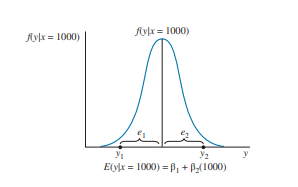
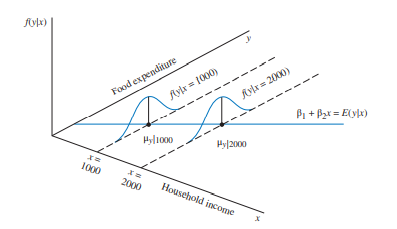
The values of the dependent variable $y_{i}$ vary systematically due to variation in the conditional mean $E\left(y_{i} \mid x_{i}\right)=\beta_{1}+\beta_{2} x_{i}$, as the value of the explanatory variable changes, and the values of the dependent variable $y_{i}$ vary randomly due to $e_{i}$. The conditional $p d f \mathrm{~s}$ of $e$ and $y$ are identical except for their location, as shown in Figure 2.3. Two values of food expenditure $y_{1}$ and $y_{2}$ for households with $x=\$ 1000$ of weekly income are shown in Figure $2.4$ relative to their conditional mean. There will be variation in household expenditures on food from one household to another because of variations in tastes and preferences, and everything else. Some will spend more than the average value for households with the same income, and some will spend less. If we knew $\beta_{1}$ and $\beta_{2}$, then we could compute the conditional mean expenditure $E\left(y_{t} \mid x=1000\right)=\beta_{1}+\beta_{2}(1000)$ and also the value of the random errors $e_{1}$ and $e_{2}$. We never know $\beta_{1}$ and $\beta_{2}$ so we can never compute $e_{1}$ and $e_{2}$. What we are assuming, however, is that at each level of income $x$ the average value of all that is represented by the random error is zero.

数学代写|计量经济学原理代写Principles of Econometrics代考|Error Normality

In the discussion surrounding Figure 2.1, we explicitly made the assumption that food expenditures, given income, were normally distributed. In Figures $2.3-2.5$, we implicitly made the assumption of conditionally normally distributed errors and dependent variable by drawing classically bell-shaped curves. It is not at all necessary for the random errors to be conditionally normal in order for regression analysis to “work.” However, as you will discover in Chapter 3 , when samples are small, it is advantageous for statistical inferences that the random errors, and dependent variable $y$, given each $x$-value, are normally distributed. The normal distribution has a long and interesting history, ${ }^{3}$ as a little Internet searching will reveal. One argument for assuming regression errors are normally distributed is that they represent a collection of many different factors. The Central Limit Theorem, see Appendix C.3.4, says roughly that collections of many random factors tend toward having a normal distribution. In the context of the food expenditure model, if we consider that the random errors reflect tastes and preferences, it is entirely plausible that the random errors at each income level are normally distributed. When the assumption of conditionally normal errors is made, we write $e_{i} \mid x_{i} \sim N\left(0, \sigma^{2}\right)$ and also then $y_{i} \mid x_{i} \sim N\left(\beta_{1}+\beta_{2} x_{i}, \sigma^{2}\right)$. It is a very strong assumption when it is made, and as mentioned it is not strictly speaking necessary, so we call it an optional assumption.

In a regression analysis, one of the objectives is to estimate $\beta_{2}=\Delta E\left(y_{i} \mid x_{i}\right) / \Delta x_{i}$. If we are to hope that a sample of data can be used to estimate the effects of changes in $x$, then we must observe some different values of the explanatory variable $x$ in the sample. Intuitively, if we collect data only on households with income $\$ 1000$, we will not be able to measure the effect of changing income on the average value of food expenditure. Recall from elementary geometry that “it takes two points to determine a line.” The minimum number of $x$-values in a sample of data that will allow us to proceed is two. You will find out in Section 2.4.4 that in fact the more different values of $x$, and the more variation they exhibit, the better our regression analysis will be.

计量经济学代考

数学代写|计量经济学原理代写Principles of Econometrics代考|The Regression Function

严格外生性假设的重要性如下。如果严格的外生假设和(和一世∣X一世)=0为真，则条件期望为是一世给定X一世是

和(是一世∣X一世)=b1+b2X一世+和(和一世∣X一世)=b1+b2X一世,一世=1,…,ñ
有条件的期望和(是一世∣X一世)=b1+b2X一世（2.2）中的称为回归函数或总体回归函数。它说在总体中，因变量的平均值一世第一次观察，条件是X一世，是（谁）给的b1+b2X一世. 它还说，鉴于X,ΔX，由此产生的变化和(是一世∣X一世)是b2ΔX在给定的意义上，保持所有其他不变X一世随机误差的平均值为零，任何变化X与随机误差的任何相应变化无关和. 在这种情况下，我们可以说改变X导致或导致预期（总体平均）值的变化是给定X一世,和(是一世∣X一世).

（2.2）中的回归函数如图 2.2 所示，其中是-截距b1=和(是一世∣X一世=0)和坡度

b2=Δ和(是一世∣X一世)ΔX一世=d和(是一世∣X一世)dX一世
在哪里Δ表示“变化”和d和(是∣X)/dX表示的“衍生物”和(是∣X)关于X. 我们不会在本书中大量使用衍生品，如果你对这个概念不太熟悉，你可以想到”d“”作为一个程式化的版本Δ继续。有关衍生产品的讨论，请参见附录 A.3。

数学代写|计量经济学原理代写Principles of Econometrics代考|Strict Exogeneity in the Household Food Expenditure Model

严格外生性假设的另一个重要结果是，它允许我们将计量经济模型视为将因变量分解为两个部分：一个随着自变量值的变化而系统地变化，另一个是随机的“噪声”。也就是说，计量经济学模型是一世=b1+b2X一世+和一世可以分为两部分：和(是一世∣X一世)=b1+b2X一世和随机误差，和一世. 因此

是一世=b1+b2X一世+和一世=和(是一世∣X一世)+和一世
因变量的值是一世由于条件均值的变化而系统地变化和(是一世∣X一世)=b1+b2X一世，随着解释变量的值变化，因变量的值变化是一世由于随机变化和一世. 有条件的pdF s的和和是除了它们的位置之外，它们是相同的，如图 2.3 所示。食品支出的两种价值是1和是2对于有家庭X=$1000每周收入如图2.4相对于他们的条件均值。由于口味和偏好以及其他因素的不同，每个家庭的家庭食品支出都会有所不同。有些人的支出会超过收入相同的家庭的平均水平，有些人的支出会更少。如果我们知道b1和b2，那么我们可以计算条件平均支出和(是吨∣X=1000)=b1+b2(1000)以及随机误差的值和1和和2. 我们不知道b1和b2所以我们永远无法计算和1和和2. 然而，我们假设的是，在每个收入水平X所有由随机误差表示的平均值为零。

数学代写|计量经济学原理代写Principles of Econometrics代考|Error Normality

在围绕图 2.1 的讨论中，我们明确假设在给定收入的情况下，食品支出是正态分布的。在数字2.3−2.5，我们通过绘制经典的钟形曲线隐含地假设条件正态分布的误差和因变量。为了使回归分析“起作用”，随机误差完全不需要条件正态。但是，正如您将在第 3 章中发现的那样，当样本较小时，随机误差和因变量对统计推断是有利的是，给定每个X-值，正态分布。正态分布有着悠久而有趣的历史，3正如一点互联网搜索所揭示的那样。假设回归误差是正态分布的一个论据是它们代表了许多不同因素的集合。中心极限定理，见附录 C.3.4，粗略地说，许多随机因素的集合倾向于具有正态分布。在食品支出模型的背景下，如果我们认为随机误差反映了口味和偏好，那么每个收入水平的随机误差都是正态分布的，这是完全合理的。当假设条件正态错误时，我们写和一世∣X一世∼ñ(0,σ2)然后也是是一世∣X一世∼ñ(b1+b2X一世,σ2). 这是一个非常强的假设，如前所述，严格来说它不是必需的，所以我们称之为可选假设。

在回归分析中，目标之一是估计b2=Δ和(是一世∣X一世)/ΔX一世. 如果我们希望可以使用数据样本来估计变化的影响X，那么我们必须观察解释变量的一些不同的值X在样本中。直观地说，如果我们只收集有收入家庭的数据$1000，我们将无法衡量收入变化对食品支出平均值的影响。回想一下初等几何“确定一条线需要两个点”。最少数量X允许我们继续进行的数据样本中的值是两个。您将在第 2.4.4 节中发现，实际上更多不同的值X，并且它们表现出的变化越多，我们的回归分析就越好。

数学代写|计量经济学原理代写Principles of Econometrics代考请认准statistics-lab™

统计代写请认准statistics-lab™. statistics-lab™为您的留学生涯保驾护航。

金融工程代写

金融工程是使用数学技术来解决金融问题。金融工程使用计算机科学、统计学、经济学和应用数学领域的工具和知识来解决当前的金融问题，以及设计新的和创新的金融产品。

非参数统计代写

非参数统计指的是一种统计方法，其中不假设数据来自于由少数参数决定的规定模型；这种模型的例子包括正态分布模型和线性回归模型。

广义线性模型代考

广义线性模型（GLM）归属统计学领域，是一种应用灵活的线性回归模型。该模型允许因变量的偏差分布有除了正态分布之外的其它分布。

术语广义线性模型（GLM）通常是指给定连续和/或分类预测因素的连续响应变量的常规线性回归模型。它包括多元线性回归，以及方差分析和方差分析（仅含固定效应）。

有限元方法代写

有限元方法（FEM）是一种流行的方法，用于数值解决工程和数学建模中出现的微分方程。典型的问题领域包括结构分析、传热、流体流动、质量运输和电磁势等传统领域。

有限元是一种通用的数值方法，用于解决两个或三个空间变量的偏微分方程（即一些边界值问题）。为了解决一个问题，有限元将一个大系统细分为更小、更简单的部分，称为有限元。这是通过在空间维度上的特定空间离散化来实现的，它是通过构建对象的网格来实现的：用于求解的数值域，它有有限数量的点。边界值问题的有限元方法表述最终导致一个代数方程组。该方法在域上对未知函数进行逼近。[1] 然后将模拟这些有限元的简单方程组合成一个更大的方程系统，以模拟整个问题。然后，有限元通过变化微积分使相关的误差函数最小化来逼近一个解决方案。

tatistics-lab作为专业的留学生服务机构，多年来已为美国、英国、加拿大、澳洲等留学热门地的学生提供专业的学术服务，包括但不限于Essay代写，Assignment代写，Dissertation代写，Report代写，小组作业代写，Proposal代写，Paper代写，Presentation代写，计算机作业代写，论文修改和润色，网课代做，exam代考等等。写作范围涵盖高中，本科，研究生等海外留学全阶段，辐射金融，经济学，会计学，审计学，管理学等全球99%专业科目。写作团队既有专业英语母语作者，也有海外名校硕博留学生，每位写作老师都拥有过硬的语言能力，专业的学科背景和学术写作经验。我们承诺100%原创，100%专业，100%准时，100%满意。

随机分析代写

随机微积分是数学的一个分支，对随机过程进行操作。它允许为随机过程的积分定义一个关于随机过程的一致的积分理论。这个领域是由日本数学家伊藤清在第二次世界大战期间创建并开始的。

时间序列分析代写

随机过程，是依赖于参数的一组随机变量的全体，参数通常是时间。随机变量是随机现象的数量表现，其时间序列是一组按照时间发生先后顺序进行排列的数据点序列。通常一组时间序列的时间间隔为一恒定值（如1秒，5分钟，12小时，7天，1年），因此时间序列可以作为离散时间数据进行分析处理。研究时间序列数据的意义在于现实中，往往需要研究某个事物其随时间发展变化的规律。这就需要通过研究该事物过去发展的历史记录，以得到其自身发展的规律。

回归分析代写

多元回归分析渐进（Multiple Regression Analysis Asymptotics）属于计量经济学领域，主要是一种数学上的统计分析方法，可以分析复杂情况下各影响因素的数学关系，在自然科学、社会和经济学等多个领域内应用广泛。

MATLAB代写

MATLAB 是一种用于技术计算的高性能语言。它将计算、可视化和编程集成在一个易于使用的环境中，其中问题和解决方案以熟悉的数学符号表示。典型用途包括：数学和计算算法开发建模、仿真和原型制作数据分析、探索和可视化科学和工程图形应用程序开发，包括图形用户界面构建MATLAB 是一个交互式系统，其基本数据元素是一个不需要维度的数组。这使您可以解决许多技术计算问题，尤其是那些具有矩阵和向量公式的问题，而只需用 C 或 Fortran 等标量非交互式语言编写程序所需的时间的一小部分。MATLAB 名称代表矩阵实验室。MATLAB 最初的编写目的是提供对由 LINPACK 和 EISPACK 项目开发的矩阵软件的轻松访问，这两个项目共同代表了矩阵计算软件的最新技术。MATLAB 经过多年的发展，得到了许多用户的投入。在大学环境中，它是数学、工程和科学入门和高级课程的标准教学工具。在工业领域，MATLAB 是高效研究、开发和分析的首选工具。MATLAB 具有一系列称为工具箱的特定于应用程序的解决方案。对于大多数 MATLAB 用户来说非常重要，工具箱允许您学习和应用专业技术。工具箱是 MATLAB 函数（M 文件）的综合集合，可扩展 MATLAB 环境以解决特定类别的问题。可用工具箱的领域包括信号处理、控制系统、神经网络、模糊逻辑、小波、仿真等。

R语言代写	问卷设计与分析代写
PYTHON代写	回归分析与线性模型代写
MATLAB代写	方差分析与试验设计代写
STATA代写	机器学习/统计学习代写
SPSS代写	计量经济学代写
EVIEWS代写	时间序列分析代写
EXCEL代写	深度学习代写
SQL代写	各种数据建模与可视化代写