ECMT5001 - 统计代写答疑辅导

标签： ECMT5001

数学代写|计量经济学原理代写Principles of Econometrics代考|Estimating the Regression Parameters

Posted on 2022年6月1日2022年6月1日 by statistics-lab

如果你也在怎样代写计量经济学Principles of Econometrics这个学科遇到相关的难题，请随时右上角联系我们的24/7代写客服。

计量经济学是以数理经济学和数理统计学为方法论基础，对于经济问题试图对理论上的数量接近和经验（实证研究）上的数量接近这两者进行综合而产生的经济学分支。

statistics-lab™ 为您的留学生涯保驾护航在代写计量经济学Principles of Econometrics方面已经树立了自己的口碑, 保证靠谱, 高质且原创的统计Statistics代写服务。我们的专家在代写计量经济学Principles of Econometrics代写方面经验极为丰富，各种代写计量经济学Principles of Econometrics相关的作业也就用不着说。

我们提供的计量经济学Principles of Econometrics及其相关学科的代写，服务范围广, 其中包括但不限于:

Statistical Inference 统计推断
Statistical Computing 统计计算
Advanced Probability Theory 高等概率论
Advanced Mathematical Statistics 高等数理统计学
(Generalized) Linear Models 广义线性模型
Statistical Machine Learning 统计机器学习
Longitudinal Data Analysis 纵向数据分析
Foundations of Data Science 数据科学基础

数学代写|计量经济学原理代写Principles of Econometrics代考|Estimating the Regression Parameters

数学代写|计量经济学原理代写Principles of Econometrics代考|Food Expenditure Model Data

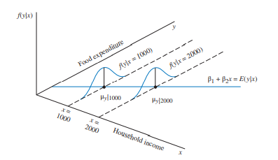
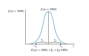
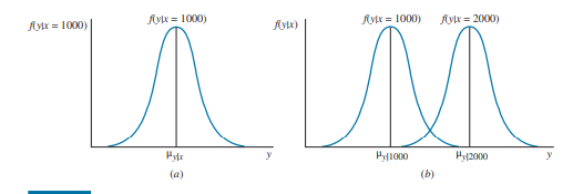
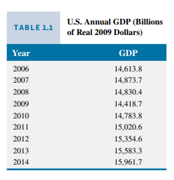
We assume that the expenditure data in Table $2.1$ satisfy the assumptions SR1-SR5. That is, we assume that the regression model $y_{i}=\beta_{1}+\beta_{2} x_{i}+e_{i}$ describes a population relationship and that the random error has conditional expected value zero. This implies that the conditional expected value of household food expenditure is a linear function of income. The conditional variance of $y$, which is the same as that of the random error $e$, is assumed constant, implying that we are equally uncertain about the relationship between $y$ and $x$ for all observations. Given $\mathbf{x}$ the values of $y$ for different households are assumed uncorrelated with each other.

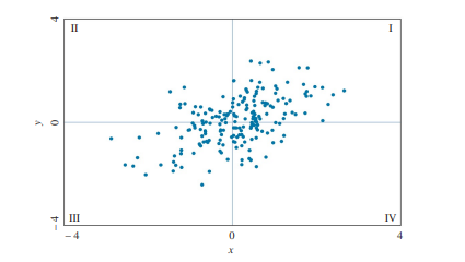
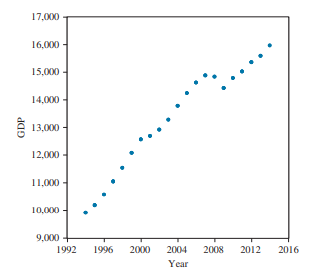
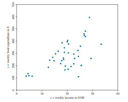
Given this theoretical model for explaining the sample observations on household food expenditure, the problem now is how to use the sample information in Table 2.1, specific values of $y_{i}$ and $x_{i}$, to estimate the unknown regression parameters $\beta_{1}$ and $\beta_{2}$. These parameters represent the unknown intercept and slope coefficients for the food expenditure-income relationship. If we represent the 40 data points as $\left(y_{i}, x_{i}\right), i=1, \ldots, N=40$, and plot them, we obtain the scatter diagram in Figure $2.6$.Our problem is to estimate the location of the mean expenditure line $E\left(y_{i} \mid \mathbf{x}\right)=\beta_{1}+\beta_{2} x_{i}$. We would expect this line to be somewhere in the middle of all the data points since it represents population mean, or average, behavior. To estimate $\beta_{1}$ and $\beta_{2}$, we could simply draw a freehand line through the middle of the data and then measure the slope and intercept with a ruler. The problem with this method is that different people would draw different lines, and the lack of a formal criterion makes it difficult to assess the accuracy of the method. Another method is to draw a line from the expenditure at the smallest income level, observation $i=1$, to the expenditure at the largest income level, $i=40$. This approach does provide a formal rule. However, it may not be a very good rule because it ignores information on the exact position of the remaining 38 observations. It would be better if we could devise a rule that uses all the information from all the data points.

数学代写|计量经济学原理代写Principles of Econometrics代考|The Expected Values of b1 and b2

The OLS estimator $b_{2}$ is a random variable since its value is unknown until a sample is collected. What we will show is that if our model assumptions hold, then $E\left(b_{2} \mid \mathbf{x}\right)=\beta_{2}$; that is, given $\mathbf{x}$ the expected value of $b_{2}$ is equal to the true parameter $\beta_{2}$. When the expected value of any estimator of a parameter equals the true parameter value, then that estimator is unbiased. Since $E\left(b_{2} \mid \mathbf{x}\right)=\beta_{2}$, the least squares estimator $b_{2}$ given $x$ is an unbiased estimator of $\beta_{2}$. In $S$ ection $2.10$, we will show that the least squares estimator $b_{2}$ is unconditionally unbiased also, $E\left(b_{2}\right)=\beta_{2}$. The intuitive meaning of unbiasedness comes from the sampling interpretation of mathematical expectation. Recognize that one sample of size $N$ is just one of many samples that we could have been selected. If the formula for $b_{2}$ is used to estimate $\beta_{2}$ in each of those possible samples, then, if our assumptions are valid, the average value of the estimates $b_{2}$ obtained from all possible samples will be $\beta_{2}$.

We will show that this result is true so that we can illustrate the part played by the assumptions of the linear regression model. In (2.12), what parts are random? The parameter $\beta_{2}$ is not random. It is a population parameter we are trying to estimate. Conditional on $\mathbf{x}$ we can treat $x_{i}$ as if it is not random. Then, conditional on $\mathbf{x}, w_{i}$ is not random either, as it depends only on the values of $x_{i}$. The only random factors in (2.12) are the random error terms $e_{i}$. We can find the conditional expected value of $b_{2}$ using the fact that the expected value of a sum is the sum of the expected values:
$$
\begin{aligned}
E\left(b_{2} \mid \mathbf{x}\right) &=E\left(\beta_{2}+\sum w_{i} e_{i} \mid \mathbf{x}\right)=E\left(\beta_{2}+w_{1} e_{1}+w_{2} e_{2}+\cdots+w_{N} e_{N} \mid \mathbf{x}\right) \
&=E\left(\beta_{2}\right)+E\left(w_{1} e_{1} \mid \mathbf{x}\right)+E\left(w_{2} e_{2} \mid \mathbf{x}\right)+\cdots+E\left(w_{N} e_{N} \mid \mathbf{x}\right) \
&=\beta_{2}+\sum E\left(w_{i} e_{i} \mid \mathbf{x}\right) \
&=\beta_{2}+\sum w_{i} E\left(e_{i} \mid \mathbf{x}\right)=\beta_{2}
\end{aligned}
$$
The rules of expected values are fully discussed in the Probability Primer, Section P.5, and Appendix B. 1.1. In the last line of (2.13), we use two assumptions. First, $E\left(w_{i} e_{i} \mid \mathbf{x}\right)=w_{i} E\left(e_{i} \mid \mathbf{x}\right)$ because conditional on $\mathbf{x}$ the terms $w_{i}$ are not random, and constants can be factored out of expected values. Second, we have relied on the assumption that $E\left(e_{i} \mid \mathbf{x}\right)=0$. Actually, if $E\left(e_{i} \mid \mathbf{x}\right)=c$, where $c$ is any constant value, such as 3 , then $E\left(b_{2} \mid \mathbf{x}\right)=\beta_{2}$. Given $\mathbf{x}$, the OLS estimator $b_{2}$ is an unbiased estimator of the regression parameter $\beta_{2}$. On the other hand, if $E\left(e_{i} \mid \mathbf{x}\right) \neq 0$ and it depends on $\mathbf{x}$ in some way, then $b_{2}$ is a biased estimator of $\beta_{2}$. One leading case in which the assumption $E\left(e_{i} \mid \mathbf{x}\right)=0$ fails is due to omitted variables. Recall that $e_{i}$ contains everything else affecting $y_{i}$ other than $x_{i}$. If we have omitted anything that is important and that is correlated with $\mathbf{x}$ then we would expect that $E\left(e_{i} \mid \mathbf{x}\right) \neq 0$ and $E\left(b_{2} \mid \mathbf{x}\right) \neq \beta_{2}$. In Chapter 6 we discuss this omitted variables bias. Here we have shown that conditional on $\mathbf{x}$, and under SR1-SR5, the least squares estimator is linear and unbiased. In Section 2.10, we show that $E\left(b_{2}\right)=\beta_{2}$ without conditioning on $\mathbf{x}$.

The unbiasedness of the estimator $b_{2}$ is an important sampling property. On average, over all possible samples from the population, the least squares estimator is “correct,” on average, and this is one desirable property of an estimator. This statistical property by itself does not mean that $b_{2}$ is a good estimator of $\beta_{2}$, but it is part of the story. The unbiasedness property is related to what happens in all possible samples of data from the same population. The fact that $b_{2}$ is unbiased does not imply anything about what might happen in just one sample. An individual estimate (a number) $b_{2}$ may be near to, or far from, $\beta_{2}$. Since $\beta_{2}$ is never known we will never know, given

one sample, whether our estimate is “close” to $\beta_{2}$ or not. Thus, the estimate $b_{2}=10.21$ may be close to $\beta_{2}$ or not.

The least squares estimator $b_{1}$ of $\beta_{1}$ is also an unbiased estimator, and $E\left(b_{1} \mid \mathbf{x}\right)=\beta_{1}$ if the model assumptions hold.

数学代写|计量经济学原理代写Principles of Econometrics代考|Assessing the Least Squares Estimators

Using the food expenditure data, we have estimated the parameters of the regression model $y_{i}=\beta_{1}+\beta_{2} x_{i}+e_{i}$ using the least squares formulas in (2.7) and (2.8). We obtained the least squares estimates $b_{1}=83.42$ and $b_{2}=10.21$. It is natural, but, as we shall argue, misguided, to ask the question “How good are these estimates?” This question is not answerable. We will never know the true values of the population parameters $\beta_{1}$ or $\beta_{2}$, so we cannot say how close $b_{1}=83.42$ and $b_{2}=10.21$ are to the true values. The least squares estimates are numbers that may or may not be close to the true parameter values, and we will never know.

Rather than asking about the quality of the estimates we will take a step back and examine the quality of the least squares estimation procedure. The motivation for this approach is this: if we were to collect another sample of data, by choosing another set of 40 households to survey, we would have obtained different estimates $b_{1}$ and $b_{2}$, even if we had carefully selected households with the same incomes as in the initial sample. This sampling variation is unavoidable. Different samples will yield different estimates because household food expenditures, $y_{i}, i=1, \ldots, 40$, are random variables. Their values are not known until the sample is collected. Consequently, when viewed as an estimation procedure, $b_{1}$ and $b_{2}$ are also random variables, because their values depend on the random variable $y$. In this context, we call $b_{1}$ and $b_{2}$ the least squares estimators.
We can investigate the properties of the estimators $b_{1}$ and $b_{2}$, which are called their sampling properties, and deal with the following important questions:

If the least squares estimators $b_{1}$ and $b_{2}$ are random variables, then what are their expected values, variances, covariances, and probability distributions?
The least squares principle is only one way of using the data to obtain estimates of $\beta_{1}$ and $\beta_{2}$. How do the least squares estimators compare with other procedures that might be used, and how can we compare alternative estimators? For example, is there another estimator that has a higher probability of producing an estimate that is close to $\beta_{2}$ ?

We examine these questions in two steps to make things easier. In the first step, we investigate the properties of the least squares estimators conditional on the values of the explanatory variable in the sample. That is, conditional on $\mathbf{x}$. Making the analysis conditional on $\mathbf{x}$ is equivalent to saying that, when we consider all possible samples, the household income values in the sample stay the

same from one sample to the next; only the random errors and food expenditure values change. This assumption is clearly not realistic but it simplifies the analysis. By conditioning on $\mathbf{x}$, we are holding it constant, or fixed, meaning that we can treat the $x$-values as “not random.”

In the second step, considered in Section $2.10$, we return to the random sampling assumption and recognize that $\left(y_{i}, x_{i}\right)$ data pairs are random, and randomly selecting households from a population leads to food expenditures and incomes that are random. However, even in this case and treating $\mathbf{x}$ as random, we will discover that most of our conclusions that treated $\mathbf{x}$ as nonrandom remain the same.

In either case, whether we make the analysis conditional on $\mathbf{x}$ or make the analysis general by treating $\mathbf{x}$ as random, the answers to the questions above depend critically on whether the assumptions SR1-SR5 are satisfied. In later chapters, we will discuss how to check whether the assumptions we make hold in a specific application, and what we might do if one or more assumptions are shown not to hold.

计量经济学代考

数学代写|计量经济学原理代写Principles of Econometrics代考|Food Expenditure Model Data

我们假设表中的支出数据2.1满足假设 SR1-SR5。也就是说，我们假设回归模型是一世=b1+b2X一世+和一世描述了总体关系，并且随机误差的条件期望值为零。这意味着家庭食品支出的条件期望值是收入的线性函数。的条件方差是，与随机误差相同和, 假设为常数，这意味着我们同样不确定两者之间的关系是和X对于所有观察。给定X的值是对于不同的家庭，假设彼此不相关。

给定这个解释家庭食品支出样本观察的理论模型，现在的问题是如何使用表 2.1 中的样本信息，具体值是一世和X一世, 估计未知的回归参数b1和b2. 这些参数代表食品支出-收入关系的未知截距和斜率系数。如果我们将 40 个数据点表示为(是一世,X一世),一世=1,…,ñ=40, 并绘制它们, 我们得到了如图中的散点图2.6.我们的问题是估计平均支出线的位置和(是一世∣X)=b1+b2X一世. 我们希望这条线位于所有数据点的中间，因为它代表总体平均或平均行为。估计b1和b2，我们可以简单地在数据中间画一条手绘线，然后用尺子测量斜率和截距。这种方法的问题是不同的人会画出不同的线，而且缺乏正式的标准，很难评估方法的准确性。另一种方法是在最低收入水平的支出上画一条线，观察一世=1, 对最高收入水平的支出,一世=40. 这种方法确实提供了一个正式的规则。但是，它可能不是一个很好的规则，因为它忽略了剩余 38 个观测值的确切位置的信息。如果我们可以设计一个使用来自所有数据点的所有信息的规则会更好。

数学代写|计量经济学原理代写Principles of Econometrics代考|The Expected Values of b1 and b2

OLS 估计器b2是一个随机变量，因为在收集样本之前它的值是未知的。我们将展示的是，如果我们的模型假设成立，那么和(b2∣X)=b2; 也就是说，给定X的期望值b2等于 true 参数b2. 当参数的任何估计器的期望值等于真实参数值时，该估计器是无偏的。自从和(b2∣X)=b2, 最小二乘估计量b2给定X是一个无偏估计量b2. 在小号选举2.10，我们将证明最小二乘估计b2也是无条件无偏的，和(b2)=b2. 无偏性的直观含义来自数学期望的抽样解释。认识到一个大小的样本ñ只是我们可以选择的众多样本之一。如果公式为b2用于估计b2在每个可能的样本中，如果我们的假设是有效的，那么估计的平均值b2从所有可能的样本中获得b2.

我们将证明这个结果是正确的，以便我们可以说明线性回归模型的假设所起的作用。在（2.12）中，哪些部分是随机的？参数b2不是随机的。这是我们试图估计的人口参数。有条件的X我们可以治疗X一世好像它不是随机的。那么，有条件的X,在一世也不是随机的，因为它仅取决于X一世. (2.12) 中唯一的随机因素是随机误差项和一世. 我们可以找到条件期望值b2使用总和的期望值是期望值之和的事实：

和(b2∣X)=和(b2+∑在一世和一世∣X)=和(b2+在1和1+在2和2+⋯+在ñ和ñ∣X) =和(b2)+和(在1和1∣X)+和(在2和2∣X)+⋯+和(在ñ和ñ∣X) =b2+∑和(在一世和一世∣X) =b2+∑在一世和(和一世∣X)=b2
期望值的规则在概率入门的第 P.5 节和附录 B.1.1 中进行了充分讨论。在 (2.13) 的最后一行，我们使用了两个假设。第一的，和(在一世和一世∣X)=在一世和(和一世∣X)因为有条件X条款在一世不是随机的，并且常数可以从预期值中扣除。其次，我们依赖的假设是和(和一世∣X)=0. 实际上，如果和(和一世∣X)=C，在哪里C是任何常数值，例如 3 ，则和(b2∣X)=b2. 给定X, OLS 估计量b2是回归参数的无偏估计量b2. 另一方面，如果和(和一世∣X)≠0这取决于X以某种方式，那么b2是一个有偏估计量b2. 一个主要案例，其中假设和(和一世∣X)=0失败是由于省略了变量。回顾和一世包含所有其他影响是一世以外X一世. 如果我们省略了任何重要且与X那么我们会期望和(和一世∣X)≠0和和(b2∣X)≠b2. 在第 6 章中，我们讨论了这种遗漏变量偏差。在这里，我们已经证明了X，并且在 SR1-SR5 下，最小二乘估计量是线性且无偏的。在 2.10 节中，我们证明了和(b2)=b2无需调节X.

估计量的无偏性b2是一个重要的采样属性。平均而言，在总体的所有可能样本中，最小二乘估计量平均而言是“正确的”，这是估计量的一个理想属性。这种统计特性本身并不意味着b2是一个很好的估计b2，但这是故事的一部分。无偏性与来自同一总体的所有可能数据样本中发生的情况有关。事实是b2不偏不倚并不意味着仅在一个样本中可能发生的事情。个人估计（数字）b2可能接近或远离，b2. 自从b2永远不知道，我们永远不会知道，给定

一个样本，我们的估计是否“接近”b2或不。因此，估计b2=10.21可能接近b2或不。

最小二乘估计器b1的b1也是一个无偏估计量，并且和(b1∣X)=b1如果模型假设成立。

数学代写|计量经济学原理代写Principles of Econometrics代考|Assessing the Least Squares Estimators

使用食品支出数据，我们估计了回归模型的参数是一世=b1+b2X一世+和一世使用 (2.7) 和 (2.8) 中的最小二乘公式。我们获得了最小二乘估计b1=83.42和b2=10.21. 提出“这些估计值有多好”这个问题是很自然的，但正如我们将要论证的那样，这是被误导的。这个问题无法回答。我们永远不会知道总体参数的真实值b1或者b2，所以我们不能说有多接近b1=83.42和b2=10.21是真实的价值。最小二乘估计是可能接近也可能不接近真实参数值的数字，我们永远不会知道。

与其询问估计的质量，我们将退后一步，检查最小二乘估计程序的质量。这种方法的动机是：如果我们要收集另一个数据样本，通过选择另一组 40 个家庭进行调查，我们会得到不同的估计b1和b2，即使我们仔细选择了与初始样本中收入相同的家庭。这种抽样变化是不可避免的。不同的样本会产生不同的估计值，因为家庭食品支出、是一世,一世=1,…,40, 是随机变量。在收集样本之前，它们的值是未知的。因此，当被视为一种估计程序时，b1和b2也是随机变量，因为它们的值取决于随机变量是. 在这种情况下，我们称b1和b2最小二乘估计量。
我们可以研究估计器的性质b1和b2，称为它们的采样属性，并处理以下重要问题：

如果最小二乘估计b1和b2是随机变量，那么它们的期望值、方差、协方差和概率分布是什么？
最小二乘原理只是使用数据获得估计值的一种方法b1和b2. 最小二乘估计器如何与可能使用的其他程序进行比较，我们如何比较替代估计器？例如，是否有另一个估计器有更高的概率产生接近于b2 ?

我们分两个步骤检查这些问题，以使事情变得更容易。第一步，我们研究最小二乘估计量的性质，条件是样本中解释变量的值。也就是说，有条件的X. 以分析为条件X相当于说，当我们考虑所有可能的样本时，样本中的家庭收入值保持在

从一个样本到下一个样本都是一样的；只有随机误差和食品支出值发生变化。这个假设显然是不现实的，但它简化了分析。通过调节X，我们将其保持不变或固定，这意味着我们可以将X-值“非随机”。

第二步，在章节中考虑2.10，我们回到随机抽样假设并认识到(是一世,X一世)数据对是随机的，从人口中随机选择家庭会导致食品支出和收入是随机的。然而，即使在这种情况下和治疗X作为随机的，我们会发现我们的大部分结论X因为非随机保持不变。

在任何一种情况下，我们是否使分析以X或通过处理使分析一般化X作为随机的，上述问题的答案主要取决于假设 SR1-SR5 是否得到满足。在后面的章节中，我们将讨论如何检查我们所做的假设在特定应用中是否成立，以及如果一个或多个假设被证明不成立，我们可能会做什么。

数学代写|计量经济学原理代写Principles of Econometrics代考请认准statistics-lab™

统计代写请认准statistics-lab™. statistics-lab™为您的留学生涯保驾护航。

金融工程代写

金融工程是使用数学技术来解决金融问题。金融工程使用计算机科学、统计学、经济学和应用数学领域的工具和知识来解决当前的金融问题，以及设计新的和创新的金融产品。

非参数统计代写

非参数统计指的是一种统计方法，其中不假设数据来自于由少数参数决定的规定模型；这种模型的例子包括正态分布模型和线性回归模型。

广义线性模型代考

广义线性模型（GLM）归属统计学领域，是一种应用灵活的线性回归模型。该模型允许因变量的偏差分布有除了正态分布之外的其它分布。

术语广义线性模型（GLM）通常是指给定连续和/或分类预测因素的连续响应变量的常规线性回归模型。它包括多元线性回归，以及方差分析和方差分析（仅含固定效应）。

有限元方法代写

有限元方法（FEM）是一种流行的方法，用于数值解决工程和数学建模中出现的微分方程。典型的问题领域包括结构分析、传热、流体流动、质量运输和电磁势等传统领域。

有限元是一种通用的数值方法，用于解决两个或三个空间变量的偏微分方程（即一些边界值问题）。为了解决一个问题，有限元将一个大系统细分为更小、更简单的部分，称为有限元。这是通过在空间维度上的特定空间离散化来实现的，它是通过构建对象的网格来实现的：用于求解的数值域，它有有限数量的点。边界值问题的有限元方法表述最终导致一个代数方程组。该方法在域上对未知函数进行逼近。[1] 然后将模拟这些有限元的简单方程组合成一个更大的方程系统，以模拟整个问题。然后，有限元通过变化微积分使相关的误差函数最小化来逼近一个解决方案。

tatistics-lab作为专业的留学生服务机构，多年来已为美国、英国、加拿大、澳洲等留学热门地的学生提供专业的学术服务，包括但不限于Essay代写，Assignment代写，Dissertation代写，Report代写，小组作业代写，Proposal代写，Paper代写，Presentation代写，计算机作业代写，论文修改和润色，网课代做，exam代考等等。写作范围涵盖高中，本科，研究生等海外留学全阶段，辐射金融，经济学，会计学，审计学，管理学等全球99%专业科目。写作团队既有专业英语母语作者，也有海外名校硕博留学生，每位写作老师都拥有过硬的语言能力，专业的学科背景和学术写作经验。我们承诺100%原创，100%专业，100%准时，100%满意。

随机分析代写

随机微积分是数学的一个分支，对随机过程进行操作。它允许为随机过程的积分定义一个关于随机过程的一致的积分理论。这个领域是由日本数学家伊藤清在第二次世界大战期间创建并开始的。

时间序列分析代写

随机过程，是依赖于参数的一组随机变量的全体，参数通常是时间。随机变量是随机现象的数量表现，其时间序列是一组按照时间发生先后顺序进行排列的数据点序列。通常一组时间序列的时间间隔为一恒定值（如1秒，5分钟，12小时，7天，1年），因此时间序列可以作为离散时间数据进行分析处理。研究时间序列数据的意义在于现实中，往往需要研究某个事物其随时间发展变化的规律。这就需要通过研究该事物过去发展的历史记录，以得到其自身发展的规律。

回归分析代写

多元回归分析渐进（Multiple Regression Analysis Asymptotics）属于计量经济学领域，主要是一种数学上的统计分析方法，可以分析复杂情况下各影响因素的数学关系，在自然科学、社会和经济学等多个领域内应用广泛。

MATLAB代写

MATLAB 是一种用于技术计算的高性能语言。它将计算、可视化和编程集成在一个易于使用的环境中，其中问题和解决方案以熟悉的数学符号表示。典型用途包括：数学和计算算法开发建模、仿真和原型制作数据分析、探索和可视化科学和工程图形应用程序开发，包括图形用户界面构建MATLAB 是一个交互式系统，其基本数据元素是一个不需要维度的数组。这使您可以解决许多技术计算问题，尤其是那些具有矩阵和向量公式的问题，而只需用 C 或 Fortran 等标量非交互式语言编写程序所需的时间的一小部分。MATLAB 名称代表矩阵实验室。MATLAB 最初的编写目的是提供对由 LINPACK 和 EISPACK 项目开发的矩阵软件的轻松访问，这两个项目共同代表了矩阵计算软件的最新技术。MATLAB 经过多年的发展，得到了许多用户的投入。在大学环境中，它是数学、工程和科学入门和高级课程的标准教学工具。在工业领域，MATLAB 是高效研究、开发和分析的首选工具。MATLAB 具有一系列称为工具箱的特定于应用程序的解决方案。对于大多数 MATLAB 用户来说非常重要，工具箱允许您学习和应用专业技术。工具箱是 MATLAB 函数（M 文件）的综合集合，可扩展 MATLAB 环境以解决特定类别的问题。可用工具箱的领域包括信号处理、控制系统、神经网络、模糊逻辑、小波、仿真等。

R语言代写	问卷设计与分析代写
PYTHON代写	回归分析与线性模型代写
MATLAB代写	方差分析与试验设计代写
STATA代写	机器学习/统计学习代写
SPSS代写	计量经济学代写
EVIEWS代写	时间序列分析代写
EXCEL代写	深度学习代写
SQL代写	各种数据建模与可视化代写

数学代写|计量经济学原理代写Principles of Econometrics代考|A Failure of the Exogeneity Assumption

Posted on 2022年6月1日2022年6月1日 by statistics-lab

如果你也在怎样代写计量经济学Principles of Econometrics这个学科遇到相关的难题，请随时右上角联系我们的24/7代写客服。

我们提供的计量经济学Principles of Econometrics及其相关学科的代写，服务范围广, 其中包括但不限于:

Statistical Inference 统计推断
Statistical Computing 统计计算
Advanced Probability Theory 高等概率论
Advanced Mathematical Statistics 高等数理统计学
(Generalized) Linear Models 广义线性模型
Statistical Machine Learning 统计机器学习
Longitudinal Data Analysis 纵向数据分析
Foundations of Data Science 数据科学基础

数学代写|计量经济学原理代写Principles of Econometrics代考|A Failure of the Exogeneity Assumption

数学代写|计量经济学原理代写Principles of Econometrics代考|The Regression Function

The importance of the strict exogeneity assumption is the following. If the strict exogeneity assumption $E\left(e_{i} \mid x_{i}\right)=0$ is true, then the conditional expectation of $y_{i}$ given $x_{i}$ is
$$
E\left(y_{i} \mid x_{i}\right)=\beta_{1}+\beta_{2} x_{i}+E\left(e_{i} \mid x_{i}\right)=\beta_{1}+\beta_{2} x_{i}, \quad i=1, \ldots, N
$$
The conditional expectation $E\left(y_{i} \mid x_{i}\right)=\beta_{1}+\beta_{2} x_{i}$ in (2.2) is called the regression function, or population regression function. It says that in the population the average value of the dependent variable for the $i$ th observation, conditional on $x_{i}$, is given by $\beta_{1}+\beta_{2} x_{i}$. It also says that given a change in $x, \Delta x$, the resulting change in $E\left(y_{i} \mid x_{i}\right)$ is $\beta_{2} \Delta x$ holding all else constant, in the sense that given $x_{i}$ the average of the random errors is zero, and any change in $x$ is not correlated with any corresponding change in the random error $e$. In this case, we can say that a change in $x$ leads to, or causes, a change in the expected (population average) value of $y$ given $x_{i}, E\left(y_{i} \mid x_{i}\right)$.

The regression function in (2.2) is shown in Figure 2.2, with $y$-intercept $\beta_{1}=E\left(y_{i} \mid x_{i}=0\right)$ and slope
$$
\beta_{2}=\frac{\Delta E\left(y_{i} \mid x_{i}\right)}{\Delta x_{i}}=\frac{d E\left(y_{i} \mid x_{i}\right)}{d x_{i}}
$$
where $\Delta$ denotes “change in” and $d E(y \mid x) / d x$ denotes the “derivative” of $E(y \mid x)$ with respect to $x$. We will not use derivatives to any great extent in this book, and if you are not too familiar with the concept you can think of ” $d “$ ” as a stylized version of $\Delta$ and go on. See Appendix A.3 for a discussion of derivatives.

数学代写|计量经济学原理代写Principles of Econometrics代考|Strict Exogeneity in the Household Food Expenditure Model

Another important consequence of the assumption of strict exogeneity is that it allows us to think of the econometric model as decomposing the dependent variable into two components: one that yaries systematically as the values of the independent variable change and another that is random “noise.” That is, the econometric model $y_{i}=\beta_{1}+\beta_{2} x_{i}+e_{i}$ can be broken into two parts: $E\left(y_{i} \mid x_{i}\right)=\beta_{1}+\beta_{2} x_{i}$ and the random error, $e_{i}$. Thus
$$
y_{i}=\beta_{1}+\beta_{2} x_{i}+e_{i}=E\left(y_{i} \mid x_{i}\right)+e_{i}
$$
The values of the dependent variable $y_{i}$ vary systematically due to variation in the conditional mean $E\left(y_{i} \mid x_{i}\right)=\beta_{1}+\beta_{2} x_{i}$, as the value of the explanatory variable changes, and the values of the dependent variable $y_{i}$ vary randomly due to $e_{i}$. The conditional $p d f \mathrm{~s}$ of $e$ and $y$ are identical except for their location, as shown in Figure 2.3. Two values of food expenditure $y_{1}$ and $y_{2}$ for households with $x=\$ 1000$ of weekly income are shown in Figure $2.4$ relative to their conditional mean. There will be variation in household expenditures on food from one household to another because of variations in tastes and preferences, and everything else. Some will spend more than the average value for households with the same income, and some will spend less. If we knew $\beta_{1}$ and $\beta_{2}$, then we could compute the conditional mean expenditure $E\left(y_{t} \mid x=1000\right)=\beta_{1}+\beta_{2}(1000)$ and also the value of the random errors $e_{1}$ and $e_{2}$. We never know $\beta_{1}$ and $\beta_{2}$ so we can never compute $e_{1}$ and $e_{2}$. What we are assuming, however, is that at each level of income $x$ the average value of all that is represented by the random error is zero.

数学代写|计量经济学原理代写Principles of Econometrics代考|Error Normality

In the discussion surrounding Figure 2.1, we explicitly made the assumption that food expenditures, given income, were normally distributed. In Figures $2.3-2.5$, we implicitly made the assumption of conditionally normally distributed errors and dependent variable by drawing classically bell-shaped curves. It is not at all necessary for the random errors to be conditionally normal in order for regression analysis to “work.” However, as you will discover in Chapter 3 , when samples are small, it is advantageous for statistical inferences that the random errors, and dependent variable $y$, given each $x$-value, are normally distributed. The normal distribution has a long and interesting history, ${ }^{3}$ as a little Internet searching will reveal. One argument for assuming regression errors are normally distributed is that they represent a collection of many different factors. The Central Limit Theorem, see Appendix C.3.4, says roughly that collections of many random factors tend toward having a normal distribution. In the context of the food expenditure model, if we consider that the random errors reflect tastes and preferences, it is entirely plausible that the random errors at each income level are normally distributed. When the assumption of conditionally normal errors is made, we write $e_{i} \mid x_{i} \sim N\left(0, \sigma^{2}\right)$ and also then $y_{i} \mid x_{i} \sim N\left(\beta_{1}+\beta_{2} x_{i}, \sigma^{2}\right)$. It is a very strong assumption when it is made, and as mentioned it is not strictly speaking necessary, so we call it an optional assumption.

In a regression analysis, one of the objectives is to estimate $\beta_{2}=\Delta E\left(y_{i} \mid x_{i}\right) / \Delta x_{i}$. If we are to hope that a sample of data can be used to estimate the effects of changes in $x$, then we must observe some different values of the explanatory variable $x$ in the sample. Intuitively, if we collect data only on households with income $\$ 1000$, we will not be able to measure the effect of changing income on the average value of food expenditure. Recall from elementary geometry that “it takes two points to determine a line.” The minimum number of $x$-values in a sample of data that will allow us to proceed is two. You will find out in Section 2.4.4 that in fact the more different values of $x$, and the more variation they exhibit, the better our regression analysis will be.

计量经济学代考

数学代写|计量经济学原理代写Principles of Econometrics代考|The Regression Function

严格外生性假设的重要性如下。如果严格的外生假设和(和一世∣X一世)=0为真，则条件期望为是一世给定X一世是

和(是一世∣X一世)=b1+b2X一世+和(和一世∣X一世)=b1+b2X一世,一世=1,…,ñ
有条件的期望和(是一世∣X一世)=b1+b2X一世（2.2）中的称为回归函数或总体回归函数。它说在总体中，因变量的平均值一世第一次观察，条件是X一世，是（谁）给的b1+b2X一世. 它还说，鉴于X,ΔX，由此产生的变化和(是一世∣X一世)是b2ΔX在给定的意义上，保持所有其他不变X一世随机误差的平均值为零，任何变化X与随机误差的任何相应变化无关和. 在这种情况下，我们可以说改变X导致或导致预期（总体平均）值的变化是给定X一世,和(是一世∣X一世).

（2.2）中的回归函数如图 2.2 所示，其中是-截距b1=和(是一世∣X一世=0)和坡度

b2=Δ和(是一世∣X一世)ΔX一世=d和(是一世∣X一世)dX一世
在哪里Δ表示“变化”和d和(是∣X)/dX表示的“衍生物”和(是∣X)关于X. 我们不会在本书中大量使用衍生品，如果你对这个概念不太熟悉，你可以想到”d“”作为一个程式化的版本Δ继续。有关衍生产品的讨论，请参见附录 A.3。

数学代写|计量经济学原理代写Principles of Econometrics代考|Strict Exogeneity in the Household Food Expenditure Model

严格外生性假设的另一个重要结果是，它允许我们将计量经济模型视为将因变量分解为两个部分：一个随着自变量值的变化而系统地变化，另一个是随机的“噪声”。也就是说，计量经济学模型是一世=b1+b2X一世+和一世可以分为两部分：和(是一世∣X一世)=b1+b2X一世和随机误差，和一世. 因此

是一世=b1+b2X一世+和一世=和(是一世∣X一世)+和一世
因变量的值是一世由于条件均值的变化而系统地变化和(是一世∣X一世)=b1+b2X一世，随着解释变量的值变化，因变量的值变化是一世由于随机变化和一世. 有条件的pdF s的和和是除了它们的位置之外，它们是相同的，如图 2.3 所示。食品支出的两种价值是1和是2对于有家庭X=$1000每周收入如图2.4相对于他们的条件均值。由于口味和偏好以及其他因素的不同，每个家庭的家庭食品支出都会有所不同。有些人的支出会超过收入相同的家庭的平均水平，有些人的支出会更少。如果我们知道b1和b2，那么我们可以计算条件平均支出和(是吨∣X=1000)=b1+b2(1000)以及随机误差的值和1和和2. 我们不知道b1和b2所以我们永远无法计算和1和和2. 然而，我们假设的是，在每个收入水平X所有由随机误差表示的平均值为零。

数学代写|计量经济学原理代写Principles of Econometrics代考|Error Normality

在围绕图 2.1 的讨论中，我们明确假设在给定收入的情况下，食品支出是正态分布的。在数字2.3−2.5，我们通过绘制经典的钟形曲线隐含地假设条件正态分布的误差和因变量。为了使回归分析“起作用”，随机误差完全不需要条件正态。但是，正如您将在第 3 章中发现的那样，当样本较小时，随机误差和因变量对统计推断是有利的是，给定每个X-值，正态分布。正态分布有着悠久而有趣的历史，3正如一点互联网搜索所揭示的那样。假设回归误差是正态分布的一个论据是它们代表了许多不同因素的集合。中心极限定理，见附录 C.3.4，粗略地说，许多随机因素的集合倾向于具有正态分布。在食品支出模型的背景下，如果我们认为随机误差反映了口味和偏好，那么每个收入水平的随机误差都是正态分布的，这是完全合理的。当假设条件正态错误时，我们写和一世∣X一世∼ñ(0,σ2)然后也是是一世∣X一世∼ñ(b1+b2X一世,σ2). 这是一个非常强的假设，如前所述，严格来说它不是必需的，所以我们称之为可选假设。

在回归分析中，目标之一是估计b2=Δ和(是一世∣X一世)/ΔX一世. 如果我们希望可以使用数据样本来估计变化的影响X，那么我们必须观察解释变量的一些不同的值X在样本中。直观地说，如果我们只收集有收入家庭的数据$1000，我们将无法衡量收入变化对食品支出平均值的影响。回想一下初等几何“确定一条线需要两个点”。最少数量X允许我们继续进行的数据样本中的值是两个。您将在第 2.4.4 节中发现，实际上更多不同的值X，并且它们表现出的变化越多，我们的回归分析就越好。

统计代写请认准statistics-lab™. statistics-lab™为您的留学生涯保驾护航。

金融工程代写

非参数统计代写

非参数统计指的是一种统计方法，其中不假设数据来自于由少数参数决定的规定模型；这种模型的例子包括正态分布模型和线性回归模型。

广义线性模型代考

广义线性模型（GLM）归属统计学领域，是一种应用灵活的线性回归模型。该模型允许因变量的偏差分布有除了正态分布之外的其它分布。

有限元方法代写

随机分析代写

时间序列分析代写

回归分析代写

MATLAB代写

R语言代写	问卷设计与分析代写
PYTHON代写	回归分析与线性模型代写
MATLAB代写	方差分析与试验设计代写
STATA代写	机器学习/统计学习代写
SPSS代写	计量经济学代写
EVIEWS代写	时间序列分析代写
EXCEL代写	深度学习代写
SQL代写	各种数据建模与可视化代写

数学代写|计量经济学原理代写Principles of Econometrics代考|The Simple Linear Regression Model

Posted on 2022年6月1日2022年6月1日 by statistics-lab

如果你也在怎样代写计量经济学Principles of Econometrics这个学科遇到相关的难题，请随时右上角联系我们的24/7代写客服。

我们提供的计量经济学Principles of Econometrics及其相关学科的代写，服务范围广, 其中包括但不限于:

Statistical Inference 统计推断
Statistical Computing 统计计算
Advanced Probability Theory 高等概率论
Advanced Mathematical Statistics 高等数理统计学
(Generalized) Linear Models 广义线性模型
Statistical Machine Learning 统计机器学习
Longitudinal Data Analysis 纵向数据分析
Foundations of Data Science 数据科学基础

数学代写|计量经济学原理代写Principles of Econometrics代考|The Simple Linear Regression Model

数学代写|计量经济学原理代写Principles of Econometrics代考|An Econometric Model

Given the economic reasoning in the previous section, and to quantify the relationship between food expenditure and income, we must progress from the ideas in Figure $2.1$, to an econometric model. First, suppose a three-person household has an unwavering rule that each week they

spend $\$ 80$ and then also spend 10 cents of each dollar of income received on food. Let $y=$ weekly household food expenditure (\$) and let $x=$ weekly household income (\$). Algebraically their rule is $y=80+0.10 x$. Knowing this relationship we calculate that in a week in which the household income is $\$ 1000$, the household will spend $\$ 180$ on food. If weekly income increases by $\$ 100$ to $\$ 1100$, then food expenditure increases to $\$ 190$. These are predictions of food expenditure given income. Predicting the value of one variable given the value of another, or others, is one of the primary uses of regression analysis.

A second primary use of regression analysis is to attribute, or relate, changes in one variable to changes in another variable. To that end, let ” $\Delta$ ” denote “change in” in the usual algebraic way. A change in income of $\$ 100$ means that $\Delta x=100$. Because of the spending rule $y=80+$ $0.10 x$ the change in food expenditure is $\Delta y=0.10 \Delta x=0.10(100)=10$. An increase in income of $\$ 100$ leads to, or causes, a $\$ 10$ increase in food expenditure. Geometrically, the rule is a line with “y-intercept” 80 and slope $\Delta y / \Delta x=0.10$. An economist might say that the household “marginal propensity to spend on food is $0.10$, $^{*}$ which means that from each additional dollar of income 10 cents is spent on food. Alternatively, in a kind of economist shorthand, the “marginal effect of income on food expenditure is $0.10 . *$ Much of economic and econometric analysis is an attempt to measure a causal relationship between two economic variables. Claiming causality here, that is, changing income leads to a change in food expenditure, is quite clear given the household’s expenditure rule. It is not always so straightforward.

In reality, many other factors may affect household expenditure on food; the ages and sexes of the household members, their physical size, whether they do physical labor or have desk jobs, whether there is a party following the big game, whether it is an urban or rural household, whether household members are vegetarians or into a paleo-diet, as well as other taste and preference factors (“I really like truffles”) and impulse shopping (“Wow those peaches look good!”). Lots of factors. Let $e=$ everything else affecting food expenditure other than income. Furthermore, even if a household has a rule, strict or otherwise, we do not know it. To account for these realities, we suppose that the household’s food expenditure decision is based on the equation
$$
y=\beta_{1}+\beta_{2} x+e
$$
In addition to $y$ and $x$, equation $\left(2.1\right.$ ) contains two unknown parameters, $\beta_{1}$ and $\beta_{2}$, instead of “80” and “0.10,” and an error term $e$, which represents all those other factors (everything else) affecting weekly household food expenditure.

数学代写|计量经济学原理代写Principles of Econometrics代考|Data Generating Process

The sample of data, and how the data are actually obtained, is crucially important for subsequent inferences. The exact mechanisms for collecting a sample of data are very discipline specific (e.g., agronomy is different from economics) and beyond the scope of this book. “For the household food expenditure example, let us assume that we can obtain a sample at a point in time [these are cross-sectional data] consisting of $N$ data pairs that are randomly selected from the population. Let $\left(y_{i}, x_{i}\right)$ denote the $i$ th data pair, $i=1, \ldots, N$. The variables $y_{i}$ and $x_{i}$ are random variables, because their values are not known until they are observed. Randomly selecting households makes the first observation pair $\left(y_{1}, x_{1}\right)$ statistically independent of all other data pairs, and each observation pair $\left(y_{i}, x_{i}\right)$ is statistically independent of every other data pair, $\left(y_{j}, x_{j}\right)$, where $i \neq j$. We further assume that the random variables $y_{i}$ and $x_{i}$ have a joint $p d f f\left(y_{i}, x_{i}\right)$ that describes their distribution of values. We often do not know the exact nature of the joint distribution (such as bivariate normal; see Probability Primer, Section P.7.1), but all pairs drawn from the same population are assumed to follow the same joint $p d f$, and, thus, the data pairs are not only statistically independent but are also identically distributed (abbreviated i.i.d. or iid). Data pairs that are uid are said to be a random sample.

If our first assumption is true, that the behavioral rule $y=\beta_{1}+\beta_{2} x+e$ holds for all households in the population, then restating (2.1) for each $\left(y_{i}, x_{i}\right)$ data pair
$$
y_{i}=\beta_{1}+\beta_{2} x_{i}+e_{i}, \quad i=1, \ldots, N
$$
This is sometimes called the data generating process (DGP) because we assume that the observable data follow this relationship.

数学代写|计量经济学原理代写Principles of Econometrics代考|The Random Error and Strict Exogeneity

The second assumption of the simple regression model (2.1) concerns the “everything else” term $e$. The variables $\left(y_{i}, x_{i}\right)$ are random variables because we do not know what values they take until a particular household is chosen and they are observed. The error term $e_{i}$ is also a random variable. All the other factors affecting food expenditure except income will be different for each population household if for no other reason that everyone’s tastes and preferences are different. Unlike food expenditure and income, the random error term $e_{i}$ is not observable; it is unobservable. We cannot measure tastes and preferences in any direct way, just as we cannot directly measure the economic “utility” derived from eating a slice of cake. The second regression assumption is that the $x$-variable, income, cannot be used to predict the value of $e_{i}$, the effect of the collection of all other factors affecting the food expenditure by the $i$ th household. Given an income value $x_{i}$ for the $i$ th household, the best (optimal) predictor ${ }^{2}$ of the random error $e_{i}$ is the conditional expectation, or conditional mean, $E\left(e_{i} \mid x_{i}\right)$. The assumption that $x_{i}$ cannot be used to predict $e_{i}$ is equivalent to saying $E\left(e_{i} \mid x_{i}\right)=0$. That is, given a household’s income we cannot do any better than predicting that the random error is zero; the effects of all other factors on food expenditure average out, in a very specific way, to zero. We will discuss other situations in which this might or might not be true in Section $2.10$. For now, recall from the Probability Primer, Section P.6.5, that $E\left(e_{i} \mid x_{i}\right)=0$ has two implications. The first is $E\left(e_{i} \mid x_{i}\right)=0 \Rightarrow E\left(e_{i}\right)=0$; if the conditional expected value of the random error is zero, then the unconditional expectation of the random error is also zero. In the population, the average effect of all the omitted factors summarized by the random error term is zero.

The second implication is $E\left(e_{i} \mid x_{i}\right)=0 \Longrightarrow \operatorname{cov}\left(e_{i}, x_{i}\right)=0$. If the conditional expected value of the random error is zero, then $e_{i}$, the random error for the $i$ th observation, has covariance zero and correlation zero, with the corresponding observation $x_{i}$. In our example, the random component $e_{i}$, representing all factors affecting food expenditure except income for the ith household, is uncorrelated with income for that household. You might wonder how that could possibly be shown to be true. After all, $e_{i}$ is unobservable. The answer is that it is very hard work. You must convince yourself and your audience that anything that might have been omitted from the model is not correlated with $x_{i}$. The primary tool is economic reasoning: your own intellectual experiments (i.e., thinking), reading literature on the topic and discussions with colleagues or classmates. And we really can’t prove that $E\left(e_{i} \mid x_{i}\right)=0$ is true with absolute certainty in most economic models.

We noted that $E\left(e_{i} \mid x_{i}\right)=0$ has two implications. If either of the implications is not true, then $E\left(e_{i} \mid x_{i}\right)=0$ is not true, that is,
$$
E\left(e_{i} \mid x_{i}\right) \neq 0 \text { if (i) } E\left(e_{i}\right) \neq 0 \text { or if (ii) } \operatorname{cov}\left(e_{i}, x_{i}\right) \neq 0
$$
In the first case, if the population average of the random errors $e_{i}$ is not zero, then $E\left(e_{i} \mid x_{i}\right) \neq 0$. In a certain sense, we will be able to work around the case when $E\left(e_{i}\right) \neq 0$, say if $E\left(e_{i}\right)=3$, as you will see below. The second implication of $E\left(e_{r} \mid x_{r}\right)=0$ is that $\operatorname{cov}\left(e_{1}, x_{r}\right)=0$; the random error for the $i$ th observation has zero covariance and correlation with the ith observation on the explanatory variable. If $\operatorname{cov}\left(e_{i}, x_{i}\right)=0$, the explanatory variable $x$ is said to be exogenous, providing our first assumption that the pairs $\left(y_{i}, x_{i}\right)$ are iid holds. When $x$ is exogenous, regression analysis can be used successfully to estimate $\beta_{1}$ and $\beta_{2}$. To differentiate the weaker condition $\operatorname{cov}\left(e_{i}, x_{i}\right)=0$, simple exogeneity, from the stronger condition $E\left(e_{i} \mid x_{i}\right)=0$, we say that $x$ is strictly exogenous if $E\left(e_{i} \mid x_{i}\right)=0$. If $\operatorname{cov}\left(e_{i}, x_{i}\right) \neq 0$, then $x$ is said to be endogenous. When $x$ is endogenous, it is more difficult, sometimes much more difficult, to carry out statistical inferenee. A great deal will be said about exugeneity and strict exogeneity in the remainder of this book.

计量经济学代考

数学代写|计量经济学原理代写Principles of Econometrics代考|An Econometric Model

鉴于上节的经济推理，要量化食品支出与收入之间的关系，我们必须从图中的思路出发2.1, 到一个计量经济学模型。首先，假设一个三口之家有一个坚定的规则，即他们每周

花费$80然后还将收到的每一美元收入中的 10 美分花在食物上。让是=每周家庭食品支出 ( $ ) 并让X=每周家庭收入（$）。代数上他们的规则是是=80+0.10X. 知道了这种关系，我们计算出家庭收入在一周内$1000，家庭将花费$180对食品。如果每周收入增加$100至$1100, 那么食物支出增加到$190. 这些是给定收入对食品支出的预测。给定另一个或其他变量的值来预测一个变量的值是回归分析的主要用途之一。

回归分析的第二个主要用途是将一个变量的变化归因或关联到另一个变量的变化。为此，让“Δ”以通常的代数方式表示“变化”。收入的变化$100意思是ΔX=100. 因为消费规则是=80+ 0.10X食物支出的变化是Δ是=0.10ΔX=0.10(100)=10. 收入增加$100导致或导致$10食品支出增加。在几何上，规则是一条“y 截距”为 80 和斜率的线Δ是/ΔX=0.10. 经济学家可能会说，家庭“在食品上的边际消费倾向是0.10, ∗这意味着每增加一美元的收入，就有 10 美分用于食品。或者，用一种经济学家的速记，“收入对食品支出的边际效应是0.10.∗许多经济和计量经济学分析都是试图衡量两个经济变量之间的因果关系。在这里声称因果关系，即收入的变化导致食品支出的变化，在家庭支出规则下是非常清楚的。它并不总是那么简单。

实际上，许多其他因素可能会影响家庭的食品支出；家庭成员的年龄和性别，他们的体格，是否从事体力劳动或从事文职工作，是否有追随大游戏的聚会，是城市家庭还是农村家庭，家庭成员是素食主义者还是家庭成员古饮食，以及其他口味和偏好因素（“我真的很喜欢松露”）和冲动购物（“哇，那些桃子看起来不错！”）。很多因素。让和=除收入外影响食品支出的所有其他因素。此外，即使一个家庭有一个规则，严格的或其他的，我们也不知道。考虑到这些现实，我们假设家庭的食品支出决策基于等式

是=b1+b2X+和
此外是和X, 方程(2.1) 包含两个未知参数，b1和b2，而不是“80”和“0.10”，以及一个错误项和，它代表了影响每周家庭食品支出的所有其他因素（其他所有因素）。

数学代写|计量经济学原理代写Principles of Econometrics代考|Data Generating Process

数据样本以及数据的实际获取方式对于后续推断至关重要。收集数据样本的确切机制是非常具体的学科（例如，农学不同于经济学）并且超出了本书的范围。“对于家庭食品支出的例子，让我们假设我们可以在某个时间点获得一个样本[这些是横截面数据]，包括ñ从总体中随机选择的数据对。让(是一世,X一世)表示一世第数据对，一世=1,…,ñ. 变量是一世和X一世是随机变量，因为在观察到它们之前，它们的值是未知的。随机选择住户构成第一个观察对(是1,X1)统计上独立于所有其他数据对，以及每个观察对(是一世,X一世)在统计上独立于所有其他数据对，(是j,Xj)，在哪里一世≠j. 我们进一步假设随机变量是一世和X一世有一个联合pdFF(是一世,X一世)描述了它们的值分布。我们通常不知道联合分布的确切性质（例如二元正态分布；请参阅 Probability Primer，第 P.7.1 节），但假设从同一群体中抽取的所有对都遵循相同的联合分布pdF，因此，数据对不仅在统计上是独立的，而且是同分布的（缩写为 iid 或 iid）。uid 的数据对被称为随机样本。

如果我们的第一个假设是真的，那么行为规则是=b1+b2X+和对人口中的所有家庭都成立，然后对每个家庭重述 (2.1)(是一世,X一世)数据对

是一世=b1+b2X一世+和一世,一世=1,…,ñ
这有时被称为数据生成过程（DGP），因为我们假设可观察数据遵循这种关系。

数学代写|计量经济学原理代写Principles of Econometrics代考|The Random Error and Strict Exogeneity

简单回归模型（2.1）的第二个假设涉及“其他所有”项和. 变量(是一世,X一世)是随机变量，因为在选择特定家庭并对其进行观察之前，我们不知道它们取什么值。误差项和一世也是一个随机变量。如果没有其他原因，每个人的口味和偏好都不同，那么影响食品支出的所有其他因素（收入除外）对于每个人口家庭都会有所不同。与食品支出和收入不同，随机误差项和一世不可观察；这是不可观察的。我们不能以任何直接的方式衡量品味和偏好，就像我们不能直接衡量吃一块蛋糕所带来的经济“效用”一样。第二个回归假设是X- 变量，收入，不能用来预测价值和一世，影响食品支出的所有其他因素的集合的效果一世家庭。给定一个收入值X一世为了一世th户，最佳（最优）预测器2随机误差和一世是条件期望或条件均值，和(和一世∣X一世). 假设X一世不能用来预测和一世相当于说和(和一世∣X一世)=0. 也就是说，给定一个家庭的收入，我们只能预测随机误差为零。所有其他因素对食品支出的影响以一种非常具体的方式平均为零。我们将在第2.10. 现在，回想一下概率入门的第 P.6.5 节，和(和一世∣X一世)=0有两个含义。第一个是和(和一世∣X一世)=0⇒和(和一世)=0; 如果随机误差的条件期望值为零，那么随机误差的无条件期望也为零。在总体中，由随机误差项汇总的所有遗漏因素的平均效应为零。

第二个含义是和(和一世∣X一世)=0⟹这⁡(和一世,X一世)=0. 如果随机误差的条件期望值为零，则和一世, 的随机误差一世th 观察，具有零协方差和零相关，与相应的观察X一世. 在我们的示例中，随机分量和一世代表除第 i 个家庭的收入外的所有影响食品支出的因素，与该家庭的收入不相关。你可能想知道这怎么可能被证明是真的。毕竟，和一世是不可观察的。答案是非常辛苦的工作。您必须说服自己和您的听众，模型中可能省略的任何内容都与X一世. 主要工具是经济推理：您自己的智力实验（即思考）、阅读有关该主题的文献并与同事或同学讨论。我们真的无法证明和(和一世∣X一世)=0在大多数经济模型中是绝对确定的。

我们注意到和(和一世∣X一世)=0有两个含义。如果其中任何一个含义不正确，那么和(和一世∣X一世)=0不是真的，也就是说，

和(和一世∣X一世)≠0 如果我）和(和一世)≠0 或者如果 (ii) 这⁡(和一世,X一世)≠0
在第一种情况下，如果随机误差的总体平均值和一世不为零，则和(和一世∣X一世)≠0. 从某种意义上说，我们将能够解决这种情况和(和一世)≠0, 说如果和(和一世)=3，如下所示。第二个含义和(和r∣Xr)=0就是它这⁡(和1,Xr)=0; 的随机误差一世第 th 观察与解释变量的第 i 观察具有零协方差和相关性。如果这⁡(和一世,X一世)=0, 解释变量X据说是外生的，我们的第一个假设是(是一世,X一世)是 iid 持有。什么时候X是外生的，回归分析可以成功地用于估计b1和b2. 区分较弱的条件这⁡(和一世,X一世)=0, 简单外生性, 从更强的条件和(和一世∣X一世)=0, 我们说X是严格外生的，如果和(和一世∣X一世)=0. 如果这⁡(和一世,X一世)≠0，然后X据说是内生的。什么时候X是内生的，进行统计推断更加困难，有时甚至更加困难。在本书的其余部分将大量讨论外生性和严格外生性。

统计代写请认准statistics-lab™. statistics-lab™为您的留学生涯保驾护航。

金融工程代写

非参数统计代写

非参数统计指的是一种统计方法，其中不假设数据来自于由少数参数决定的规定模型；这种模型的例子包括正态分布模型和线性回归模型。

广义线性模型代考

广义线性模型（GLM）归属统计学领域，是一种应用灵活的线性回归模型。该模型允许因变量的偏差分布有除了正态分布之外的其它分布。

有限元方法代写

随机分析代写

时间序列分析代写

回归分析代写

MATLAB代写

R语言代写	问卷设计与分析代写
PYTHON代写	回归分析与线性模型代写
MATLAB代写	方差分析与试验设计代写
STATA代写	机器学习/统计学习代写
SPSS代写	计量经济学代写
EVIEWS代写	时间序列分析代写
EXCEL代写	深度学习代写
SQL代写	各种数据建模与可视化代写

数学代写|计量经济学原理代写Principles of Econometrics代考|Covariance Decomposition

Posted on 2022年6月1日2022年6月1日 by statistics-lab

如果你也在怎样代写计量经济学Principles of Econometrics这个学科遇到相关的难题，请随时右上角联系我们的24/7代写客服。

我们提供的计量经济学Principles of Econometrics及其相关学科的代写，服务范围广, 其中包括但不限于:

Statistical Inference 统计推断
Statistical Computing 统计计算
Advanced Probability Theory 高等概率论
Advanced Mathematical Statistics 高等数理统计学
(Generalized) Linear Models 广义线性模型
Statistical Machine Learning 统计机器学习
Longitudinal Data Analysis 纵向数据分析
Foundations of Data Science 数据科学基础

数学代写|计量经济学原理代写Principles of Econometrics代考|Covariance Decomposition

数学代写|计量经济学原理代写Principles of Econometrics代考|Variance Decomposition

Just as we can break up the expected value using the Law of Iterated Expectations we can decompose the variance of a random variable into two parts.
Variance Decomposition: $\operatorname{var}(Y)=\operatorname{var}{X}[E(Y \mid X)]+E{X}[\operatorname{var}(Y \mid X)]$
This “beautiful” result ${ }^{9}$ says that the variance of the random variable $Y$ equals the sum of the variance of the conditional mean of $Y$ given $X$ and the mean of the conditional variance of $Y$ given $X$. In this section we will discuss this result. ${ }^{10}$

Suppose that we are interested in the wages of the population consisting of working adults. How much variation do wages display in the population? If WAGE is the wage of a randomly drawn population member, then we are asking about the variance of WAGE, that is, $\operatorname{var}(W A G E)$. The variance decomposition says
$$
\operatorname{var}(W A G E)=\operatorname{var}{E D U C}[E(W A G E \mid E D U C)]+E{E D U C}[\operatorname{var}(W A G E \mid E D U C)]
$$
$E(W A G E \mid E D U C)$ is the expected value of $W A G E$ given a specific value of education, such as $E D U C=12$ or $E D U C=16 . E(W A G E \mid E D U C=12)$ is the average WAGE in the population, given that we only consider workers who have 12 years of education. If $E D U C$ changes then the conditional mean $E(W A G E \mid E D U C)$ changes, so that $E(W A G E \mid E D U C=16)$ is not the same as $E(W A G E \mid E D U C=12)$, and in fact we expect $E(W A G E \mid E D U C=16)>E(W A G E \mid E D U C=12)$; more education means more “human capital” and thus the average wage should be higher. The first component in the variance decomposition $\operatorname{var}_{E D U C}[E(W A G E \mid E D U C)]$ measures the variation in $E(W A G E \mid E D U C$ ) due to variation in education.

The second part of the variance decomposition is $E_{E D U C}[\operatorname{var}(W A G E \mid E D U C)]$. If we restrict our attention to population members who have 12 years of education, the mean wage is $E(W A G E \mid E D U C=12)$. Within the group of workers who have 12 years of education we will observe wide ranges of wages. For example, using one sample of CPS data from $2013,{ }^{11}$ wages for those with 12 years of education varied from $\$ 3.11$ /hour to $\$ 100.00 /$ hour; for those with 16 years of education wages varied from $\$ 2.75 /$ hour to $\$ 221.10 /$ hour. For workers with 12 and 16 years of education that variation is measured by $\operatorname{var}(W A G E \mid E D U C=12)$ and

$\operatorname{var}(W A G E \mid E D U C=16)$. The term $E_{E D U C}[\operatorname{var}(W A G E \mid E D U C)]$ measures the average of $\operatorname{var}(W A G E \mid E D U C)$ as education changes.

To summarize, the variation of WAGE in the population can be attributed to two sources: variation in the conditional mean $E(W A G E \mid E D U C)$ and variation due to changes in education in the conditional variance of WAGE given education.

数学代写|计量经济学原理代写Principles of Econometrics代考|The Bivariate Normal Distribution

Two continuous random variables, $X$ and $Y$, have a joint normal, or bivariate normal, distribution if their joint $p d f$ takes the form
$$
\begin{aligned}
f(x, y)=\frac{1}{2 \pi \sigma_{X} \sigma_{Y} \sqrt{1-\rho^{2}}} \exp {-& {\left[\left(\frac{x-\mu_{X}}{\sigma_{X}}\right)^{2}-2 \rho\left(\frac{x-\mu_{X}}{\sigma_{X}}\right)\left(\frac{y-\mu_{Y}}{\sigma_{Y}}\right)\right.} \
&\left.\left.+\left(\frac{y-\mu_{X}}{\sigma_{Y}}\right)^{2}\right] / 2\left(1-\rho^{2}\right)\right}
\end{aligned}
$$
where $-\infty<x<\infty,-\infty<y<\infty$. The parameters $\mu_{X}$ and $\mu_{Y}$ are the means of $X$ and $Y$, $\sigma_{X}^{2}$ and $\sigma_{Y}^{2}$ are the variances of $X$ and $Y$, so that $\sigma_{X}$ and $\sigma_{Y}$ are the standard deviations. The parameter $\rho$ is the correlation between $X$ and $Y$. If $\operatorname{cov}(X, Y)=\sigma_{X Y}$ then
$$
\rho=\frac{\operatorname{cov}(X, Y)}{\sqrt{\operatorname{var}(X)} \sqrt{\operatorname{var}(Y)}}=\frac{\sigma_{X Y}}{\sigma_{X} \sigma_{Y}}
$$
The complex equation for $f(x, y)$ defines a surface in three-dimensional space. In Figure P.6a ${ }^{13}$ we depict the surface if $\mu_{X}=\mu_{Y}=0, \sigma_{X}=\sigma_{Y}=1$, and $\rho=0.7$. The positive correlation means there is a positive linear association between the values of $X$ and $Y$, as described in Figure P.4. Figure P.6b depicts the contours of the density, the result of slicing the density horizontally, at a given height. The contours are more “cigar-shaped” the larger the absolute value of the correlation $\rho$. In Figure P.7a the correlation is $\rho=0$. In this case the joint density is symmetrical and the contours in Figure P.7b are circles. If $X$ and $Y$ are jointly normal then they are statistically independent if, and only if, $\rho=0$.

数学代写|计量经济学原理代写Principles of Econometrics代考|An Economic Model

In order to develop the ideas of regression models, we are going to use a simple, but important, economic example. Suppose that we are interested in studying the relationship between household income and expenditure on food. Consider the “experiment” of randomly selecting households from a particular population. The population might consist of households within a particular city, state, province, or country. For the present, suppose that we are interested only in households with an income of $\$ 1000$ per week. In this experiment, we randomly select a number of households from this population and interview them. We ask the question “How much did you spend per person on food last week?” Weekly food expenditure, which we denote as $y$. is a random variable since the value is unknown to us until a household is selected and the question is asked and answered.

The continuous random variable $y$ has a probability density function (which we will abbreviate as $p d f$ ) that describes the probabilities of obtaining various food expenditure values. If you are rusty or uncertain about probability concepts, see the Probability Primer and Appendix $B$ at the end of this book for a comprehensive review. The amount spent on food per person will vary from one household to another for a variety of reasons: some households will be devoted to gourmet food, some will contain teenagers, some will contain senior citizens, some will be vegetarian, and some will eat at restaurants more frequently. All of these factors and many others, including random, impulsive buying, will cause weekly expenditures on food to vary from one household to another, even if they all have the same income. The $p d f f(y)$ describes how expenditures are “distributed” over the population and might look like Figure 2.1.

The $p d f$ in Figure 2.1a is actually a conditional pdf since it is “conditional” upon household income. If $x=$ weekly household income $=\$ 1000$, then the conditional $p d f$ is $f(y \mid x=\$ 1000)$. The conditional mean, or expected value, of $y$ is $E(y \mid x=\$ 1000)=\mu_{y \mid x}$ and is our population’s mean weekly food expenditure per person.

计量经济学代考

数学代写|计量经济学原理代写Principles of Econometrics代考|Variance Decomposition

正如我们可以使用迭代期望定律分解期望值一样，我们可以将随机变量的方差分解为两部分。
方差分解：曾是⁡(是)=曾是⁡X[和(是∣X)]+和X[曾是⁡(是∣X)]
这个“漂亮”的结果9表示随机变量的方差是等于条件均值的方差之和是给定X和条件方差的均值是给定X. 在本节中，我们将讨论这个结果。10

假设我们对由工作成年人组成的人口的工资感兴趣。工资在人口中表现出多少变化？如果 WAGE 是随机抽取的人口成员的工资，那么我们要问的是 WAGE 的方差，即曾是⁡(在一个G和). 方差分解说

曾是⁡(在一个G和)=曾是⁡和D在C[和(在一个G和∣和D在C)]+和和D在C[曾是⁡(在一个G和∣和D在C)]
和(在一个G和∣和D在C)是期望值在一个G和给定特定的教育价值，例如和D在C=12或者和D在C=16.和(在一个G和∣和D在C=12)是人口的平均工资，因为我们只考虑受过 12 年教育的工人。如果和D在C然后改变条件均值和(在一个G和∣和D在C)变化，因此和(在一个G和∣和D在C=16)不一样和(在一个G和∣和D在C=12), 事实上我们期望和(在一个G和∣和D在C=16)>和(在一个G和∣和D在C=12); 更多的教育意味着更多的“人力资本”，因此平均工资应该更高。方差分解中的第一个分量曾是和D在C⁡[和(在一个G和∣和D在C)]测量变化和(在一个G和∣和D在C) 由于教育的差异。

方差分解的第二部分是和和D在C[曾是⁡(在一个G和∣和D在C)]. 如果我们只关注受过 12 年教育的人口，平均工资是和(在一个G和∣和D在C=12). 在受过 12 年教育的工人群体中，我们将观察到广泛的工资范围。例如，使用来自的 CPS 数据样本2013,11受过 12 年教育的人的工资从$3.11/小时到$100.00/小时; 对于那些受过 16 年教育的人，工资从$2.75/小时到$221.10/小时。对于受过 12 年和 16 年教育的工人来说，差异是通过以下方式衡量的曾是⁡(在一个G和∣和D在C=12)和

曾是⁡(在一个G和∣和D在C=16). 期限和和D在C[曾是⁡(在一个G和∣和D在C)]测量平均值曾是⁡(在一个G和∣和D在C)随着教育的变化。

总而言之，总体 WAGE 的变化可归因于两个来源：条件均值的变化和(在一个G和∣和D在C)以及由于教育变化导致的 WAGE 给定教育条件方差的变化。

数学代写|计量经济学原理代写Principles of Econometrics代考|The Bivariate Normal Distribution

两个连续随机变量，X和是, 如果他们的关节有关节正态分布或双变量正态分布pdF采取形式

\begin{对齐} f(x, y)=\frac{1}{2 \pi \sigma_{X} \sigma_{Y} \sqrt{1-\rho^{2}}} \exp {-& { \left[\left(\frac{x-\mu_{X}}{\sigma_{X}}\right)^{2}-2 \rho\left(\frac{x-\mu_{X}}{ \sigma_{X}}\right)\left(\frac{y-\mu_{Y}}{\sigma_{Y}}\right)\right.} \ &\left.\left.+\left(\ frac{y-\mu_{X}}{\sigma_{Y}}\right)^{2}\right] / 2\left(1-\rho^{2}\right)\right} \end{对齐}\begin{对齐} f(x, y)=\frac{1}{2 \pi \sigma_{X} \sigma_{Y} \sqrt{1-\rho^{2}}} \exp {-& { \left[\left(\frac{x-\mu_{X}}{\sigma_{X}}\right)^{2}-2 \rho\left(\frac{x-\mu_{X}}{ \sigma_{X}}\right)\left(\frac{y-\mu_{Y}}{\sigma_{Y}}\right)\right.} \ &\left.\left.+\left(\ frac{y-\mu_{X}}{\sigma_{Y}}\right)^{2}\right] / 2\left(1-\rho^{2}\right)\right} \end{对齐}
在哪里−∞<X<∞,−∞<是<∞. 参数μX和μ是是手段X和是, σX2和σ是2是方差X和是，以便σX和σ是是标准差。参数ρ是之间的相关性X和是. 如果这⁡(X,是)=σX是然后

ρ=这⁡(X,是)曾是⁡(X)曾是⁡(是)=σX是σXσ是
的复杂方程F(X,是)在三维空间中定义一个表面。在图 P.6a13如果我们描绘表面μX=μ是=0,σX=σ是=1，和ρ=0.7. 正相关意味着值之间存在正线性关联X和是，如图 P.4 中所述。图 P.6b 描绘了密度的轮廓，即在给定高度水平切割密度的结果。相关性的绝对值越大，轮廓越“雪茄形”ρ. 在图 P.7a 中，相关性为ρ=0. 在这种情况下，关节密度是对称的，图 P.7b 中的轮廓是圆形。如果X和是是共同正态的，那么它们在统计上是独立的，当且仅当，ρ=0.

数学代写|计量经济学原理代写Principles of Econometrics代考|An Economic Model

为了发展回归模型的思想，我们将使用一个简单但重要的经济示例。假设我们有兴趣研究家庭收入与食品支出之间的关系。考虑从特定人群中随机选择家庭的“实验”。人口可能由特定城市、州、省或国家内的家庭组成。目前，假设我们只对收入为$1000每个星期。在这个实验中，我们从这个人口中随机选择一些家庭并采访他们。我们会问“上周你每人在食物上花了多少钱？” 每周食物支出，我们将其表示为是. 是一个随机变量，因为在选择一个家庭并提出和回答问题之前，我们不知道该值。

连续随机变量是有一个概率密度函数（我们将其缩写为pdF) 描述获得各种食品支出值的概率。如果您对概率概念生疏或不确定，请参阅概率入门和附录乙在本书的最后进行全面的回顾。由于各种原因，每个家庭在食品上的花费因家庭而异：有些家庭将致力于美食，有些家庭将包含青少年，有些家庭将包含老年人，有些人会吃素，有些人会在餐厅更频繁。所有这些因素和许多其他因素，包括随机的、冲动的购买，都会导致每个家庭每周的食品支出有所不同，即使他们的收入相同。这pdFF(是)描述支出如何在人口中“分配”，可能如图 2.1 所示。

这pdF图 2.1a 实际上是一个有条件的 pdf，因为它是“有条件的”家庭收入。如果X=每周家庭收入=$1000，那么有条件的pdF是F(是∣X=$1000). 的条件均值或期望值是是和(是∣X=$1000)=μ是∣X是我们人口平均每周每人的食物支出。

统计代写请认准statistics-lab™. statistics-lab™为您的留学生涯保驾护航。

金融工程代写

非参数统计代写

非参数统计指的是一种统计方法，其中不假设数据来自于由少数参数决定的规定模型；这种模型的例子包括正态分布模型和线性回归模型。

广义线性模型代考

广义线性模型（GLM）归属统计学领域，是一种应用灵活的线性回归模型。该模型允许因变量的偏差分布有除了正态分布之外的其它分布。

有限元方法代写

随机分析代写

时间序列分析代写

回归分析代写

MATLAB代写

R语言代写	问卷设计与分析代写
PYTHON代写	回归分析与线性模型代写
MATLAB代写	方差分析与试验设计代写
STATA代写	机器学习/统计学习代写
SPSS代写	计量经济学代写
EVIEWS代写	时间序列分析代写
EXCEL代写	深度学习代写
SQL代写	各种数据建模与可视化代写

数学代写|计量经济学原理代写Principles of Econometrics代考|Expected Values of Several Random Variables

Posted on 2022年6月1日2022年6月1日 by statistics-lab

如果你也在怎样代写计量经济学Principles of Econometrics这个学科遇到相关的难题，请随时右上角联系我们的24/7代写客服。

我们提供的计量经济学Principles of Econometrics及其相关学科的代写，服务范围广, 其中包括但不限于:

Statistical Inference 统计推断
Statistical Computing 统计计算
Advanced Probability Theory 高等概率论
Advanced Mathematical Statistics 高等数理统计学
(Generalized) Linear Models 广义线性模型
Statistical Machine Learning 统计机器学习
Longitudinal Data Analysis 纵向数据分析
Foundations of Data Science 数据科学基础

数学代写|计量经济学原理代写Principles of Econometrics代考|Expected Values of Several Random Variables

数学代写|计量经济学原理代写Principles of Econometrics代考|Covariance Between Two Random Variables

The covariance between $X$ and $Y$ is a measure of linear association between them. Think about two continuous variables, such as height and weight of children. We expect that there is an association between height and weight, with taller than average children tending to weigh more than the average. The product of $X$ minus its mean times $Y$ minus its mean is
$$
\left(X-\mu_{X}\right)\left(Y-\mu_{Y}\right)
$$
In Figure P.4, we plot values ( $x$ and $y$ ) of $X$ and $Y$ that have been constructed so that $E(X)=E(Y)=0$.

The $x$ and $y$ values of $X$ and $Y$ fall predominately in quadrants I and III, so that the arithmetic average of the values $\left(x-\mu_{X}\right)\left(y-\mu_{Y}\right)$ is positive. We define the covariance between two random variables as the expected (population average) value of the product in (P.17).
$$
\operatorname{cov}(X, Y)=\sigma_{X Y}=E\left[\left(X-\mu_{X}\right)\left(Y-\mu_{Y}\right)\right]=E(X Y)-\mu_{X} \mu_{Y}
$$
We use the letters “cov” to represent covariance, and $\operatorname{cov}(X, Y)$ is read as “the covariance between $X$ and $Y$,” where $X$ and $Y$ are random variables. The covariance $\sigma_{X Y}$ of the random variables underlying Figure P.4 is positive, which tells us that when the values $x$ are greater

than $\mu_{X}$, then the values $y$ also tend to be greater than $\mu_{Y}$; and when the values $x$ are below $\mu_{X}$, then the values $y$ also tend to be less than $\mu_{Y}$. If the random variables values tend primarily to fall in quadrants II and IV, then $\left(x-\mu_{X}\right)\left(y-\mu_{Y}\right)$ will tend to be negative and $\sigma_{X Y}$ will be negative. If the random variables values are spread evenly across the four quadrants, and show neither positive nor negative association, then the covariance is zero. The sign of $\sigma_{X Y}$ tells us whether the two random variables $X$ and $Y$ are positively associated or negatively associated.

Interpreting the actual value of $\sigma_{X Y}$ is difficult because $X$ and $Y$ may have different units of measurement. Scaling the covariance by the standard deviations of the variables eliminates the units of measurement, and defines the correlation between $X$ and $Y$
$$
\rho=\frac{\operatorname{cov}(X, Y)}{\sqrt{\operatorname{var}(X)} \sqrt{\operatorname{var}(Y)}}=\frac{\sigma_{X Y}}{\sigma_{X} \sigma_{Y}}
$$
As with the covariance, the correlation $\rho$ between two random variables measures the degree of linear association between them. However, unlike the covariance, the correlation must lie between $-1$ and 1. Thus, the correlation between $X$ and $Y$ is 1 or $-1$ if $X$ is a perfect positive or negative linear function of $Y$. If there is no linear association between $X$ and $Y$, then $\operatorname{cov}(X, Y)=0$ and $\rho=0$. For other values of correlation the magnitude of the absolute value $|\rho|$ indicates the “strength” of the linear association between the values of the random variables. In Figure P.4, the correlation between $X$ and $Y$ is $\rho=0.5$.

数学代写|计量经济学原理代写Principles of Econometrics代考|Conditional Variance

The unconditional variance of a discrete random variable $X$ is
$$
\operatorname{var}(X)=\sigma_{X}^{2}=E\left[\left(X-\mu_{X}\right)^{2}\right]=\sum_{x}\left(x-\mu_{X}\right)^{2} f(x)
$$
It measures how much variation there is in $X$ around the unconditional mean of $X_{\text {, }} \mu_{X}$. For example, the unconditional variance $\operatorname{var}(W A G E)$ measures the variation in $W A G E$ around the unconditional mean $E(W A G E)$. In (P.13) we show that equivalently
$$
\operatorname{var}(X)=\sigma_{X}^{2}=E\left(X^{2}\right)-\mu_{X}^{2}=\sum_{x} x^{2} f(x)-\mu_{X}^{2}
$$
In Section P.6.1 we discussed how to answer the question “What is the mean wage of a person who has 16 years of education?” Now we ask “How much variation is there in wages for a person who has 16 years of education?* The answer to this question is given by the conditional variance, $\operatorname{var}(W A G E \mid E D U C=16)$. The conditional variance measures the variation in WAGE around the conditional mean $E(W A G E \mid E D U C=16)$ for individuals with 16 years of education. The conditional variance of WAGE for individuals with 16 years of education is the average squared difference in the population between WAGE and the conditional mean of WAGE,
$$
\underbrace{\operatorname{var}(W A G E \mid E D U C=16)}{\text {conditional variance }}=E\left{[\underbrace{E D A G E-\underbrace{E(W A G E \mid E D U C=16)}}{\text {conditional mean }}]^{2} \mid E D U=16\right}
$$
To obtain the conditional variance we modify the definitions of variance in equations (P.26) and (P.27); replace the unconditional mean $E(X)=\mu_{X}$ with the conditional mean $E(X \mid Y=y)$, and the unconditional $p d f f(x)$ with the conditional $p d f f(x \mid y)$. Then
$$
\operatorname{var}(X \mid Y=y)=E\left{[X-E(X \mid Y=y)]^{2} \mid Y=y\right}=\sum_{x}(x-E(X \mid Y=y))^{2} f(x \mid y)
$$
or
$$
\operatorname{var}(X \mid Y=y)=E\left(X^{2} \mid Y=y\right)-[E(X \mid Y=y)]^{2}=\sum_{x} x^{2} f(x \mid y)-[E(X \mid Y=y)]^{2}
$$

数学代写|计量经济学原理代写Principles of Econometrics代考|Proof of the Law of Iterated Expectations

Proof of the Law of Iterated Expectations To prove the Law of Iterated Expectations we make use of relationships between joint, marginal, and conditional $p d f$ s that we introduced in Section P.3. In Section P.3.1 we discussed marginal distributions. Given a joint $p d f$ $f(x, y)$ we can obtain the marginal pdf of $y$ alone $f_{Y}(y)$ by summing, for each $y$, the joint $p d f$ $f(x, y)$ across all values of the variable we wish to eliminate, in this case $x$. That is, for $Y$ and $X$,
$$
\begin{aligned}
&f(y)=f_{Y}(y)=\sum_{x} f(x, y) \
&f(x)=f_{X}(x)=\sum_{y} f(x, y)
\end{aligned}
$$
Because $f()$ is used to represent $p d f$ s in general, sometimes we will put a subscript, $X$ or $Y$, to be very clear about which variable is random.
Using equation (P.4) we can define the conditional pdf of $y$ given $X=x$ as
$$
f(y \mid x)=\frac{f(x, y)}{f_{X}(x)}
$$
Rearrange this expression to obtain
$$
f(x, y)=f(y \mid x) f_{X}(x)
$$
A joint $p d f$ is the product of the conditional $p d f$ and the $p d f$ of the conditioning variable.

To show that the Law of Iterated Expectations is true ${ }^{8}$ we begin with the definition of the expected value of $Y$, and operate with the summation.
$$
\begin{aligned}
E(Y) &=\sum_{y} y f(y)=\sum_{y} y\left[\sum_{x} f(x, y)\right] & & {[\text { substitute for } f(y)] } \
&=\sum_{y} y\left[\sum_{x} f(y \mid x) f_{X}(x)\right] & & {[\text { substitute for } f(x, y)] } \
&=\sum_{x}\left[\sum_{y} y f(y \mid x)\right] f_{X}(x) & & \text { [change order of summation] } \
&=\sum_{x} E(Y \mid x) f_{X}(x) & & {[\text { recognize the conditional expectation] }} \
&=E_{X}[E(Y \mid X)] & &
\end{aligned}
$$
While this result may seem an esoteric oddity it is very important and widely used in modern econometrics.

计量经济学代考

数学代写|计量经济学原理代写Principles of Econometrics代考|Covariance Between Two Random Variables

之间的协方差X和是是它们之间线性关联的度量。考虑两个连续变量，例如儿童的身高和体重。我们预计身高和体重之间存在关联，高于平均水平的儿童往往体重高于平均水平。的产品X减去平均时间是减去它的平均值是

(X−μX)(是−μ是)
在图 P.4 中，我们绘制了值 (X和是）的X和是已被构造成和(X)=和(是)=0.

这X和是的值X和是主要落在第一象限和第三象限，因此这些值的算术平均值(X−μX)(是−μ是)是积极的。我们将两个随机变量之间的协方差定义为（P.17）中产品的预期（总体平均值）值。

这⁡(X,是)=σX是=和[(X−μX)(是−μ是)]=和(X是)−μXμ是
我们使用字母“cov”来表示协方差，并且这⁡(X,是)被读作“之间的协方差X和是，“ 在哪里X和是是随机变量。协方差σX是图 P.4 下的随机变量的为正数，这告诉我们，当值X更大

比μX, 那么值是也往往大于μ是; 当值X在下面μX, 那么值是也往往小于μ是. 如果随机变量值主要落在象限 II 和 IV 中，那么(X−μX)(是−μ是)将趋于消极和σX是将是负面的。如果随机变量值均匀地分布在四个象限中，并且既不显示正相关也不显示负相关，则协方差为零。的标志σX是告诉我们两个随机变量是否X和是是正相关还是负相关。

解释实际值σX是很难，因为X和是可能有不同的计量单位。通过变量的标准偏差缩放协方差消除了测量单位，并定义了之间的相关性X和是

ρ=这⁡(X,是)曾是⁡(X)曾是⁡(是)=σX是σXσ是
与协方差一样，相关性ρ在两个随机变量之间测量它们之间的线性关联程度。然而，与协方差不同的是，相关性必须介于−1和 1. 因此，之间的相关性X和是是 1 或−1如果X是一个完美的正或负线性函数是. 如果两者之间没有线性关联X和是，然后这⁡(X,是)=0和ρ=0. 对于其他相关值，绝对值的大小|ρ|表示随机变量值之间线性关联的“强度”。在图 P.4 中，X和是是ρ=0.5.

数学代写|计量经济学原理代写Principles of Econometrics代考|Conditional Variance

离散随机变量的无条件方差X是

曾是⁡(X)=σX2=和[(X−μX)2]=∑X(X−μX)2F(X)
它测量有多少变化X围绕无条件均值X, μX. 例如，无条件方差曾是⁡(在一个G和)测量变化在一个G和围绕无条件均值和(在一个G和). 在（P.13）中，我们等价地证明了

曾是⁡(X)=σX2=和(X2)−μX2=∑XX2F(X)−μX2
在第 P.6.1 节中，我们讨论了如何回答“一个受过 16 年教育的人的平均工资是多少？”这个问题。现在我们问“受过 16 年教育的人的工资有多少变化？* 这个问题的答案由条件方差给出，曾是⁡(在一个G和∣和D在C=16). 条件方差衡量 WAGE 围绕条件均值的变化和(在一个G和∣和D在C=16)适用于受过 16 年教育的个人。受教育年限为 16 年的个人的 WAGE 条件方差是 WAGE 与 WAGE 条件均值之间人口的平均平方差，

\underbrace{\operatorname{var}(W A G E \mid E D U C=16)}{\text {条件方差}}=E\left{[\underbrace{E D A G E-\underbrace{E(W A G E \mid E D U C=16)} }{\text {条件均值}}]^{2} \mid E D U=16\right}\underbrace{\operatorname{var}(W A G E \mid E D U C=16)}{\text {条件方差}}=E\left{[\underbrace{E D A G E-\underbrace{E(W A G E \mid E D U C=16)} }{\text {条件均值}}]^{2} \mid E D U=16\right}
为了获得条件方差，我们修改了方程 (P.26) 和 (P.27) 中的方差定义；替换无条件均值和(X)=μX条件均值和(X∣是=是), 和无条件的pdFF(X)有条件的pdFF(X∣是). 然后

\operatorname{var}(X \mid Y=y)=E\left{[XE(X \mid Y=y)]^{2} \mid Y=y\right}=\sum_{x}(xE( X \mid Y=y))^{2} f(x \mid y)\operatorname{var}(X \mid Y=y)=E\left{[XE(X \mid Y=y)]^{2} \mid Y=y\right}=\sum_{x}(xE( X \mid Y=y))^{2} f(x \mid y)
或者

曾是⁡(X∣是=是)=和(X2∣是=是)−[和(X∣是=是)]2=∑XX2F(X∣是)−[和(X∣是=是)]2

数学代写|计量经济学原理代写Principles of Econometrics代考|Proof of the Law of Iterated Expectations

迭代期望定律的证明为了证明迭代期望定律，我们利用联合、边际和条件之间的关系pdF我们在第 P.3 节中介绍的 s。在第 P.3.1 节中，我们讨论了边际分布。给定一个联合pdF F(X,是)我们可以得到边际pdf是独自的F是(是)通过求和，对于每个是，关节pdF F(X,是)在我们希望消除的变量的所有值中，在这种情况下X. 也就是说，对于是和X,

F(是)=F是(是)=∑XF(X,是) F(X)=FX(X)=∑是F(X,是)
因为F()用来表示pdFs 一般情况下，有时我们会放一个下标，X或者是，非常清楚哪个变量是随机的。
使用等式（P.4），我们可以定义条件 pdf是给定X=X作为

F(是∣X)=F(X,是)FX(X)
重新排列这个表达式以获得

F(X,是)=F(是∣X)FX(X)
结合点pdF是条件的乘积pdF和pdF的条件变量。

证明迭代期望定律是正确的8我们从期望值的定义开始是, 并进行求和运算。

和(是)=∑是是F(是)=∑是是[∑XF(X,是)][ 替代品 F(是)] =∑是是[∑XF(是∣X)FX(X)][ 替代品 F(X,是)] =∑X[∑是是F(是∣X)]FX(X) [改变求和顺序] =∑X和(是∣X)FX(X)[ 认识条件期望] =和X[和(是∣X)]
虽然这个结果可能看起来很奇怪，但它在现代计量经济学中非常重要并被广泛使用。

统计代写请认准statistics-lab™. statistics-lab™为您的留学生涯保驾护航。

金融工程代写

非参数统计代写

非参数统计指的是一种统计方法，其中不假设数据来自于由少数参数决定的规定模型；这种模型的例子包括正态分布模型和线性回归模型。

广义线性模型代考

广义线性模型（GLM）归属统计学领域，是一种应用灵活的线性回归模型。该模型允许因变量的偏差分布有除了正态分布之外的其它分布。

有限元方法代写

随机分析代写

时间序列分析代写

回归分析代写

MATLAB代写

R语言代写	问卷设计与分析代写
PYTHON代写	回归分析与线性模型代写
MATLAB代写	方差分析与试验设计代写
STATA代写	机器学习/统计学习代写
SPSS代写	计量经济学代写
EVIEWS代写	时间序列分析代写
EXCEL代写	深度学习代写
SQL代写	各种数据建模与可视化代写

数学代写|计量经济学原理代写Principles of Econometrics代考|Calculating a Conditional Probability

Posted on 2022年6月1日2022年6月1日 by statistics-lab

如果你也在怎样代写计量经济学Principles of Econometrics这个学科遇到相关的难题，请随时右上角联系我们的24/7代写客服。

我们提供的计量经济学Principles of Econometrics及其相关学科的代写，服务范围广, 其中包括但不限于:

Statistical Inference 统计推断
Statistical Computing 统计计算
Advanced Probability Theory 高等概率论
Advanced Mathematical Statistics 高等数理统计学
(Generalized) Linear Models 广义线性模型
Statistical Machine Learning 统计机器学习
Longitudinal Data Analysis 纵向数据分析
Foundations of Data Science 数据科学基础

数学代写|计量经济学原理代写Principles of Econometrics代考|Calculating a Conditional Probability

数学代写|计量经济学原理代写Principles of Econometrics代考|Statistical Independence

When selecting a shaded slip from Table P.1, the probability of selecting each possible outcome, $x=1,2,3$, and 4 is $0.25$. In the population of shaded slips the numeric values are equally likely. The probability of randomly selecting $X=2$ from the entire population, from the marginal $p d f$, is $P(X=2)=f_{X}(2)=0.2$. This is different from the conditional probability. Knowing that the slip is shaded tells us something about the probability of obtaining $X=2$. Such random variables are dependent in a statistical sense. Two random variables are statistically independent, or simply independent, if the conditional probability that $X=x$ given that $Y=y$ is the same as the unconditional probability that $X=x$. This means, if $X$ and $Y$ are independent random variables, then
$$
P(X=x \mid Y=y)=P(X=x)
$$

Equivalently, if $X$ and $Y$ are independent, then the conditional $p d f$ of $X$ given $Y=y$ is the same as the unconditional, or marginal, $p d f$ of $X$ alone.
$$
f(x \mid y)=\frac{f(x, y)}{f_{Y}(y)}=f_{X}(x)
$$
Solving (P.6) for the joint $p d f$, we can also say that $X$ and $Y$ are statistically independent if their joint $p d f$ factors into the product of their marginal $p d f \mathrm{~s}$
$$
P(X=x, Y=y)=f(x, y)=f_{X}(x) f_{Y}(y)=P(X=x) \times P(Y=y)
$$
If $(\mathbf{P} .5)$ or $(\mathbf{P} .7)$ is true for each and every pair of values $x$ and $y$, then $X$ and $Y$ are statistically independent. This result extends to more than two random variables. The rule allows us to check the independence of random variables $X$ and $Y$ in Table P.4. If (P.7) is violated for any pair of values, then $X$ and $Y$ are not statistically independent. Consider the pair of values $X=1$ and $Y=1$.
$$
P(X=1, Y=1)=f(1,1)=0.1 \neq f_{X}(1) f_{Y}(1)=P(X=1) \times P(Y=1)=0.1 \times 0.4=0.04
$$
The joint probability is $0.1$ and the product of the individual probabilities is $0.04$. Since these are not equal, we can conclude that $X$ and $Y$ are not statistically independent.

数学代写|计量经济学原理代写Principles of Econometrics代考|A Digression: Summation Notation

Throughout this book we will use a summation sign, denoted by the symbol $\sum$, to shorten algebraic expressions. Suppose the random variable $X$ takes the values $x_{1}, x_{2}, \ldots, x_{15}$. The sum of these values is $x_{1}+x_{2}+\cdots+x_{15}$. Rather than write this sum out each time we will represent it as $\sum_{i=1}^{15} x_{i}$, so that $\sum_{i=1}^{15} x_{i}=x_{1}+x_{2}+\cdots+x_{15}$. If we sum $n$ terms, a general number, then the summation will be $\sum_{i=1}^{n} x_{i}=x_{1}+x_{2}+\cdots+x_{n}$. In this notation

The symbol $\sum$ is the capital Greek letter sigma and means “the sum of.”
The letter $i$ is called the index of summation. This letter is arbitrary and may also appear as $t, j$, or $k$.
The expression $\sum_{i=1}^{n} x_{i}$ is read “the sum of the terms $x_{i}$, from $i$ equals 1 to $n . “$
The numbers 1 and $n$ are the lower limit and upper limit of summation.
The following rules apply to the summation operation.
Sum 1. The sum of $n$ values $x_{1}, \ldots, x_{n}$ is
$$
\sum_{i=1}^{n} x_{i}=x_{1}+x_{2}+\cdots+x_{n}
$$
Sum 2. If $a$ is a constant, then
$$
\sum_{i=1}^{n} a x_{i}=a \sum_{i=1}^{n} x_{i}
$$
Sum 3. If $a$ is a constant, then
$$
\sum_{i=1}^{n} a=a+a+\cdots+a=n a
$$

Sum 4. If $X$ and $Y$ are two variables, then
$$
\sum_{i=1}^{n}\left(x_{i}+y_{i}\right)=\sum_{i=1}^{n} x_{i}+\sum_{i=1}^{n} y_{i}
$$
Sum 5. If $X$ and $Y$ are two variables, then
$$
\sum_{i=1}^{n}\left(a x_{i}+b y_{i}\right)=a \sum_{i=1}^{n} x_{i}+b \sum_{i=1}^{n} y_{i}
$$
Sum 6. The arithmetic mean (average) of $n$ values of $X$ is
$$
\bar{x}=\frac{\sum_{i=1}^{n} x_{i}}{n}=\frac{x_{1}+x_{2}+\cdots+x_{n}}{n}
$$
Sum 7. A property of the arithmetic mean (average) is that
$$
\sum_{i=1}^{n}\left(x_{i}-\bar{x}\right)=\sum_{i=1}^{n} x_{i}-\sum_{i=1}^{n} \bar{x}=\sum_{i=1}^{n} x_{i}-n \bar{x}=\sum_{i=1}^{n} x_{i}-\sum_{i=1}^{n} x_{i}=0
$$
Sum 8. We often use an abbreviated form of the summation notation. For example, if $f(x)$ is a function of the values of $X$,
$$
\begin{aligned}
\sum_{i=1}^{n} f\left(x_{i}\right) &=f\left(x_{1}\right)+f\left(x_{2}\right)+\cdots+f\left(x_{n}\right) \
&=\sum_{i} f\left(x_{i}\right)(” \text { Sum over all values of the index } i \text { “) }\
&=\sum_{x} f(x)\left(” \text { Sum over all possible values of } X^{\prime \prime}\right)
\end{aligned}
$$
Sum 9. Several summation signs can be used in one expression. Suppose the variable $Y$ takes $n$ values and $X$ takes $m$ values, and let $f(x, y)=x+y$. Then the double summation of this function is
$$
\sum_{i=1}^{m} \sum_{j=1}^{n} f\left(x_{i}, y_{j}\right)=\sum_{i=1}^{m} \sum_{j=1}^{n}\left(x_{i}+y_{j}\right)
$$
To evaluate such expressions work from the innermost sum outward. First set $i=1$ and sum over all values of $j$, and so on. That is,
$$
\sum_{i=1}^{m} \sum_{j=1}^{n} f\left(x_{i}, y_{j}\right)=\sum_{i=1}^{m}\left[f\left(x_{i}, y_{1}\right)+f\left(x_{i}, y_{2}\right)+\cdots+f\left(x_{i}, y_{n}\right)\right]
$$
The order of summation does not matter, so
$$
\sum_{i=1}^{m} \sum_{j=1}^{n} f\left(x_{i}, y_{j}\right)=\sum_{j=1}^{n} \sum_{i=1}^{m} f\left(x_{i}, y_{j}\right)
$$

数学代写|计量经济学原理代写Principles of Econometrics代考|Calculating an Expected Value

For a discrete random variable the probability that $X$ takes the value $x$ is given by its $p d f f(x)$, $P(X=x)=f(x)$. The expected value in (P.8) can be written equivalently as
$$
\begin{aligned}
\mu_{X} &=E(X)=x_{1} f\left(x_{1}\right)+x_{2} f\left(x_{2}\right)+\cdots+x_{n} f\left(x_{n}\right) \
&=\sum_{i=1}^{n} x_{i} f\left(x_{i}\right)=\sum_{x} x f(x)
\end{aligned}
$$
Using (P.9), the expected value of $X$, the numeric value on a randomly drawn slip from Table P.1 is
$$
\mu_{x}=E(X)=\sum_{x=1}^{4} x f(x)=(1 \times 0.1)+(2 \times 0.2)+(3 \times 0.3)+(4 \times 0.4)=3
$$
What does this mean? Draw one “slip” at random from Table P.1, and observe its numerical value $X$. This constitutes an experiment. If we repeat this experiment many times, the values $x=1,2,3$, and 4 will appear $10 \%, 20 \%, 30 \%$, and $40 \%$ of the time, respectively. The arithmetic average of all the numerical values will approach $\mu_{X}=3$, as the number of experiments becomes large. The key point is that the expected value of the random variable is the average value that occurs in many repeated trials of an experiment.

For continuous random variables, the interpretation of the expected value of $X$ is unchanged it is the average value of $X$ if many values are obtained by repeatedly performing the underlying random experiment. ${ }^{4}$

计量经济学代考

数学代写|计量经济学原理代写Principles of Econometrics代考|Statistical Independence

当从表 P.1 中选择阴影滑动时，选择每个可能结果的概率，X=1,2,3, 4 是0.25. 在阴影滑动的总体中，数值的可能性相同。随机选择的概率X=2来自全体人口，来自边缘pdF，是磷(X=2)=FX(2)=0.2. 这与条件概率不同。知道滑动是阴影告诉我们一些关于获得概率的信息X=2. 这种随机变量在统计意义上是依赖的。两个随机变量在统计上是独立的，或者只是独立的，如果条件概率X=X鉴于是=是与无条件概率相同X=X. 这意味着，如果X和是是独立的随机变量，那么

磷(X=X∣是=是)=磷(X=X)

等效地，如果X和是是独立的，那么有条件的pdF的X给定是=是与无条件的或边缘的相同，pdF的X独自的。

F(X∣是)=F(X,是)F是(是)=FX(X)
求解（P.6）关节pdF，我们也可以说X和是如果他们的联合是统计上独立的pdF因素到他们的边际产品pdF s

磷(X=X,是=是)=F(X,是)=FX(X)F是(是)=磷(X=X)×磷(是=是)
如果(磷.5)或者(磷.7)对每一对值都是正确的X和是，然后X和是是统计独立的。这个结果扩展到两个以上的随机变量。该规则允许我们检查随机变量的独立性X和是在表 P.4 中。如果任何一对值都违反了 (P.7)，那么X和是不是统计独立的。考虑这对值X=1和是=1.

磷(X=1,是=1)=F(1,1)=0.1≠FX(1)F是(1)=磷(X=1)×磷(是=1)=0.1×0.4=0.04
联合概率为0.1并且个体概率的乘积是0.04. 由于这些不相等，我们可以得出结论X和是不是统计独立的。

数学代写|计量经济学原理代写Principles of Econometrics代考|A Digression: Summation Notation

在本书中，我们将使用求和符号，用符号表示∑, 以缩短代数表达式。假设随机变量X取值X1,X2,…,X15. 这些值的总和是X1+X2+⋯+X15. 而不是每次都写出这个总和，我们将其表示为∑一世=115X一世，以便∑一世=115X一世=X1+X2+⋯+X15. 如果我们总结n术语，一个通用数字，那么总和将是∑一世=1nX一世=X1+X2+⋯+Xn. 在这个符号中

符号∑是大写的希腊字母 sigma，意思是“总和”。
信一世称为求和指数。这封信是任意的，也可能显示为吨,j，或者ķ.
表达方式∑一世=1nX一世读作“条款的总和X一世，从一世等于 1 到n.“
数字 1 和n是求和的下限和上限。
以下规则适用于求和运算。
总和 1. 总和n价值观X1,…,Xn是
∑一世=1nX一世=X1+X2+⋯+Xn
总和 2. 如果一个是一个常数，那么
∑一世=1n一个X一世=一个∑一世=1nX一世
总和 3. 如果一个是一个常数，那么
∑一世=1n一个=一个+一个+⋯+一个=n一个

总和 4. 如果X和是是两个变量，那么

∑一世=1n(X一世+是一世)=∑一世=1nX一世+∑一世=1n是一世
总和 5. 如果X和是是两个变量，那么

∑一世=1n(一个X一世+b是一世)=一个∑一世=1nX一世+b∑一世=1n是一世
总和 6. 的算术平均值（平均值）n的值X是

X¯=∑一世=1nX一世n=X1+X2+⋯+Xnn
总和 7. 算术平均值（平均值）的一个性质是

∑一世=1n(X一世−X¯)=∑一世=1nX一世−∑一世=1nX¯=∑一世=1nX一世−nX¯=∑一世=1nX一世−∑一世=1nX一世=0
Sum 8. 我们经常使用求和符号的缩写形式。例如，如果F(X)是值的函数X,

∑一世=1nF(X一世)=F(X1)+F(X2)+⋯+F(Xn) =∑一世F(X一世)(” 对索引的所有值求和一世 “) =∑XF(X)(” 对所有可能的值求和 X′′)
Sum 9. 在一个表达式中可以使用多个求和符号。假设变量是需要n价值观和X需要米值，并让F(X,是)=X+是. 那么这个函数的双重求和是

∑一世=1米∑j=1nF(X一世,是j)=∑一世=1米∑j=1n(X一世+是j)
评估这样的表达式从最里面的和向外工作。第一组一世=1并对所有值求和j，等等。那是，

∑一世=1米∑j=1nF(X一世,是j)=∑一世=1米[F(X一世,是1)+F(X一世,是2)+⋯+F(X一世,是n)]
求和的顺序无关紧要，所以

∑一世=1米∑j=1nF(X一世,是j)=∑j=1n∑一世=1米F(X一世,是j)

数学代写|计量经济学原理代写Principles of Econometrics代考|Calculating an Expected Value

对于离散随机变量的概率X取值X由其给出pdFF(X), 磷(X=X)=F(X). (P.8) 中的期望值可以等效地写为

μX=和(X)=X1F(X1)+X2F(X2)+⋯+XnF(Xn) =∑一世=1nX一世F(X一世)=∑XXF(X)
使用（P.9），期望值X，从表 P.1 中随机抽取的单据上的数值为

μX=和(X)=∑X=14XF(X)=(1×0.1)+(2×0.2)+(3×0.3)+(4×0.4)=3
这是什么意思？从表 P.1 中随机抽取一张“纸条”，观察其数值X. 这构成了一个实验。如果我们多次重复这个实验，值X=1,2,3, 会出现 410%,20%,30%，和40%的时间，分别。所有数值的算术平均值将接近μX=3，随着实验的数量变大。关键是随机变量的期望值是一个实验的多次重复试验中出现的平均值。

对于连续随机变量，期望值的解释X不变它是平均值X如果通过重复执行基础随机实验获得了许多值。4

统计代写请认准statistics-lab™. statistics-lab™为您的留学生涯保驾护航。

金融工程代写

非参数统计代写

非参数统计指的是一种统计方法，其中不假设数据来自于由少数参数决定的规定模型；这种模型的例子包括正态分布模型和线性回归模型。

广义线性模型代考

广义线性模型（GLM）归属统计学领域，是一种应用灵活的线性回归模型。该模型允许因变量的偏差分布有除了正态分布之外的其它分布。

有限元方法代写

随机分析代写

时间序列分析代写

回归分析代写

MATLAB代写

R语言代写	问卷设计与分析代写
PYTHON代写	回归分析与线性模型代写
MATLAB代写	方差分析与试验设计代写
STATA代写	机器学习/统计学习代写
SPSS代写	计量经济学代写
EVIEWS代写	时间序列分析代写
EXCEL代写	深度学习代写
SQL代写	各种数据建模与可视化代写

数学代写|计量经济学原理代写Principles of Econometrics代考|Probability Primer

Posted on 2022年6月1日2022年6月1日 by statistics-lab

如果你也在怎样代写计量经济学Principles of Econometrics这个学科遇到相关的难题，请随时右上角联系我们的24/7代写客服。

我们提供的计量经济学Principles of Econometrics及其相关学科的代写，服务范围广, 其中包括但不限于:

Statistical Inference 统计推断
Statistical Computing 统计计算
Advanced Probability Theory 高等概率论
Advanced Mathematical Statistics 高等数理统计学
(Generalized) Linear Models 广义线性模型
Statistical Machine Learning 统计机器学习
Longitudinal Data Analysis 纵向数据分析
Foundations of Data Science 数据科学基础

数学代写|计量经济学原理代写Principles of Econometrics代考|Probability Primer

数学代写|计量经济学原理代写Principles of Econometrics代考|Random Variables

Benjamin Franklin is credited with the saying “The only things certain in life are death and taxes.” While not the original intent, this bit of wisdom points out that almost everything we encounter in life is uncertain. We do not know how many games our football team will win next season. You do not know what score you will make on the next exam. We don’t know what the stock market index will be tomorrow. These events, or outcomes, are uncertain, or random. Probability gives us a way to talk about possible outcomes.

A random variable is a variable whose value is unknown until it is observed; in other words, it is a variable that is not perfectly predictable. Each random variable has a set of possible values it can take. If $W$ is the number of games our football team wins next year, then $W$ can take the values $0,1,2, \ldots, 13$, if there are a maximum of 13 games. This is a discrete random variable since it can take only a limited, or countable, number of values. Other examples of discrete random variables are the number of computers owned by a randomly selected household, and the number of times you will visit your physician next year. A special case occurs when a random variable can only be one of two possible values-for example, in a phone survey, if you are asked if you are a college graduate or not, your answer can only be “yes” or “no.” Outcomes like this can be characterized by an indicator variable taking the values one if yes or zero if no. Indicator variables are discrete and are used to represent qualitative characteristics such as sex (male or female) or race (white or nonwhite).

The U.S. GDP is yet another example of a random variable, because its value is unknown until it is observed. In the third quarter of 2014 it was calculated to be $16,164.1$ billion dollars. What the value will be in the second quarter of 2025 is unknown, and it cannot be predicted perfectly. GDP is measured in dollars and it can be counted in whole dollars, but the value is so large that counting individual dollars serves no purpose. For practical purposes, GDP can take any value in the interval zero to infinity, and it is treated as a continuous random variable. Other common macroeconomic variables, such as interest rates, investment, and consumption, are also treated as continuous random variables. In finance, stock market indices, like the Dow Jones Industrial Index, are also treated as continuous. The key attribute of these variables that makes them continuous is that they can take any value in an interval.

数学代写|计量经济学原理代写Principles of Econometrics代考|Probability Distributions

Probability is usually defined in terms of experiments. Let us illustrate this in the context of a simple experiment. Consider the objects in Table P.1 to be a population of interest. In statistics and econometrics, the term population is an important one. A population is a group of objects, such as people, farms, or business firms, having something in common. The population is a complete set and is the focus of an analysis. In this case the population is the set of ten objects shown in Table P.1. Using this population, we will discuss some probability concepts. In an empirical analysis, a sample of observations is collected from the population of interest, and using the sample observations we make inferences about the population.

If we were to select one cell from the table at random (imagine cutting the table into 10 equally sized pieces of paper, stirring them up, and drawing one of the slips without looking), that would constitute a random experiment. Based on this random experiment, we can define several random variables. For example, let the random variable $X$ be the numerical value showing on a slip that we draw. (We use uppercase letters like $X$ to represent random variables in this primer). The term random variable is a bit odd, as it is actually a rule for assigning numerical values to experimental outcomes. In the context of Table P.1, the rule says, “Perform the experiment (stir the slips, and draw one) and for the slip that you obtain assign $X$ to be the number showing.” The values that $X$ can take are denoted by corresponding lowercase letters, $x$, and in this case the values of $X$ are $x=1,2,3$, or 4 .

For the experiment using the population in Table P.1, ${ }^{1}$ we can create a number of random variables. Let $Y$ be a discrete random variable designating the color of the slip, with $Y=1$ denoting

a shaded slip and $Y=0$ denoting a slip with no shading. The numerical values that $Y$ can take are $y=0,1$.

Consider $X$, the numerical value on the slip. If the slips are equally likely to be chosen after shuffling, then in a large number of experiments (i.e., shuffling and drawing one of the slips), $10 \%$ of the time we would observe $X=1,20 \%$ of the time $X=2,30 \%$ of the time $X=3$, and $40 \%$ of the time $X=4$. These are probabilities that the specific values will occur. We would say, for example, $P(X=3)=0.3$. This interpretation is tied to the relative frequency of a particular outcome’s occurring in a large number of experiment replications.

We summarize the probabilities of possible outcomes using a probability density function (pdf). The $p d f$ for a discrete random variable indicates the probability of each possible value occurring. For a discrete random variable $X$ the value of the $p d f f(x)$ is the probability that the random variable $X$ takes the value $x, f(x)=P(X=x)$. Because $f(x)$ is a probability, it must be true that $0 \leq f(x) \leq 1$ and, if $X$ takes $n$ possible values $x_{1}, \ldots, x_{n}$, then the sum of their probabilities must be one
$$
f\left(x_{1}\right)+f\left(x_{2}\right)+\cdots+f\left(x_{n}\right)=1
$$

数学代写|计量经济学原理代写Principles of Econometrics代考|Marginal Distributions

Working with more than one random variable requires a joint probability density function. For the population in Table P.1 we defined two random variables, $X$ the numeric value of a randomly drawn slip and the indicator variable $Y$ that equals 1 if the selected slip is shaded, and 0 if it is not shaded.

Using the joint $p d f$ for $X$ and $Y$ we can say “The probability of selecting a shaded 2 is $0.10 . “$ This is a joint probability because we are talking about the probability of two events occurring simultaneously; the selection takes the value $X=2$ and the slip is shaded so that $Y=1$. We can write this as
$$
P(X=2 \text { and } Y=1)=P(X=2, Y=1)=f(x=2, y=1)=0.1
$$
The entries in Table P.3 are probabilities $f(x, y)=P(X=x, Y=y)$ of joint outcomes. Like the $p d f$ of a single random variable, the sum of the joint probabilities is 1 .

Given a joint $p d f$, we can obtain the probability distributions of individual random variables, which are also known as marginal distributions. In Table P.3, we see that a shaded slip, $Y=1$, can be obtained with the values $x=1,2,3$, and 4 . The probability that we select a shaded slip is the sum of the probabilities that we obtain a shaded 1, a shaded 2, a shaded 3 , and a shaded 4 . The probability that $Y=1$ is
$$
P(Y=1)=f_{Y}(1)=0.1+0.1+0.1+0.1=0.4
$$
This is the sum of the probabilities across the second row of the table. Similarly the probability of drawing a white slip is the sum of the probabilities across the first row of the table, and $P(Y=0)=f_{Y}(0)=0+0.1+0.2+0.3=0.6$, where $f_{Y}(y)$ denotes the $p d f$ of the random variable $Y$. The probabilities $P(X=x)$ are computed similarly by summing down across the values of $Y$. The joint and marginal distributions are often reported as in Table P.4. ${ }^{3}$

计量经济学代考

数学代写|计量经济学原理代写Principles of Econometrics代考|Random Variables

本杰明·富兰克林 (Benjamin Franklin) 有一句名言：“生命中唯一确定的事情就是死亡和税收。” 虽然不是本意，但这一点智慧指出，我们在生活中遇到的几乎所有事情都是不确定的。我们不知道我们的足球队下赛季会赢多少场比赛。你不知道下次考试你会考多少分。我们不知道明天的股市指数会是多少。这些事件或结果是不确定的或随机的。概率为我们提供了一种讨论可能结果的方式。

随机变量是一个变量，其值在被观察之前是未知的；换句话说，它是一个不可完全预测的变量。每个随机变量都有一组它可以取的可能值。如果在是我们足球队明年赢得的比赛数，那么在可以取值0,1,2,…,13, 如果最多有 13 场比赛。这是一个离散随机变量，因为它只能取有限的或可数的值。离散随机变量的其他示例是随机选择的家庭拥有的计算机数量，以及您明年去看医生的次数。当随机变量只能是两个可能值之一时，就会出现一种特殊情况——例如，在电话调查中，如果问你是否是大学毕业生，你的答案只能是“是”或“不是”。 ” 像这样的结果可以通过一个指示变量来表征，如果是，则取值，如果不是，则取零。指标变量是离散的，用于表示诸如性别（男性或女性）或种族（白人或非白人）等定性特征。

美国 GDP 是另一个随机变量的例子，因为它的值在被观察之前是未知的。在 2014 年第三季度，它被计算为16,164.1亿美元。2025年第二季度的价值是多少未知，也无法完美预测。GDP是用美元来衡量的，它可以用整美元来计算，但它的价值是如此之大，以至于计算单个美元是没有用的。出于实际目的，GDP 可以取零到无穷大区间内的任何值，并将其视为连续随机变量。其他常见的宏观经济变量，如利率、投资和消费，也被视为连续随机变量。在金融领域，股票市场指数，如道琼斯工业指数，也被视为连续指数。这些变量使它们连续的关键属性是它们可以在一个区间内取任何值。

数学代写|计量经济学原理代写Principles of Econometrics代考|Probability Distributions

概率通常用实验来定义。让我们通过一个简单的实验来说明这一点。将表 P.1 中的对象视为感兴趣的群体。在统计学和计量经济学中，人口一词是一个重要的术语。人口是一组具有共同点的对象，例如人、农场或商业公司。总体是一个完整的集合，是分析的重点。在这种情况下，总体是表 P.1 中所示的 10 个对象的集合。使用这个总体，我们将讨论一些概率概念。在实证分析中，从感兴趣的总体中收集观察样本，并使用样本观察对总体进行推断。

如果我们从表格中随机选择一个单元格（想象将表格切成 10 张大小相同的纸，搅拌它们，然后不看就画出其中一张纸），这将构成一个随机实验。基于这个随机实验，我们可以定义几个随机变量。例如，让随机变量X是我们绘制的单据上显示的数值。（我们使用大写字母，例如X代表本入门书中的随机变量）。术语随机变量有点奇怪，因为它实际上是为实验结果分配数值的规则。在表 P.1 的上下文中，规则说：“进行实验（搅拌纸条，然后画一张）并为您获得的纸条分配X成为显示的数字。” 那些价值观X可以采取相应的小写字母表示，X，在这种情况下，值X是X=1,2,3, 或 4 .

对于使用表 P.1 中的总体的实验，1我们可以创建许多随机变量。让是是指定滑动颜色的离散随机变量，其中是=1表示

有阴影的滑动和是=0表示没有阴影的滑动。数值是可以带是是=0,1.

考虑X，单据上的数值。如果在洗牌后选择纸条的可能性相同，那么在大量的实验中（即洗牌并绘制其中一张纸条），10%我们观察到的时间X=1,20%的时间X=2,30%的时间X=3，和40%的时间X=4. 这些是特定值出现的概率。例如，我们会说，磷(X=3)=0.3. 这种解释与大量实验重复中特定结果的相对频率有关。

我们使用概率密度函数 (pdf) 总结可能结果的概率。这pdF对于离散随机变量，表示每个可能值出现的概率。对于离散随机变量X的价值pdFF(X)是随机变量的概率X取值X,F(X)=磷(X=X). 因为F(X)是一个概率，它必须是真的0≤F(X)≤1而如果X需要n可能的值X1,…,Xn, 那么它们的概率之和一定是一

F(X1)+F(X2)+⋯+F(Xn)=1

数学代写|计量经济学原理代写Principles of Econometrics代考|Marginal Distributions

使用多个随机变量需要联合概率密度函数。对于表 P.1 中的总体，我们定义了两个随机变量，X随机抽取的单据的数值和指标变量是如果选定的滑动带阴影，则等于 1，如果不带阴影，则等于 0。

使用关节pdF为了X和是我们可以说“选择阴影 2 的概率是0.10.“这是一个联合概率，因为我们谈论的是两个事件同时发生的概率；选择取值X=2并且滑动是阴影的，因此是=1. 我们可以这样写

磷(X=2 和是=1)=磷(X=2,是=1)=F(X=2,是=1)=0.1
表 P.3 中的条目是概率F(X,是)=磷(X=X,是=是)的联合成果。像pdF对于单个随机变量，联合概率之和为 1 。

给定一个联合pdF，我们可以得到各个随机变量的概率分布，也称为边际分布。在表 P.3 中，我们看到有阴影的滑动，是=1, 可以用值获得X=1,2,3, 和 4 . 我们选择阴影滑动的概率是我们获得阴影 1、阴影 2、阴影 3 和阴影 4 的概率之和。的概率是=1是

磷(是=1)=F是(1)=0.1+0.1+0.1+0.1=0.4
这是表格第二行的概率之和。类似地，绘制白纸的概率是表格第一行的概率之和，并且磷(是=0)=F是(0)=0+0.1+0.2+0.3=0.6，在哪里F是(是)表示pdF随机变量是. 概率磷(X=X)类似地通过对是. 联合分布和边际分布通常如表 P.4 所示。3

统计代写请认准statistics-lab™. statistics-lab™为您的留学生涯保驾护航。

金融工程代写

非参数统计代写

非参数统计指的是一种统计方法，其中不假设数据来自于由少数参数决定的规定模型；这种模型的例子包括正态分布模型和线性回归模型。

广义线性模型代考

广义线性模型（GLM）归属统计学领域，是一种应用灵活的线性回归模型。该模型允许因变量的偏差分布有除了正态分布之外的其它分布。

有限元方法代写

随机分析代写

时间序列分析代写

回归分析代写

MATLAB代写

R语言代写	问卷设计与分析代写
PYTHON代写	回归分析与线性模型代写
MATLAB代写	方差分析与试验设计代写
STATA代写	机器学习/统计学习代写
SPSS代写	计量经济学代写
EVIEWS代写	时间序列分析代写
EXCEL代写	深度学习代写
SQL代写	各种数据建模与可视化代写

数学代写|计量经济学原理代写Principles of Econometrics代考|The Research Process

Posted on 2022年6月1日2022年6月1日 by statistics-lab

如果你也在怎样代写计量经济学Principles of Econometrics这个学科遇到相关的难题，请随时右上角联系我们的24/7代写客服。

我们提供的计量经济学Principles of Econometrics及其相关学科的代写，服务范围广, 其中包括但不限于:

Statistical Inference 统计推断
Statistical Computing 统计计算
Advanced Probability Theory 高等概率论
Advanced Mathematical Statistics 高等数理统计学
(Generalized) Linear Models 广义线性模型
Statistical Machine Learning 统计机器学习
Longitudinal Data Analysis 纵向数据分析
Foundations of Data Science 数据科学基础

数学代写|计量经济学原理代写Principles of Econometrics代考|The Research Process

数学代写|计量经济学原理代写Principles of Econometrics代考|Panel or Longitudinal Data

Econometrics is ultimately a research tool. Students of econometrics plan to do research or they plan to read and evaluate the research of others, or both. This section provides a frame of reference and guide for future work. In particular, we show you the role of econometrics in research.
Research is a process, and like many such activities, it flows according to an orderly pattern. Research is an adventure, and can be fun’ Searching for an answer to your question, seeking new knowledge, is very addictive-for the more you seek, the more new questions you will find.
A research project is an opportunity to investigate a topic that is important to you. Choosing a good research topic is essential if you are to complete a project successfully. A starting point is the question “What are my interests?” Interest in a particular topic will add pleasure to the

research effort. Also, if you begin working on a topic, other questions will usually occur to you. These new questions may put another light on the original topic or may represent new paths to follow that are even more interesting to you. The idea may come after lengthy study of all that has been written on a particular topic. You will find that “inspiration is $99 \%$ perspiration.” That means that after you dig at a topic long enough, a new and interesting question will occur to you. Alternatively, you may be led by your natural curiosity to an interesting question. Professor Hal $\operatorname{Varian}^{8}$ suggests that you look for ideas outside academic journals-in newspapers, magazines, etc. He relates a story about a research project that developed from his shopping for a new TV set.
By the time you have completed several semesters of economics classes, you will find yourself enjoying some areas more than others. For each of us, specialized areas such as health economics, economic development, industrial organization, public tinance, resource economics, monetary economics, environmental economics, and international trade hold a different appeal. If you find an area or topic in which you are interested, consult the Journal of Economic Literature (JEL) for a list of related journal articles. The JEL has a classification scheme that makes isolating particular areas of study an easy task. Alternatively, type a few descriptive words into your favorite search engine and see what pops up.

Once you have focused on a particular idea, begin the research process, which generally follows steps like these:

Economic theory gives us a way of thinking about the problem. Which economic variables are involved, and what is the possible direction of the relationship(s)? Every research project, given the initial question, begins by building an economic model and listing the questions (hypotheses) of interest. More questions will arise during the research project, but it is good to list those that motivate you at the project’s beginning.
The working economic model leads to an econometric model. We must choose a functional form and make some assumptions about the nature of the error term.

数学代写|计量经济学原理代写Principles of Econometrics代考|A Format for Writing a Research Report

Economic research reports have a standard format in which the various steps of the research project are discussed and the results interpreted. The following outline is typical.

Statement of the Problem The place to start your report is with a summary of the questions you wish to investigate as well as why they are important and who should be interested in the results. This introductory section should be nontechnical and should motivate the reader to continue reading the paper. It is also useful to map out the contents of the following sections of the report. This is the first section to work on and also the last. In today’s busy world, the reader’s attention must be garnered very quickly. A clear, concise, well-written introduction is a must and is arguably the most important part of the paper.
Review of the Literature Briefly summarize the relevant literature in the research area you have chosen and clarify how your work extends our knowledge. By all means, cite the works of others who have motivated your research, but keep it brief. You do not have to survey everything that has been written on the topic.
The Economic Model Specify the economic model that you used and define the economic variables. State the model’s assumptions and identify hypotheses that you wish to test. Economic models can get complicated. Your task is to explain the model clearly, but as briefly and simply as possible. Don’t use unnecessary technical jargon. Use simple terms instead of complicated ones when possible. Your objective is to display the quality of your thinking, not the extent of your vocabulary.
The Econometric Model Discuss the econometric model that corresponds to the economic model. Make sure you include a discussion of the variables in the model, the functional form, the error assumptions, and any other assumptions that you make. Use notation that is as simple as possible, and do not clutter the body of the paper with long proofs or derivations; these can go into a technical appendix.
The Data Describe the data you used, as well as the source of the data and any reservations you have about their appropriateness.
The Estimation and Inference Procedures Describe the estimation methods you used and why they were chosen. Explain hypothesis testing procedures and their usage. Indicate the software used and the version, such as Stata 15 or EViews $10 .$
The Empirical Results and Conclusions Report the parameter estimates, their interpretation, and the values of test statistics. Comment on their statistical significance, their relation to previous estimates, and their economic implications.
Possible Extensions and Limitations of the Study Your research will raise questions about the economic model, data, and estimation techniques. What future research is suggested by your findings, and how might you go about performing it?
Acknowledgments It is appropriate to recognize those who have commented on and contributed to your research. This may include your instructor, a librarian who helped you find data, or a fellow student who read and commented on your paper.
References An alphabetical list of the literature you cite in your study, as well as references to the data sources you used.

Once you’ve written the first draft, use your computer’s spell-check software to check for spelling errors. Have a friend read the paper, make suggestions for clarifying the prose, and check your logic and conclusions. Before you submit the paper, you should eliminate as many errors as possible. Your work should look good. Use a word processor, and be consistent with font sizes, section headings, style of footnotes, references, and so on. Often software developers provide templates for term papers and theses. A little searching for a good paper layout before beginning is a good idea. Typos, missing references, and incorrect formulas can spell doom for an otherwise excellent paper. Some do’s and don’ts are summarized nicely, and with good humor, by Deidre N. McClosky in Economical Writing, 2nd edition (Prospect Heights, IL: Waveland Press, Inc., 1999).

数学代写|计量经济学原理代写Principles of Econometrics代考|Obtaining the Data

Finding a data source is not the same as obtaining the data. Although there are a great many easy-to-use websites, “easy-to-use” is a relative term. The data will come packaged in a variety of formats. It is also true that there are many, many variables at each of these websites. A primary challenge is identifying the specific variables that you want, and what exactly they measure. The following examples are illustrative.

The Federal Reserve Bank of St. Louis ${ }^{9}$ has a system called FRED (Federal Reserve Economic Data). Under “Categories” there are links to financial variables, population and labor variables, national accounts, and many others. Data on these variables can be downloaded in a number of formats. For reading the data, you may need specific knowledge of your statistical software. Accompanying Principles of Econometrics, Se, are computer manuals for Excel, EViews, Stata, SAS, R, and Gretl to aid this process. See the publisher website www.wiley.com/college/hill, or the book website at www.principlesofeconometrics.com for a description of these aids.

The CPS (www.census.gov/cps) has a tool called DataFerrett. This tool will help you find and download data series that are of particular interest to you. There are tutorials that guide you through the process. Variable descriptions, as well as the specific survey questions, are provided to aid in your selection. It is somewhat like an Internet shopping site. Desired series are “ticked” and added to a “Shopping Basket.” Once you have filled your basket, you download the data to use with specific software. Other Web-based data sources operate in this same manner. One example is the PSID. ${ }^{10}$ The Penn World Tables ${ }^{11}$ offer data downloads in both Excel and Stata formats.
You can expect to find massive amounts of readily available data at the various sites we have mentioned, but there is a learning curve. You should not expect to find, download, and process the data without considerable work effort. Being skilled with Excel and statistical software is a must if you plan to regularly use these data sources.

计量经济学代考

数学代写|计量经济学原理代写Principles of Econometrics代考|Panel or Longitudinal Data

计量经济学最终是一种研究工具。计量经济学的学生计划进行研究，或者他们计划阅读和评估他人的研究，或两者兼而有之。本节为今后的工作提供了参考框架和指南。特别是，我们向您展示了计量经济学在研究中的作用。
研究是一个过程，与许多此类活动一样，它按照有序的模式流动。研究是一种冒险，而且可能很有趣’寻找问题的答案，寻求新知识，是非常令人上瘾的——因为你寻求的越多，你就会发现越多的新问题。
研究项目是调查对您很重要的主题的机会。如果您要成功完成一个项目，选择一个好的研究课题是必不可少的。起点是“我的兴趣是什么？”这个问题。对特定主题的兴趣将增加乐趣

研究努力。此外，如果您开始研究一个主题，您通常会遇到其他问题。这些新问题可能会为原始主题提供新的视角，或者可能代表您更感兴趣的新路径。这个想法可能是在对有关特定主题的所有内容进行长时间研究之后产生的。你会发现“灵感是99%汗。” 这意味着，在您对某个主题进行足够长的挖掘之后，您会想到一个新的有趣的问题。或者，你可能会被你天生的好奇心引导到一个有趣的问题。哈尔教授变体8建议你在学术期刊之外寻找想法——在报纸、杂志等中。他讲述了一个关于一个研究项目的故事，该项目是从他购买一台新电视机开始的。
当您完成几个学期的经济学课程时，您会发现自己比其他领域更喜欢某些领域。对于我们每个人来说，健康经济学、经济发展、产业组织、公共财政、资源经济学、货币经济学、环境经济学和国际贸易等专业领域都有不同的吸引力。如果您发现自己感兴趣的领域或主题，请查阅经济文献杂志 (JEL) 以获取相关期刊文章的列表。JEL 有一个分类方案，可以轻松隔离特定的研究领域。或者，在你最喜欢的搜索引擎中输入一些描述性的词，看看会弹出什么。

一旦你专注于一个特定的想法，开始研究过程，通常遵循如下步骤：

经济理论为我们提供了一种思考问题的方式。涉及哪些经济变量，关系的可能方向是什么？每个研究项目，给定最初的问题，首先建立一个经济模型并列出感兴趣的问题（假设）。在研究项目期间会出现更多问题，但最好在项目开始时列出那些激励你的问题。
有效的经济模型导致了一个计量经济学模型。我们必须选择一种函数形式并对误差项的性质做出一些假设。

数学代写|计量经济学原理代写Principles of Econometrics代考|A Format for Writing a Research Report

经济研究报告具有标准格式，其中讨论了研究项目的各个步骤并解释了结果。下面的大纲是典型的。

问题陈述报告的起点是您希望调查的问题的摘要，以及它们为何重要以及谁应该对结果感兴趣。这个介绍性部分应该是非技术性的，应该激励读者继续阅读论文。绘制报告以下部分的内容也很有用。这是要处理的第一部分，也是最后一部分。在当今繁忙的世界中，必须非常迅速地吸引读者的注意力。一个清晰、简洁、写得很好的介绍是必须的，并且可以说是论文中最重要的部分。
文献回顾简要总结您选择的研究领域的相关文献，并阐明您的工作如何扩展我们的知识。一定要引用其他激励你研究的人的作品，但要简短。您不必调查有关该主题的所有内容。
经济模型指定您使用的经济模型并定义经济变量。陈述模型的假设并确定您希望检验的假设。经济模型可能会变得复杂。你的任务是清楚地解释模型，但要尽可能简短和简单。不要使用不必要的技术术语。尽可能使用简单的术语而不是复杂的术语。你的目标是展示你思考的质量，而不是你的词汇量。
计量经济模型讨论与经济模型相对应的计量经济模型。确保包括对模型中变量、函数形式、错误假设以及您所做的任何其他假设的讨论。使用尽可能简单的符号，不要用冗长的证明或推导弄乱论文的主体；这些可以进入技术附录。
数据描述您使用的数据，以及数据的来源以及您对其适当性的任何保留。
估计和推理程序描述您使用的估计方法以及选择它们的原因。解释假设检验程序及其用法。注明使用的软件和版本，例如 Stata 15 或 EViews10.
实证结果和结论报告参数估计、它们的解释和检验统计的值。评论它们的统计意义、它们与先前估计的关系以及它们的经济影响。
研究的可能扩展和限制您的研究将提出有关经济模型、数据和估计技术的问题。您的发现建议了哪些未来的研究，您将如何进行？
致谢表彰那些对您的研究发表评论并做出贡献的人是适当的。这可能包括您的讲师、帮助您查找数据的图书管理员或阅读并评论您的论文的同学。
参考文献您在研究中引用的文献按字母顺序排列的列表，以及对您使用的数据源的引用。

写完初稿后，使用计算机的拼写检查软件检查拼写错误。请一位朋友阅读论文，提出澄清散文的建议，并检查您的逻辑和结论。在提交论文之前，您应该尽可能多地消除错误。你的工作应该看起来不错。使用文字处理器，并与字体大小、章节标题、脚注样式、参考文献等保持一致。软件开发人员通常会为学期论文和论文提供模板。在开始之前稍微搜索一下好的纸张布局是个好主意。错别字、缺失的参考文献和不正确的公式可能会导致一篇优秀论文的厄运。Deidre N. McClosky 在《经济学写作》第 2 版（Prospect Heights, IL: Waveland Press, Inc.,

数学代写|计量经济学原理代写Principles of Econometrics代考|Obtaining the Data

查找数据源与获取数据不同。尽管易于使用的网站有很多，但“易于使用”是一个相对术语。数据将以多种格式打包。这些网站中的每一个都有很多很多变量，这也是事实。一个主要挑战是确定您想要的特定变量，以及它们究竟测量什么。以下示例是说明性的。

圣路易斯联邦储备银行9有一个称为 FRED（美联储经济数据）的系统。在“类别”下，有与金融变量、人口和劳动力变量、国民账户和许多其他变量的链接。这些变量的数据可以多种格式下载。要阅读数据，您可能需要了解统计软件的特定知识。伴随计量经济学原理 Se 是 Excel、EViews、Stata、SAS、R 和 Gretl 的计算机手册，以帮助这一过程。请参阅出版商网站 www.wiley.com/college/hill 或 www.principlesofeconometrics.com 上的图书网站，了解这些辅助工具的说明。

CPS (www.census.gov/cps) 有一个名为 DataFerrett 的工具。该工具将帮助您查找和下载您特别感兴趣的数据系列。有指导您完成整个过程的教程。提供变量描述以及特定的调查问题以帮助您进行选择。它有点像一个互联网购物网站。所需的系列被“勾选”并添加到“购物篮”中。填满购物篮后，您可以下载数据以与特定软件一起使用。其他基于 Web 的数据源以同样的方式运行。一个例子是 PSID。10宾夕法尼亚大学世界表11提供 Excel 和 Stata 格式的数据下载。
您可以期望在我们提到的各个站点上找到大量现成的数据，但有一个学习曲线。您不应该期望在没有大量工作的情况下查找、下载和处理数据。如果您计划定期使用这些数据源，则必须熟练使用 Excel 和统计软件。

统计代写请认准statistics-lab™. statistics-lab™为您的留学生涯保驾护航。

金融工程代写

非参数统计代写

非参数统计指的是一种统计方法，其中不假设数据来自于由少数参数决定的规定模型；这种模型的例子包括正态分布模型和线性回归模型。

广义线性模型代考

广义线性模型（GLM）归属统计学领域，是一种应用灵活的线性回归模型。该模型允许因变量的偏差分布有除了正态分布之外的其它分布。

有限元方法代写

随机分析代写

时间序列分析代写

回归分析代写

MATLAB代写

R语言代写	问卷设计与分析代写
PYTHON代写	回归分析与线性模型代写
MATLAB代写	方差分析与试验设计代写
STATA代写	机器学习/统计学习代写
SPSS代写	计量经济学代写
EVIEWS代写	时间序列分析代写
EXCEL代写	深度学习代写
SQL代写	各种数据建模与可视化代写

数学代写|计量经济学原理代写Principles of Econometrics代考|An Introduction to Econometrics

Posted on 2022年6月1日2022年6月1日 by statistics-lab

如果你也在怎样代写计量经济学Principles of Econometrics这个学科遇到相关的难题，请随时右上角联系我们的24/7代写客服。

我们提供的计量经济学Principles of Econometrics及其相关学科的代写，服务范围广, 其中包括但不限于:

Statistical Inference 统计推断
Statistical Computing 统计计算
Advanced Probability Theory 高等概率论
Advanced Mathematical Statistics 高等数理统计学
(Generalized) Linear Models 广义线性模型
Statistical Machine Learning 统计机器学习
Longitudinal Data Analysis 纵向数据分析
Foundations of Data Science 数据科学基础

数学代写|计量经济学原理代写Principles of Econometrics代考|An Introduction to Econometrics

数学代写|计量经济学原理代写Principles of Econometrics代考|The Econometric Model

What is an econometric model, and where does it come from? We will give you a general overview, and we may use terms that are unfamiliar to you. Be assured that before you are too far into this book, all the terminology will be clearly defined. In an econometric model we must first realize that economic relations are not exact. Economic theory does not claim to be able to predict the specific behavior of any individual or firm, but rather describes the average or systematic behavior of many individuals or firms. When studying car sales we recognize that the actual number of Hondas sold is the sum of this systematic part and a random and unpredictable component $e$ that we will call a random error. Thus, an econometric model representing the sales of Honda Accords is
$$
Q^{d}=f\left(P, P^{s}, P^{c}, I N C\right)+e
$$
The random error $e$ accounts for the many factors that affect sales that we have omitted from this simple model, and it also reflects the intrinsic uncertainty in economic activity.

To complete the specification of the econometric model, we must also say something about the form of the algebraic relationship among our economic variables. For example, in your first economics courses quantity demanded was depicted as a linear function of price. We extend that assumption to the other variables as well, making the systematic part of the demand relation
$$
f\left(P, P^{s}, P^{c}, I N C\right)=\beta_{1}+\beta_{2} P+\beta_{3} P^{s}+\beta_{4} P^{c}+\beta_{5} I N C
$$
The corresponding econometric model is
$$
Q^{d}=\beta_{1}+\beta_{2} P+\beta_{3} P^{s}+\beta_{4} P^{c}+\beta_{5} I N C+e
$$
The coefficients $\beta_{1}, \beta_{2}, \ldots, \beta_{5}$ are unknown parameters of the model that we estimate using economic data and an econometric technique. The functional form represents a hypothesis about the relationship hefween the variahles In any particular prohlem, ane challenge is tn determine a functional form that is compatible with economic theory and the data.

In every econometric model, whether it is a demand equation, a supply equation, or a production function, there is a systematic portion and an unobservable random component. The systematic portion is the part we obtain from economic theory, and includes an assumption about the functional form. The random component represents a “noise” component, which obscures our understanding of the relationship among variables, and which we represent using the random variable e.

We use the econometric model as a basis for statistical inference. Using the econometric model and a sample of data, we make inferences concerning the real world, learning something in the process. The ways in which statistical inference are carried out include the following:

Estimating economic parameters, such as elasticities, using econometric methods

Predicting economic outcomes, such as the enrollment in two-year colleges in the United States for the next 10 years
Testing economic hypotheses, such as the question of whether newspaper advertising is better than store displays for increasing sales

Econometrics includes all of these aspects of statistical inference. As we proceed through this book, you will learn how to properly estimate, predict, and test, given the characteristics of the data at hand.

数学代写|计量经济学原理代写Principles of Econometrics代考|Causality and Prediction

A question that often arises when specifying an econometric model is whether a relationship can be viewed as both causal and predictive or only predictive. To appreciate the difference, consider an equation where a student’s grade in Econometrics $G R A D E$ is related to the proportion of class lectures that are skipped SKIP.
$$
G R A D E=\beta_{1}+\beta_{2} S K I P+e
$$
We would expect $\beta_{2}$ to be negative: the greater the proportion of lectures that are skipped, the lower the grade. But, can we say that skipping lectures causes grades to be lower? If lectures are captured by video, they could be viewed at another time. Perhaps a student is skipping lectures because he or she has a demanding job, and the demanding job does not leave enough time for study, and this is the underlying cause of a poor grade. Or, it might be that skipping lectures comes from a general lack of commitment or motivation, and this is the cause of a poor grade. Under these circumstances, what can we say about the equation that relates GRADE to SKIP? We can still call it a predictive equation. $G R A D E$ and $S K I P$ are (negatively) correlated and so information about $S K I P$ can be used to help predict GRADE. However, we cannot call it a causal relationship. Skipping lectures does not cause a low grade. The parameter $\beta_{2}$ does not convey the direct causal effect of skipping lectures on grade. It also includes the effect of other variables that are omitted from the equation and correlated with $S K I P$, such as hours spent studying or student motivation.
Economists are frequently interested in parameters that can be interpreted as causal. Honda would like to know the direct effect of a price change on the sales of their Accords. When there is technological improvement in the beef industry, the price elasticities of demand and supply have important implications for changes in consumer and producer welfare. One of our tasks will be to see what assumptions are necessary for an econometric model to be interpreted as causal and to assess whether those assumptions hold.

An area where predictive relationships are important is in the use of “big data.” Advances in computer technology have led to storage of massive amounts of information. Travel sites on the Internet keep track of destinations you have been looking at. Google targets you with advertisements based on sites that you have been surfing. Through their loyalty cards, supermarkets keep data on your purchases and identify sale items relevant for you. Data analysts use big data to identify predictive relationships that help predict our behavior.

In general, the type of data we have impacts on the specification of an econometric model and the assumptions that we make about it. We turn now to a discussion of different types of data and where they can be found.

数学代写|计量经济学原理代写Principles of Econometrics代考|Experimental Data

One way to acquire information about the unknown parameters of economic relationships is to conduct or observe the outcome of an experiment. In the physical sciences and agriculture, it is easy to imagine controlled experiments. Scientists specify the values of key control variables and then observe the outcome. We might plant similar plots of land with a particular variety of wheat, and then vary the amounts of fertilizer and pesticide applied to each plot, observing at the end of the growing season the bushels of wheat produced on each plot. Repeating the experiment on $N$ plots of land creates a sample of $N$ observations. Such controlled experiments are rare in business and the social sciences. A key aspect of experimental data is that the values of the explanatory variables can be fixed at specific values in repeated trials of the experiment.

One business example comes from marketing research. Suppose we are interested in the weekly sales of a particular item at a supermarket. As an item is sold it is passed over a scanning unit to record the price and the amount that will appear on your grocery bill. But at the same time, a data record is created, and at every point in time the price of the item and the prices of all its competitors are known, as well as current store displays and coupon usage. The prices and shopping environment are controlled by store management, so this “experiment” can be repeated a number of days or weeks using the same values of the “control” variables.

There are some examples of planned experiments in the social sciences, but they are rare because of the difficulties in organizing and funding them. A notable example of a planned experiment is Tennessee’s Project Star.” This experiment followed a single cohort of elementary school children from kindergarten through the third grade, beginning in 1985 and ending in 1989 . In the experiment children and teachers were randomly assigned within schools into three types of classes: small classes with 13-17 students, regular-sized classes with 22-25 students, and regular-sized classes with a full-time teacher aide to assist the teacher. The objective was to determine the effect of small classes on student learning, as measured by student scores on achievement tests. We will analyze the data in Chapter 7 and show that small classes significantly increase performance. This finding will influence public policy toward education for years to come.

计量经济学代考

数学代写|计量经济学原理代写Principles of Econometrics代考|The Econometric Model

什么是计量经济学模型，它从何而来？我们将为您提供一般概述，我们可能会使用您不熟悉的术语。请放心，在您深入本书之前，所有的术语都会被明确定义。在计量经济模型中，我们必须首先认识到经济关系并不精确。经济理论并不声称能够预测任何个人或公司的具体行为，而是描述了许多个人或公司的平均或系统行为。在研究汽车销售时，我们认识到实际销售的本田数量是这个系统部分和一个随机且不可预测的部分的总和和我们称之为随机错误。因此，代表本田雅阁销量的计量经济模型是

问d=F(磷,磷s,磷C,我ñC)+和
随机误差和解释了我们从这个简单模型中忽略的许多影响销售的因素，它也反映了经济活动的内在不确定性。

为了完成计量经济模型的规范，我们还必须谈谈我们的经济变量之间的代数关系的形式。例如，在您的第一门经济学课程中，需求量被描述为价格的线性函数。我们也将该假设扩展到其他变量，使需求关系的系统部分

F(磷,磷s,磷C,我ñC)=b1+b2磷+b3磷s+b4磷C+b5我ñC
对应的计量经济模型是

问d=b1+b2磷+b3磷s+b4磷C+b5我ñC+和
系数b1,b2,…,b5是我们使用经济数据和计量经济学技术估计的模型的未知参数。函数形式代表关于变量之间关系的假设在任何特定问题中，一个挑战是确定与经济理论和数据兼容的函数形式。

在每一个计量经济学模型中，无论是需求方程、供给方程还是生产函数，都有系统部分和不可观察的随机分量。系统部分是我们从经济理论中得到的部分，包括关于函数形式的假设。随机分量代表一个“噪声”分量，它模糊了我们对变量之间关系的理解，我们使用随机变量 e 来表示。

我们使用计量经济学模型作为统计推断的基础。使用计量经济学模型和数据样本，我们对现实世界进行推断，并在此过程中学到一些东西。进行统计推断的方式包括以下几种：

使用计量经济学方法估计经济参数，例如弹性

预测经济成果，例如未来 10 年美国两年制大学的入学人数
检验经济假设，例如报纸广告是否比商店展示更能增加销售额

计量经济学包括统计推断的所有这些方面。随着我们继续阅读本书，您将学习如何根据手头数据的特征正确地估计、预测和测试。

数学代写|计量经济学原理代写Principles of Econometrics代考|Causality and Prediction

在指定计量经济模型时经常出现的一个问题是，关系是否可以被视为既是因果关系又是预测性的，还是只能被视为预测性的。要了解差异，请考虑一个等式，其中学生在计量经济学中的成绩GR一个D和与被跳过的课堂讲课比例有关。

GR一个D和=b1+b2小号ķ我磷+和
我们期望b2是否定的：被跳过的讲座比例越大，成绩越低。但是，我们可以说逃课导致成绩降低吗？如果讲座是通过视频捕获的，则可以在其他时间观看。也许一个学生逃课是因为他或她的工作要求高，而要求高的工作没有足够的时间学习，这就是成绩差的根本原因。或者，可能是由于普遍缺乏承诺或动力而逃课，这就是成绩不佳的原因。在这种情况下，关于将 GRADE 与 SKIP 相关联的方程式，我们能说些什么呢？我们仍然可以称其为预测方程。GR一个D和和小号ķ我磷是（负）相关的，所以关于小号ķ我磷可用于帮助预测 GRADE。但是，我们不能称之为因果关系。逃课不会导致成绩低。参数b2没有传达逃课对成绩的直接因果影响。它还包括其他变量的影响，这些变量从方程中省略并与小号ķ我磷，例如学习时间或学生动机。
经济学家经常对可以解释为因果关系的参数感兴趣。本田想知道价格变化对其雅阁销售的直接影响。当牛肉行业的技术进步时，需求和供应的价格弹性对消费者和生产者福利的变化具有重要影响。我们的任务之一是查看哪些假设对于将计量经济学模型解释为因果关系是必要的，并评估这些假设是否成立。

预测关系很重要的一个领域是“大数据”的使用。计算机技术的进步导致了海量信息的存储。Internet 上的旅游网站会跟踪您一直在寻找的目的地。Google 根据您浏览过的网站向您投放广告。通过他们的会员卡，超市可以保存您的购买数据并识别与您相关的销售商品。数据分析师使用大数据来识别有助于预测我们行为的预测关系。

一般来说，我们对计量经济模型的规范和我们做出的假设有影响的数据类型。我们现在转向讨论不同类型的数据以及在哪里可以找到它们。

数学代写|计量经济学原理代写Principles of Econometrics代考|Experimental Data

获取有关经济关系的未知参数的信息的一种方法是进行或观察实验的结果。在物理科学和农业中，很容易想象受控实验。科学家指定关键控制变量的值，然后观察结果。我们可能会在类似的土地上种植特定品种的小麦，然后改变施用于每个土地的肥料和杀虫剂的量，在生长季节结束时观察每个土地上生产的蒲式耳小麦。重复实验ñ地块创造了一个样本ñ观察。这种受控实验在商业和社会科学中很少见。实验数据的一个关键方面是解释变量的值可以在实验的重复试验中固定为特定值。

一个商业例子来自市场研究。假设我们对超市中特定商品的每周销售额感兴趣。当一件物品被出售时，它会通过一个扫描单元来记录价格和出现在您的杂货账单上的金额。但与此同时，会创建数据记录，并且在每个时间点都知道商品的价格和所有竞争对手的价格，以及当前的商店展示和优惠券使用情况。价格和购物环境由商店管理层控制，因此可以使用相同的“控制”变量值重复此“实验”数天或数周。

社会科学中有一些计划实验的例子，但由于难以组织和资助这些实验，因此很少见。计划中的实验的一个显着例子是田纳西州的星计划。” 这项实验从 1985 年开始，到 1989 年结束，跟踪了从幼儿园到三年级的一组小学生。在实验中，孩子和老师在学校内被随机分配到三种类型的班级：13-17 名学生的小班、22-25 名学生的普通班和有专职助教的普通班。老师。目的是确定小班教学对学生学习的影响，通过学生在成绩测试中的分数来衡量。我们将在第 7 章分析数据，并证明小类显着提高了性能。这一发现将影响未来几年的公共教育政策。

统计代写请认准statistics-lab™. statistics-lab™为您的留学生涯保驾护航。

R语言代写	问卷设计与分析代写
PYTHON代写	回归分析与线性模型代写
MATLAB代写	方差分析与试验设计代写
STATA代写	机器学习/统计学习代写
SPSS代写	计量经济学代写
EVIEWS代写	时间序列分析代写
EXCEL代写	深度学习代写
SQL代写	各种数据建模与可视化代写