如果你也在 怎样代写计量经济学Principles of Econometrics这个学科遇到相关的难题,请随时右上角联系我们的24/7代写客服。
计量经济学是以数理经济学和数理统计学为方法论基础,对于经济问题试图对理论上的数量接近和经验(实证研究)上的数量接近这两者进行综合而产生的经济学分支。
statistics-lab™ 为您的留学生涯保驾护航 在代写计量经济学Principles of Econometrics方面已经树立了自己的口碑, 保证靠谱, 高质且原创的统计Statistics代写服务。我们的专家在代写计量经济学Principles of Econometrics代写方面经验极为丰富,各种代写计量经济学Principles of Econometrics相关的作业也就用不着说。
我们提供的计量经济学Principles of Econometrics及其相关学科的代写,服务范围广, 其中包括但不限于:
- Statistical Inference 统计推断
- Statistical Computing 统计计算
- Advanced Probability Theory 高等概率论
- Advanced Mathematical Statistics 高等数理统计学
- (Generalized) Linear Models 广义线性模型
- Statistical Machine Learning 统计机器学习
- Longitudinal Data Analysis 纵向数据分析
- Foundations of Data Science 数据科学基础
数学代写|计量经济学原理代写Principles of Econometrics代考|Random Variables
Benjamin Franklin is credited with the saying “The only things certain in life are death and taxes.” While not the original intent, this bit of wisdom points out that almost everything we encounter in life is uncertain. We do not know how many games our football team will win next season. You do not know what score you will make on the next exam. We don’t know what the stock market index will be tomorrow. These events, or outcomes, are uncertain, or random. Probability gives us a way to talk about possible outcomes.
A random variable is a variable whose value is unknown until it is observed; in other words, it is a variable that is not perfectly predictable. Each random variable has a set of possible values it can take. If $W$ is the number of games our football team wins next year, then $W$ can take the values $0,1,2, \ldots, 13$, if there are a maximum of 13 games. This is a discrete random variable since it can take only a limited, or countable, number of values. Other examples of discrete random variables are the number of computers owned by a randomly selected household, and the number of times you will visit your physician next year. A special case occurs when a random variable can only be one of two possible values-for example, in a phone survey, if you are asked if you are a college graduate or not, your answer can only be “yes” or “no.” Outcomes like this can be characterized by an indicator variable taking the values one if yes or zero if no. Indicator variables are discrete and are used to represent qualitative characteristics such as sex (male or female) or race (white or nonwhite).
The U.S. GDP is yet another example of a random variable, because its value is unknown until it is observed. In the third quarter of 2014 it was calculated to be $16,164.1$ billion dollars. What the value will be in the second quarter of 2025 is unknown, and it cannot be predicted perfectly. GDP is measured in dollars and it can be counted in whole dollars, but the value is so large that counting individual dollars serves no purpose. For practical purposes, GDP can take any value in the interval zero to infinity, and it is treated as a continuous random variable. Other common macroeconomic variables, such as interest rates, investment, and consumption, are also treated as continuous random variables. In finance, stock market indices, like the Dow Jones Industrial Index, are also treated as continuous. The key attribute of these variables that makes them continuous is that they can take any value in an interval.
数学代写|计量经济学原理代写Principles of Econometrics代考|Probability Distributions
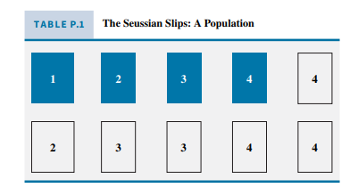
Probability is usually defined in terms of experiments. Let us illustrate this in the context of a simple experiment. Consider the objects in Table P.1 to be a population of interest. In statistics and econometrics, the term population is an important one. A population is a group of objects, such as people, farms, or business firms, having something in common. The population is a complete set and is the focus of an analysis. In this case the population is the set of ten objects shown in Table P.1. Using this population, we will discuss some probability concepts. In an empirical analysis, a sample of observations is collected from the population of interest, and using the sample observations we make inferences about the population.
If we were to select one cell from the table at random (imagine cutting the table into 10 equally sized pieces of paper, stirring them up, and drawing one of the slips without looking), that would constitute a random experiment. Based on this random experiment, we can define several random variables. For example, let the random variable $X$ be the numerical value showing on a slip that we draw. (We use uppercase letters like $X$ to represent random variables in this primer). The term random variable is a bit odd, as it is actually a rule for assigning numerical values to experimental outcomes. In the context of Table P.1, the rule says, “Perform the experiment (stir the slips, and draw one) and for the slip that you obtain assign $X$ to be the number showing.” The values that $X$ can take are denoted by corresponding lowercase letters, $x$, and in this case the values of $X$ are $x=1,2,3$, or 4 .
For the experiment using the population in Table P.1, ${ }^{1}$ we can create a number of random variables. Let $Y$ be a discrete random variable designating the color of the slip, with $Y=1$ denoting
a shaded slip and $Y=0$ denoting a slip with no shading. The numerical values that $Y$ can take are $y=0,1$.
Consider $X$, the numerical value on the slip. If the slips are equally likely to be chosen after shuffling, then in a large number of experiments (i.e., shuffling and drawing one of the slips), $10 \%$ of the time we would observe $X=1,20 \%$ of the time $X=2,30 \%$ of the time $X=3$, and $40 \%$ of the time $X=4$. These are probabilities that the specific values will occur. We would say, for example, $P(X=3)=0.3$. This interpretation is tied to the relative frequency of a particular outcome’s occurring in a large number of experiment replications.
We summarize the probabilities of possible outcomes using a probability density function (pdf). The $p d f$ for a discrete random variable indicates the probability of each possible value occurring. For a discrete random variable $X$ the value of the $p d f f(x)$ is the probability that the random variable $X$ takes the value $x, f(x)=P(X=x)$. Because $f(x)$ is a probability, it must be true that $0 \leq f(x) \leq 1$ and, if $X$ takes $n$ possible values $x_{1}, \ldots, x_{n}$, then the sum of their probabilities must be one
$$
f\left(x_{1}\right)+f\left(x_{2}\right)+\cdots+f\left(x_{n}\right)=1
$$
数学代写|计量经济学原理代写Principles of Econometrics代考|Marginal Distributions
Working with more than one random variable requires a joint probability density function. For the population in Table P.1 we defined two random variables, $X$ the numeric value of a randomly drawn slip and the indicator variable $Y$ that equals 1 if the selected slip is shaded, and 0 if it is not shaded.
Using the joint $p d f$ for $X$ and $Y$ we can say “The probability of selecting a shaded 2 is $0.10 . “$ This is a joint probability because we are talking about the probability of two events occurring simultaneously; the selection takes the value $X=2$ and the slip is shaded so that $Y=1$. We can write this as
$$
P(X=2 \text { and } Y=1)=P(X=2, Y=1)=f(x=2, y=1)=0.1
$$
The entries in Table P.3 are probabilities $f(x, y)=P(X=x, Y=y)$ of joint outcomes. Like the $p d f$ of a single random variable, the sum of the joint probabilities is 1 .
Given a joint $p d f$, we can obtain the probability distributions of individual random variables, which are also known as marginal distributions. In Table P.3, we see that a shaded slip, $Y=1$, can be obtained with the values $x=1,2,3$, and 4 . The probability that we select a shaded slip is the sum of the probabilities that we obtain a shaded 1, a shaded 2, a shaded 3 , and a shaded 4 . The probability that $Y=1$ is
$$
P(Y=1)=f_{Y}(1)=0.1+0.1+0.1+0.1=0.4
$$
This is the sum of the probabilities across the second row of the table. Similarly the probability of drawing a white slip is the sum of the probabilities across the first row of the table, and $P(Y=0)=f_{Y}(0)=0+0.1+0.2+0.3=0.6$, where $f_{Y}(y)$ denotes the $p d f$ of the random variable $Y$. The probabilities $P(X=x)$ are computed similarly by summing down across the values of $Y$. The joint and marginal distributions are often reported as in Table P.4. ${ }^{3}$
计量经济学代考
数学代写|计量经济学原理代写Principles of Econometrics代考|Random Variables
本杰明·富兰克林 (Benjamin Franklin) 有一句名言:“生命中唯一确定的事情就是死亡和税收。” 虽然不是本意,但这一点智慧指出,我们在生活中遇到的几乎所有事情都是不确定的。我们不知道我们的足球队下赛季会赢多少场比赛。你不知道下次考试你会考多少分。我们不知道明天的股市指数会是多少。这些事件或结果是不确定的或随机的。概率为我们提供了一种讨论可能结果的方式。
随机变量是一个变量,其值在被观察之前是未知的;换句话说,它是一个不可完全预测的变量。每个随机变量都有一组它可以取的可能值。如果在是我们足球队明年赢得的比赛数,那么在可以取值0,1,2,…,13, 如果最多有 13 场比赛。这是一个离散随机变量,因为它只能取有限的或可数的值。离散随机变量的其他示例是随机选择的家庭拥有的计算机数量,以及您明年去看医生的次数。当随机变量只能是两个可能值之一时,就会出现一种特殊情况——例如,在电话调查中,如果问你是否是大学毕业生,你的答案只能是“是”或“不是”。 ” 像这样的结果可以通过一个指示变量来表征,如果是,则取值,如果不是,则取零。指标变量是离散的,用于表示诸如性别(男性或女性)或种族(白人或非白人)等定性特征。
美国 GDP 是另一个随机变量的例子,因为它的值在被观察之前是未知的。在 2014 年第三季度,它被计算为16,164.1亿美元。2025年第二季度的价值是多少未知,也无法完美预测。GDP是用美元来衡量的,它可以用整美元来计算,但它的价值是如此之大,以至于计算单个美元是没有用的。出于实际目的,GDP 可以取零到无穷大区间内的任何值,并将其视为连续随机变量。其他常见的宏观经济变量,如利率、投资和消费,也被视为连续随机变量。在金融领域,股票市场指数,如道琼斯工业指数,也被视为连续指数。这些变量使它们连续的关键属性是它们可以在一个区间内取任何值。
数学代写|计量经济学原理代写Principles of Econometrics代考|Probability Distributions
概率通常用实验来定义。让我们通过一个简单的实验来说明这一点。将表 P.1 中的对象视为感兴趣的群体。在统计学和计量经济学中,人口一词是一个重要的术语。人口是一组具有共同点的对象,例如人、农场或商业公司。总体是一个完整的集合,是分析的重点。在这种情况下,总体是表 P.1 中所示的 10 个对象的集合。使用这个总体,我们将讨论一些概率概念。在实证分析中,从感兴趣的总体中收集观察样本,并使用样本观察对总体进行推断。
如果我们从表格中随机选择一个单元格(想象将表格切成 10 张大小相同的纸,搅拌它们,然后不看就画出其中一张纸),这将构成一个随机实验。基于这个随机实验,我们可以定义几个随机变量。例如,让随机变量X是我们绘制的单据上显示的数值。(我们使用大写字母,例如X代表本入门书中的随机变量)。术语随机变量有点奇怪,因为它实际上是为实验结果分配数值的规则。在表 P.1 的上下文中,规则说:“进行实验(搅拌纸条,然后画一张)并为您获得的纸条分配X成为显示的数字。” 那些价值观X可以采取相应的小写字母表示,X,在这种情况下,值X是X=1,2,3, 或 4 .
对于使用表 P.1 中的总体的实验,1我们可以创建许多随机变量。让是是指定滑动颜色的离散随机变量,其中是=1表示
有阴影的滑动和是=0表示没有阴影的滑动。数值是可以带是是=0,1.
考虑X,单据上的数值。如果在洗牌后选择纸条的可能性相同,那么在大量的实验中(即洗牌并绘制其中一张纸条),10%我们观察到的时间X=1,20%的时间X=2,30%的时间X=3, 和40%的时间X=4. 这些是特定值出现的概率。例如,我们会说,磷(X=3)=0.3. 这种解释与大量实验重复中特定结果的相对频率有关。
我们使用概率密度函数 (pdf) 总结可能结果的概率。这pdF对于离散随机变量,表示每个可能值出现的概率。对于离散随机变量X的价值pdFF(X)是随机变量的概率X取值X,F(X)=磷(X=X). 因为F(X)是一个概率,它必须是真的0≤F(X)≤1而如果X需要n可能的值X1,…,Xn, 那么它们的概率之和一定是一
F(X1)+F(X2)+⋯+F(Xn)=1
数学代写|计量经济学原理代写Principles of Econometrics代考|Marginal Distributions
使用多个随机变量需要联合概率密度函数。对于表 P.1 中的总体,我们定义了两个随机变量,X随机抽取的单据的数值和指标变量是如果选定的滑动带阴影,则等于 1,如果不带阴影,则等于 0。
使用关节pdF为了X和是我们可以说“选择阴影 2 的概率是0.10.“这是一个联合概率,因为我们谈论的是两个事件同时发生的概率;选择取值X=2并且滑动是阴影的,因此是=1. 我们可以这样写
磷(X=2 和 是=1)=磷(X=2,是=1)=F(X=2,是=1)=0.1
表 P.3 中的条目是概率F(X,是)=磷(X=X,是=是)的联合成果。像pdF对于单个随机变量,联合概率之和为 1 。
给定一个联合pdF,我们可以得到各个随机变量的概率分布,也称为边际分布。在表 P.3 中,我们看到有阴影的滑动,是=1, 可以用值获得X=1,2,3, 和 4 . 我们选择阴影滑动的概率是我们获得阴影 1、阴影 2、阴影 3 和阴影 4 的概率之和。的概率是=1是
磷(是=1)=F是(1)=0.1+0.1+0.1+0.1=0.4
这是表格第二行的概率之和。类似地,绘制白纸的概率是表格第一行的概率之和,并且磷(是=0)=F是(0)=0+0.1+0.2+0.3=0.6, 在哪里F是(是)表示pdF随机变量是. 概率磷(X=X)类似地通过对是. 联合分布和边际分布通常如表 P.4 所示。3

统计代写请认准statistics-lab™. statistics-lab™为您的留学生涯保驾护航。
金融工程代写
金融工程是使用数学技术来解决金融问题。金融工程使用计算机科学、统计学、经济学和应用数学领域的工具和知识来解决当前的金融问题,以及设计新的和创新的金融产品。
非参数统计代写
非参数统计指的是一种统计方法,其中不假设数据来自于由少数参数决定的规定模型;这种模型的例子包括正态分布模型和线性回归模型。
广义线性模型代考
广义线性模型(GLM)归属统计学领域,是一种应用灵活的线性回归模型。该模型允许因变量的偏差分布有除了正态分布之外的其它分布。
术语 广义线性模型(GLM)通常是指给定连续和/或分类预测因素的连续响应变量的常规线性回归模型。它包括多元线性回归,以及方差分析和方差分析(仅含固定效应)。
有限元方法代写
有限元方法(FEM)是一种流行的方法,用于数值解决工程和数学建模中出现的微分方程。典型的问题领域包括结构分析、传热、流体流动、质量运输和电磁势等传统领域。
有限元是一种通用的数值方法,用于解决两个或三个空间变量的偏微分方程(即一些边界值问题)。为了解决一个问题,有限元将一个大系统细分为更小、更简单的部分,称为有限元。这是通过在空间维度上的特定空间离散化来实现的,它是通过构建对象的网格来实现的:用于求解的数值域,它有有限数量的点。边界值问题的有限元方法表述最终导致一个代数方程组。该方法在域上对未知函数进行逼近。[1] 然后将模拟这些有限元的简单方程组合成一个更大的方程系统,以模拟整个问题。然后,有限元通过变化微积分使相关的误差函数最小化来逼近一个解决方案。
tatistics-lab作为专业的留学生服务机构,多年来已为美国、英国、加拿大、澳洲等留学热门地的学生提供专业的学术服务,包括但不限于Essay代写,Assignment代写,Dissertation代写,Report代写,小组作业代写,Proposal代写,Paper代写,Presentation代写,计算机作业代写,论文修改和润色,网课代做,exam代考等等。写作范围涵盖高中,本科,研究生等海外留学全阶段,辐射金融,经济学,会计学,审计学,管理学等全球99%专业科目。写作团队既有专业英语母语作者,也有海外名校硕博留学生,每位写作老师都拥有过硬的语言能力,专业的学科背景和学术写作经验。我们承诺100%原创,100%专业,100%准时,100%满意。
随机分析代写
随机微积分是数学的一个分支,对随机过程进行操作。它允许为随机过程的积分定义一个关于随机过程的一致的积分理论。这个领域是由日本数学家伊藤清在第二次世界大战期间创建并开始的。
时间序列分析代写
随机过程,是依赖于参数的一组随机变量的全体,参数通常是时间。 随机变量是随机现象的数量表现,其时间序列是一组按照时间发生先后顺序进行排列的数据点序列。通常一组时间序列的时间间隔为一恒定值(如1秒,5分钟,12小时,7天,1年),因此时间序列可以作为离散时间数据进行分析处理。研究时间序列数据的意义在于现实中,往往需要研究某个事物其随时间发展变化的规律。这就需要通过研究该事物过去发展的历史记录,以得到其自身发展的规律。
回归分析代写
多元回归分析渐进(Multiple Regression Analysis Asymptotics)属于计量经济学领域,主要是一种数学上的统计分析方法,可以分析复杂情况下各影响因素的数学关系,在自然科学、社会和经济学等多个领域内应用广泛。
MATLAB代写
MATLAB 是一种用于技术计算的高性能语言。它将计算、可视化和编程集成在一个易于使用的环境中,其中问题和解决方案以熟悉的数学符号表示。典型用途包括:数学和计算算法开发建模、仿真和原型制作数据分析、探索和可视化科学和工程图形应用程序开发,包括图形用户界面构建MATLAB 是一个交互式系统,其基本数据元素是一个不需要维度的数组。这使您可以解决许多技术计算问题,尤其是那些具有矩阵和向量公式的问题,而只需用 C 或 Fortran 等标量非交互式语言编写程序所需的时间的一小部分。MATLAB 名称代表矩阵实验室。MATLAB 最初的编写目的是提供对由 LINPACK 和 EISPACK 项目开发的矩阵软件的轻松访问,这两个项目共同代表了矩阵计算软件的最新技术。MATLAB 经过多年的发展,得到了许多用户的投入。在大学环境中,它是数学、工程和科学入门和高级课程的标准教学工具。在工业领域,MATLAB 是高效研究、开发和分析的首选工具。MATLAB 具有一系列称为工具箱的特定于应用程序的解决方案。对于大多数 MATLAB 用户来说非常重要,工具箱允许您学习和应用专业技术。工具箱是 MATLAB 函数(M 文件)的综合集合,可扩展 MATLAB 环境以解决特定类别的问题。可用工具箱的领域包括信号处理、控制系统、神经网络、模糊逻辑、小波、仿真等。