如果你也在 怎样代写黎曼几何Riemannian geometry这个学科遇到相关的难题,请随时右上角联系我们的24/7代写客服。
黎曼几何是研究黎曼流形的微分几何学分支,黎曼流形是具有黎曼公制的光滑流形,即在每一点的切线空间上有一个内积,从一点到另一点平滑变化。
statistics-lab™ 为您的留学生涯保驾护航 在代写黎曼几何Riemannian geometry方面已经树立了自己的口碑, 保证靠谱, 高质且原创的统计Statistics代写服务。我们的专家在代写黎曼几何Riemannian geometry代写方面经验极为丰富,各种代写黎曼几何Riemannian geometry相关的作业也就用不着说。
我们提供的黎曼几何Riemannian geometry及其相关学科的代写,服务范围广, 其中包括但不限于:
- Statistical Inference 统计推断
- Statistical Computing 统计计算
- Advanced Probability Theory 高等概率论
- Advanced Mathematical Statistics 高等数理统计学
- (Generalized) Linear Models 广义线性模型
- Statistical Machine Learning 统计机器学习
- Longitudinal Data Analysis 纵向数据分析
- Foundations of Data Science 数据科学基础
数学代写|黎曼几何代写Riemannian geometry代考|Geodesics and Optimality
Let $M \subset \mathbb{R}^{3}$ be a surface and $\gamma:[0, T] \rightarrow M$ be a smooth curve in $M$. The length of $\gamma$ is defined as
$$
\ell(\gamma):=\int_{0}^{T}|\dot{\gamma}(t)| d t,
$$
where $|v|=\sqrt{\langle v \mid v\rangle}$ denotes the norm of a vector $v$ in $\mathbb{R}^{3}$.
Notice that the definition of length in (1.1) is invariant under reparametrizations of the curve. Indeed, let $\varphi:\left[0, T^{\prime}\right] \rightarrow[0, T]$ be a smooth monotonic function. Define $\gamma_{\varphi}:\left[0, T^{\prime}\right] \rightarrow M$ by $\gamma_{\varphi}:=\gamma \circ \varphi$. Using the change of variables $t=\varphi(s)$, one gets
$$
\ell\left(\gamma_{\varphi}\right)=\int_{0}^{T^{\prime}}\left|\dot{\gamma}{\varphi}(s)\right| d s=\int{0}^{T^{\prime}}|\dot{\gamma}(\varphi(s))||\dot{\varphi}(s)| d s=\int_{0}^{T}|\dot{\gamma}(t)| d t=\ell(\gamma) .
$$
The definition of length can be extended to piecewise-smooth curves on $M$ by adding the length of every smooth piece of $\gamma$.
When the curve $\gamma$ is parametrized in such a way that $|\dot{\gamma}(t)| \equiv c$ for some $c>0$ we say that $\gamma$ has constant speed. If moreover $c=1$, we say that $\gamma$ is parametrized by arclength (or arclength parametrized).
The distance between two points $p, q \in M$ is the infimum of the lengths of curves that join $p$ to $q$ :
$d(p, q)=\inf {\ell(\gamma) \mid \gamma:[0, T] \rightarrow M$ piecewise-smooth, $\gamma(0)=p, \gamma(T)=q}$
Now we focus on length-minimizers, i.e., piecewise-smooth curves $\gamma:[0, T]$ $\rightarrow M$ realizing the distance between their endpoints, i.e., satisfying $\ell(\gamma)=$ $d(\gamma(0), \gamma(T))$.
数学代写|黎曼几何代写Riemannian geometry代考|Existence and Minimizing Properties of Geodesics
As a direct consequence of Proposition $1.8$ one obtains the following existence and uniqueness theorem for geodesics.
Corollary 1.10 Let $q \in M$ and $v \in T_{q} M$. There exists a unique geodesic $\gamma:[0, \varepsilon] \rightarrow M$, for $\varepsilon>0$ small enough, such that $\gamma(0)=q$ and $\dot{\gamma}(0)=v$.
Proof By Proposition 1.8, geodesics satisfy a second-order ordinary differential equation (ODE), hence they are smooth curves characterized by their initial position and velocity.
To end this section we show that small pieces of geodesics are always global minimizers.
Theorem 1.11 Let $\gamma:[0, T] \rightarrow M$ be a geodesic. For every $\tau \in[0, T[$ there exists $\varepsilon>0$ such that
(i) $\left.\gamma\right|{[\tau, \tau+\varepsilon]}$ is a minimizer, i.e., $d(\gamma(\tau), \gamma(\tau+\varepsilon))=\ell\left(\left.\gamma\right|{[\tau, \tau+\varepsilon]}\right)$,
(ii) $\left.\gamma\right|_{[\tau, \tau+\varepsilon]}$ is the unique minimizer joining $\gamma(\tau)$ and $\gamma(\tau+\varepsilon)$ in the class of piecewise-smooth curves, up to reparametrization.
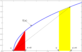
Proof Without loss of generality let us assume that $\tau=0$ and that $\gamma$ is arclength parametrized. Consider an arclength parametrized curve $\alpha$ on $M$, such that $\alpha(0)=\gamma(0)$ and $\dot{\alpha}(0) \perp \dot{\gamma}(0)$, and denote by $(t, s) \mapsto x_{s}(t)$ a smooth variation of geodesics such that $x_{0}(t)=\gamma(t)$ and (see also Figure 1.1)
$$
x_{s}(0)=\alpha(s), \quad \dot{x}{s}(0) \perp \frac{\partial}{\partial s} \alpha(s) . $$ The map $\psi:(t, s) \mapsto x{s}(t)$ is smooth and is a local diffeomorphism near $(0,0)$. Indeed, we can compute the partial derivatives
$$
\left.\frac{\partial \psi}{\partial t}\right|{t=s=0}=\left.\frac{\partial}{\partial t}\right|{t=0} x_{0}(t)=\dot{\gamma}(0),\left.\quad \frac{\partial \psi}{\partial s}\right|{t=s=0}=\left.\frac{\partial}{\partial s}\right|{s=0} x_{s}(0)=\dot{\alpha}(0),
$$
and they are linearly independent. Thus $\psi$ maps a neighborhood $U$ of $(0,0)$ to a neighbōthood $W$ of $\gamma(0)$. We now considèr a function $\phi$ and a vecctor field $X$ defined on $W$ by
$$
\phi: x_{s}(t) \mapsto t, \quad X: x_{s}(t) \mapsto \dot{x}_{s}(t)
$$
数学代写|黎曼几何代写Riemannian geometry代考|Absolutely Continuous Curves
Notice that formula (1.1) defines the length of a curve even if $\gamma$ is only absolutely continuous, if one interprets the integral in the Lebesgue sense (recall that absolutely continuous curves are differentiable almost everywhere).
The proof of Theorem $1.11$, and in particular estimates (1.20) and (1.21), can be extended to the class of absolutely continuous curves. This proves that small pieces of geodesics are also minimizers in the larger class of absolutely continuous curves on $M$. As a byproduct, we have the following corollary.
Corollary $1.13$ Any length-minimizer (in the class of absolutely continuous curves) is a geodesic, and hence smooth.
In this section we want to introduce the notion of parallel transport on a surface (along a curve), which allows us to define its main geometric invariant: the Gaussian curvature.
Definition 1.14 Let $\gamma:[0, T] \rightarrow M$ be a smooth curve. A smooth curve of tangent vectors $\xi(t) \in T_{\gamma(t)} M$ is said to be parallel if $\dot{\xi}(t) \perp T_{\gamma(t)} M$.
This notion generalizes the notion of parallelism of vectors on the plane, where it is possible to canonically identify every tangent space to $M=\mathbb{R}^{2}$ with $\mathbb{R}^{2}$ itself. ${ }^{2}$ In this case a smooth curve of tangent vectors $\xi(t) \in T_{\gamma(t)} M$ is parallel if and only if $\dot{\xi}(t)=0$.
When $M$ is the zero level of a smooth function $a: \mathbb{R}^{3} \rightarrow \mathbb{R}$, as in (1.14), we have the following description:
Proposition $1.15$ A smooth curve of tangent vectors $\xi(t)$ defined along $\gamma:[0, T] \rightarrow M$ is parallel if and only if it satisfies
$$
\dot{\xi}(t)=-\frac{\dot{\gamma}(t)^{T}\left(\nabla_{\gamma(t)}^{2} a\right) \xi(t)}{\left|\nabla_{\gamma(t)} a\right|^{2}} \nabla_{\gamma(t)} a, \quad \forall t \in[0, T] .
$$
Proof As in Remark 1.7, $\xi(t) \in T_{\gamma(t)} M$ implies that $\left\langle\nabla_{\gamma(t)} a, \xi(t)\right\rangle=0$. Moreover, by assumption, $\dot{\xi}(t)=\alpha(t) \nabla_{\gamma(t)} a$ for some smooth function $\alpha$. With computations analogous to those in the proof of Proposition $1.8$ we get that
$$
\dot{\gamma}(t)^{T}\left(\nabla_{\gamma(t)}^{2} a\right) \xi(t)+\alpha(t)\left|\nabla_{\gamma(t)} a\right|^{2}=0,
$$
from which the statement follows.
黎曼几何代考
数学代写|黎曼几何代写Riemannian geometry代考|Geodesics and Optimality
让米⊂R3是一个表面并且C:[0,吨]→米成为一条平滑的曲线米. 的长度C定义为
ℓ(C):=∫0吨|C˙(吨)|d吨,
在哪里|在|=⟨在∣在⟩表示向量的范数在在R3.
请注意,(1.1) 中的长度定义在曲线的重新参数化下是不变的。确实,让披:[0,吨′]→[0,吨]是一个光滑的单调函数。定义C披:[0,吨′]→米经过C披:=C∘披. 使用变量的变化吨=披(s), 得到
$$
\ell\left(\gamma_{\varphi}\right)=\int_{0}^{T^{\prime}}\left|\dot{\gamma} {\varphi}(s) \对| ds=\int {0}^{T^{\prime}}|\dot{\gamma}(\varphi(s))||\dot{\varphi}(s)| ds=\int_{0}^{T}|\dot{\gamma}(t)| dt=\ell(\gamma) 。
$$
长度的定义可以扩展到分段平滑曲线米通过添加每个光滑部分的长度C.
当曲线C以这样的方式参数化|C˙(吨)|≡C对于一些C>0我们说C有恒定的速度。此外,如果C=1, 我们说C由 arclength 参数化(或 arclength 参数化)。
两点之间的距离p,q∈米是连接的曲线长度的下确界p至q :
d(p,q)=信息ℓ(C)∣C:[0,吨]→米$p一世和C和在一世s和−s米○○吨H,$C(0)=p,C(吨)=q
现在我们关注长度最小化器,即分段平滑曲线C:[0,吨] →米实现它们的端点之间的距离,即满足ℓ(C)= d(C(0),C(吨)).
数学代写|黎曼几何代写Riemannian geometry代考|Existence and Minimizing Properties of Geodesics
作为命题的直接结果1.8可以得到以下测地线存在性和唯一性定理。
推论 1.10 让q∈米和在∈吨q米. 存在独特的测地线C:[0,e]→米, 为了e>0足够小,这样C(0)=q和C˙(0)=在.
由命题 1.8 证明,测地线满足二阶常微分方程 (ODE),因此它们是以其初始位置和速度为特征的平滑曲线。
在本节结束时,我们将展示小块测地线始终是全局最小化器。
定理 1.11 让C:[0,吨]→米做一个测地线。对于每一个τ∈[0,吨[那里存在e>0这样
(i)C|[τ,τ+e]是一个极小值,即d(C(τ),C(τ+e))=ℓ(C|[τ,τ+e]),
(ii)C|[τ,τ+e]是唯一的最小化器加入C(τ)和C(τ+e)在分段平滑曲线的类中,直到重新参数化。
证明 不失一般性让我们假设τ=0然后C是弧长参数化的。考虑弧长参数化曲线一个上米, 这样一个(0)=C(0)和一个˙(0)⊥C˙(0),并表示为(吨,s)↦Xs(吨)测地线的平滑变化,使得X0(吨)=C(吨)和(另请参见图 1.1)
Xs(0)=一个(s),X˙s(0)⊥∂∂s一个(s).地图ψ:(吨,s)↦Xs(吨)是光滑的并且是附近的局部微分同胚(0,0). 事实上,我们可以计算偏导数
∂ψ∂吨|吨=s=0=∂∂吨|吨=0X0(吨)=C˙(0),∂ψ∂s|吨=s=0=∂∂s|s=0Xs(0)=一个˙(0),
并且它们是线性独立的。因此ψ映射一个社区在的(0,0)到一个街区在的C(0). 我们现在考虑一个函数φ和一个向量场X定义于在经过
φ:Xs(吨)↦吨,X:Xs(吨)↦X˙s(吨)
数学代写|黎曼几何代写Riemannian geometry代考|Absolutely Continuous Curves
请注意,公式 (1.1) 定义了曲线的长度,即使C仅是绝对连续的,如果以 Lebesgue 意义来解释积分(回想一下,绝对连续曲线几乎处处可微)。
定理的证明1.11,特别是估计(1.20)和(1.21),可以扩展到绝对连续曲线的类别。这证明了在更大的绝对连续曲线类别中,小块测地线也是极小值。米. 作为副产品,我们有以下推论。
推论1.13任何长度最小化器(在绝对连续曲线类中)都是测地线,因此是平滑的。
在本节中,我们要介绍表面(沿曲线)上的平行传输的概念,它允许我们定义其主要的几何不变量:高斯曲率。
定义 1.14 让C:[0,吨]→米成为一条平滑的曲线。切向量的平滑曲线X(吨)∈吨C(吨)米据说是平行的,如果X˙(吨)⊥吨C(吨)米.
这个概念概括了平面上向量平行度的概念,其中可以规范地识别每个切线空间米=R2和R2本身。2在这种情况下,切向量的平滑曲线X(吨)∈吨C(吨)米当且仅当是平行的X˙(吨)=0.
什么时候米是平滑函数的零水平一个:R3→R,如(1.14)中,我们有以下描述:
主张1.15切向量的平滑曲线X(吨)沿定义C:[0,吨]→米当且仅当它满足时是平行的
X˙(吨)=−C˙(吨)吨(∇C(吨)2一个)X(吨)|∇C(吨)一个|2∇C(吨)一个,∀吨∈[0,吨].
证明 如备注 1.7,X(吨)∈吨C(吨)米暗示⟨∇C(吨)一个,X(吨)⟩=0. 此外,根据假设,X˙(吨)=一个(吨)∇C(吨)一个对于一些平滑的功能一个. 计算类似于命题证明中的计算1.8我们明白了
C˙(吨)吨(∇C(吨)2一个)X(吨)+一个(吨)|∇C(吨)一个|2=0,
声明如下。

统计代写请认准statistics-lab™. statistics-lab™为您的留学生涯保驾护航。
金融工程代写
金融工程是使用数学技术来解决金融问题。金融工程使用计算机科学、统计学、经济学和应用数学领域的工具和知识来解决当前的金融问题,以及设计新的和创新的金融产品。
非参数统计代写
非参数统计指的是一种统计方法,其中不假设数据来自于由少数参数决定的规定模型;这种模型的例子包括正态分布模型和线性回归模型。
广义线性模型代考
广义线性模型(GLM)归属统计学领域,是一种应用灵活的线性回归模型。该模型允许因变量的偏差分布有除了正态分布之外的其它分布。
术语 广义线性模型(GLM)通常是指给定连续和/或分类预测因素的连续响应变量的常规线性回归模型。它包括多元线性回归,以及方差分析和方差分析(仅含固定效应)。
有限元方法代写
有限元方法(FEM)是一种流行的方法,用于数值解决工程和数学建模中出现的微分方程。典型的问题领域包括结构分析、传热、流体流动、质量运输和电磁势等传统领域。
有限元是一种通用的数值方法,用于解决两个或三个空间变量的偏微分方程(即一些边界值问题)。为了解决一个问题,有限元将一个大系统细分为更小、更简单的部分,称为有限元。这是通过在空间维度上的特定空间离散化来实现的,它是通过构建对象的网格来实现的:用于求解的数值域,它有有限数量的点。边界值问题的有限元方法表述最终导致一个代数方程组。该方法在域上对未知函数进行逼近。[1] 然后将模拟这些有限元的简单方程组合成一个更大的方程系统,以模拟整个问题。然后,有限元通过变化微积分使相关的误差函数最小化来逼近一个解决方案。
tatistics-lab作为专业的留学生服务机构,多年来已为美国、英国、加拿大、澳洲等留学热门地的学生提供专业的学术服务,包括但不限于Essay代写,Assignment代写,Dissertation代写,Report代写,小组作业代写,Proposal代写,Paper代写,Presentation代写,计算机作业代写,论文修改和润色,网课代做,exam代考等等。写作范围涵盖高中,本科,研究生等海外留学全阶段,辐射金融,经济学,会计学,审计学,管理学等全球99%专业科目。写作团队既有专业英语母语作者,也有海外名校硕博留学生,每位写作老师都拥有过硬的语言能力,专业的学科背景和学术写作经验。我们承诺100%原创,100%专业,100%准时,100%满意。
随机分析代写
随机微积分是数学的一个分支,对随机过程进行操作。它允许为随机过程的积分定义一个关于随机过程的一致的积分理论。这个领域是由日本数学家伊藤清在第二次世界大战期间创建并开始的。
时间序列分析代写
随机过程,是依赖于参数的一组随机变量的全体,参数通常是时间。 随机变量是随机现象的数量表现,其时间序列是一组按照时间发生先后顺序进行排列的数据点序列。通常一组时间序列的时间间隔为一恒定值(如1秒,5分钟,12小时,7天,1年),因此时间序列可以作为离散时间数据进行分析处理。研究时间序列数据的意义在于现实中,往往需要研究某个事物其随时间发展变化的规律。这就需要通过研究该事物过去发展的历史记录,以得到其自身发展的规律。
回归分析代写
多元回归分析渐进(Multiple Regression Analysis Asymptotics)属于计量经济学领域,主要是一种数学上的统计分析方法,可以分析复杂情况下各影响因素的数学关系,在自然科学、社会和经济学等多个领域内应用广泛。
MATLAB代写
MATLAB 是一种用于技术计算的高性能语言。它将计算、可视化和编程集成在一个易于使用的环境中,其中问题和解决方案以熟悉的数学符号表示。典型用途包括:数学和计算算法开发建模、仿真和原型制作数据分析、探索和可视化科学和工程图形应用程序开发,包括图形用户界面构建MATLAB 是一个交互式系统,其基本数据元素是一个不需要维度的数组。这使您可以解决许多技术计算问题,尤其是那些具有矩阵和向量公式的问题,而只需用 C 或 Fortran 等标量非交互式语言编写程序所需的时间的一小部分。MATLAB 名称代表矩阵实验室。MATLAB 最初的编写目的是提供对由 LINPACK 和 EISPACK 项目开发的矩阵软件的轻松访问,这两个项目共同代表了矩阵计算软件的最新技术。MATLAB 经过多年的发展,得到了许多用户的投入。在大学环境中,它是数学、工程和科学入门和高级课程的标准教学工具。在工业领域,MATLAB 是高效研究、开发和分析的首选工具。MATLAB 具有一系列称为工具箱的特定于应用程序的解决方案。对于大多数 MATLAB 用户来说非常重要,工具箱允许您学习和应用专业技术。工具箱是 MATLAB 函数(M 文件)的综合集合,可扩展 MATLAB 环境以解决特定类别的问题。可用工具箱的领域包括信号处理、控制系统、神经网络、模糊逻辑、小波、仿真等。