标签: MTH 3022

数学代写|黎曼曲面代写Riemann surface代考|Elliptic functions

如果你也在 怎样代写黎曼曲面Riemann surface这个学科遇到相关的难题,请随时右上角联系我们的24/7代写客服。

黎曼曲面是一个类似于曲面的构型,它在复平面上覆盖着几个,一般来说是无限多的 “片”。这些薄片可以有非常复杂的结构和相互的联系。

statistics-lab™ 为您的留学生涯保驾护航 在代写黎曼曲面Riemann surface方面已经树立了自己的口碑, 保证靠谱, 高质且原创的统计Statistics代写服务。我们的专家在代写黎曼曲面Riemann surface代写方面经验极为丰富,各种代写黎曼曲面Riemann surface相关的作业也就用不着说。

我们提供的黎曼曲面Riemann surface及其相关学科的代写,服务范围广, 其中包括但不限于:

  • Statistical Inference 统计推断
  • Statistical Computing 统计计算
  • Advanced Probability Theory 高等概率论
  • Advanced Mathematical Statistics 高等数理统计学
  • (Generalized) Linear Models 广义线性模型
  • Statistical Machine Learning 统计机器学习
  • Longitudinal Data Analysis 纵向数据分析
  • Foundations of Data Science 数据科学基础
数学代写|黎曼曲面代写Riemann surface代考|Elliptic functions

数学代写|黎曼曲面代写Riemann surface代考|Elliptic functions

We now turn to the study of meromorphic functions on Riemann surfaces of genus 1 .
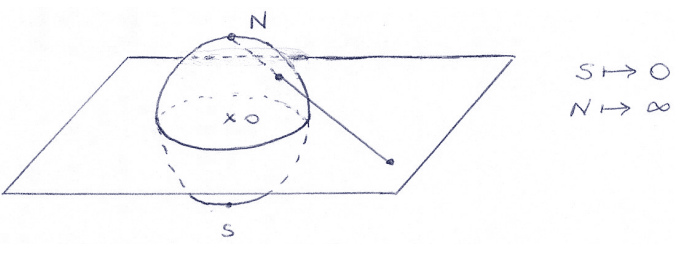
The only Riemann surface of genus 0 is the Riemann sphere $\mathbb{P}^1=\mathbb{C} \cup{\infty}$. (This is not obvious: we are saying that any abstract Riemann surface structure on the 2 -sphere ends up being isomorphic to the standard one. If you recall hat Riemann surface structures can be defined by gluing, you see why this is not a simple consequence of any definition). On $\mathbb{P}^1$, the meromorphic functions are rational, and those we understand quite explicitly; so it is natural to study tori next.

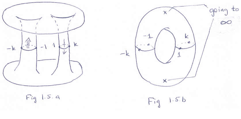
The tori we shall study are of the form $\mathbb{C} / L$, where $L \subset \mathbb{C}$ is a lattice – a free abelian subgroup for which the quotient is a topological torus. A less tautological definition is, viewing $\mathbb{C}$ as $\mathbb{R}^2$, that $L$ should be generated over $\mathbb{Z}$ by two vectors which are not parallel. Calling them $\omega_1$ and $\omega_2$, the conditions are
$$
\omega_1, \omega_2 \neq 0 \quad \text { and } \quad \frac{\omega_1}{\omega_2} \notin \mathbb{R} \text {. }
$$’

8.1 Exercise: Show, if $\omega_1 / \omega_2 \in \mathbb{R}$, that $\mathbb{Z} \omega_1+\mathbb{Z} \omega_2 \subset \mathbb{C}$ is either generated over $\mathbb{Z}$ by a single vector, or else its points are dense on a line. (The two cases correspond to $\omega_1 / \omega_2 \in \mathbb{Q}$ and $\omega_1 / \omega_2 \in \mathbb{R} \backslash \mathbb{Q}$.)

By definition, a function $f$ is holomorphic on an open subset $U \subseteq \mathbb{C} / L$ iff $f \circ \pi$ is holomorphic on $\pi^{-1}(U) \subseteq \mathbb{C}$, where $\pi: \mathbb{C} \rightarrow \mathbb{C} / L$ is the projection.
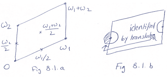
Note that a ‘fundamental domain’ for the action of $L$ on $\mathbb{C}$ is the ‘period parallelogram’ Strictly speaking, to represent each point only once, we should take the interior of the parallelogram, two open edges and a single vertex; but it is more sensible to view $\mathbb{C} / L$ as arising from the closed parallelogram by identifying opposite sides. The notion of holomorphicity is pictorially clear now, even at a boundary point $P$ – we require matching functions on the two halfneighbourhoods of $P$.

数学代写|黎曼曲面代写Riemann surface代考|Remark

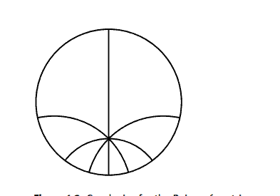
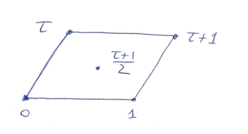
8.2 Remark: Division by $\omega_1$ turns the period parallelogram into the form depicted in Fig. 8.2, with $\tau=\omega_2 / \omega_1 \notin \mathbb{R}$.

Another presentation of the Riemann surface $T=\mathbb{C} / L$ is then visibly as $\mathbb{C}^* / \mathbb{Z}$, where the abelian group $\mathbb{Z}$ is identified with the multiplicative subgroup of $\mathbb{C}^$ generated by $q=e^{\pi i \tau}$. We have a map $\exp : \mathbb{C} \rightarrow \mathbb{C}^$ which descends to an isomorphism of Riemann surfaces, between $\mathbb{C} / L$ and $\mathbb{C}^* /\left{q^{\mathbb{Z}}\right}$

Returning to the $\mathbb{C} / L$ description, we see that functions on $T$ correspond to doubly periodic functions on $\mathbb{C}$, that is, functions satisfying
$$
f\left(u+\omega_1\right)=f\left(u+\omega_2\right)=f(u)
$$
for all $u \in \mathbb{C}$. For starters, we note the following:
8.3 Proposition: Any doubly periodic holomorphic function on $\mathbb{C}$ is constant.
First Proof: Global holomorphic functions on $\mathbb{C} / L$ are constant.
Second Proof: By Liouville’s theorem, bounded holomorphic functions on $\mathbb{C}$ are constant.

8.4 Definition: An elliptic function is a doubly periodic meromorphic function on $\mathbb{C}$.
Elliptic functions are thus meromorphic functions on a torus $\mathbb{C} / L$. The reason for the name is lost in the dawn of time. (Really, elliptic functions can be used to express the arc-length on the ellipse.)

Constructing the first example of an elliptic function takes some work. We shall in fact describe them all; but we must start with some generalities.
8.5 Theorem: Let $z_1, \ldots, z_n$ and $p_1, \ldots, p_m$ denote the zeroes and poles of a non-constant elliptic function $f$ in the period parallelogram, repeated according to multiplicity. Then:
(i) $m=n$,
(ii) $\sum_{k=1}^m \operatorname{Res}{p_k}(f)=0$, (iii) $\sum{k=1}^n z_k=\sum_{k=1}^m p_k(\bmod L)$.

数学代写|黎曼曲面代写Riemann surface代考|Elliptic functions

黎曼曲面代考

数学代写|黎曼曲面代写Riemann surface代考|Elliptic functions

现在我们转向研究属1的黎曼曲面上的亚纯函数。
唯一的属0的黎曼曲面是黎曼球$\mathbb{P}^1=\mathbb{C} \cup{\infty}$。(这并不明显:我们说的是2球上的任何抽象黎曼表面结构最终都与标准黎曼表面结构同构。如果你回想一下黎曼表面结构可以通过粘合来定义,你就会明白为什么这不是任何定义的简单结果)。在$\mathbb{P}^1$上,亚纯函数是有理数,我们很清楚地理解;所以接下来自然要研究tori。

我们将研究的环面是$\mathbb{C} / L$的形式,其中$L \subset \mathbb{C}$是一个格——一个自由的阿贝尔子群,其商是一个拓扑环面。一个较少重复的定义是,将$\mathbb{C}$看作$\mathbb{R}^2$, $L$应该由两个不平行的向量在$\mathbb{Z}$上生成。将它们称为$\omega_1$和$\omega_2$,条件是
$$
\omega_1, \omega_2 \neq 0 \quad \text { and } \quad \frac{\omega_1}{\omega_2} \notin \mathbb{R} \text {. }
$$”

8.1练习:如果$\omega_1 / \omega_2 \in \mathbb{R}$,表示$\mathbb{Z} \omega_1+\mathbb{Z} \omega_2 \subset \mathbb{C}$是由单个向量在$\mathbb{Z}$上生成的,否则它的点在一条线上是密集的。(这两种情况对应于$\omega_1 / \omega_2 \in \mathbb{Q}$和$\omega_1 / \omega_2 \in \mathbb{R} \backslash \mathbb{Q}$。)

根据定义,函数$f$在开放子集$U \subseteq \mathbb{C} / L$上是全纯的,如果$f \circ \pi$在$\pi^{-1}(U) \subseteq \mathbb{C}$上是全纯的,其中$\pi: \mathbb{C} \rightarrow \mathbb{C} / L$是投影。
请注意,$L$作用于$\mathbb{C}$的“基本域”是“周期平行四边形”严格来说,为了表示每个点一次,我们应该取平行四边形的内部,两条开放的边和一个顶点;但更明智的做法是,通过确定对边,将$\mathbb{C} / L$看作是由封闭的平行四边形产生的。现在全纯性的概念在图像上已经很清楚了,即使在边界点$P$ -我们需要在$P$的两个半邻域上匹配函数。

数学代写|黎曼曲面代写Riemann surface代考|Remark

8.2注:除以$\omega_1$,周期平行四边形得到图8.2所示的形式,其中有$\tau=\omega_2 / \omega_1 \notin \mathbb{R}$。

黎曼曲面$T=\mathbb{C} / L$的另一种表示形式可见为$\mathbb{C}^* / \mathbb{Z}$,其中阿贝尔群$\mathbb{Z}$与$q=e^{\pi i \tau}$生成的$\mathbb{C}^$的乘法子群相识别。我们有一个映射$\exp : \mathbb{C} \rightarrow \mathbb{C}^$它下降到黎曼曲面的同构,在$\mathbb{C} / L$和 $\mathbb{C}^* /\left{q^{\mathbb{Z}}\right}$

回到$\mathbb{C} / L$描述,我们看到$T$上的函数对应于$\mathbb{C}$上的双周期函数,也就是说,函数满足
$$
f\left(u+\omega_1\right)=f\left(u+\omega_2\right)=f(u)
$$
对于所有$u \in \mathbb{C}$。对于初学者,我们注意到以下几点:
8.3命题:$\mathbb{C}$上的任何双周期全纯函数都是常数。
第一个证明:$\mathbb{C} / L$上的全局全纯函数是常数。
第二个证明:利用Liouville定理,$\mathbb{C}$上的有界全纯函数是常数。

8.4定义:椭圆函数是$\mathbb{C}$上的双周期亚纯函数。
因此椭圆函数是环面上的亚纯函数$\mathbb{C} / L$。这个名字的由来在时间的黎明中消失了。(实际上,椭圆函数可以用来表示椭圆上的弧长。)

构造椭圆函数的第一个例子需要做一些工作。事实上,我们将一一描述;但我们必须从一些概括性的东西开始。
8.5定理:设$z_1, \ldots, z_n$和$p_1, \ldots, p_m$为周期平行四边形中一个非常椭圆函数$f$的零点和极点,按多重重复。然后:
(i) $m=n$;
(ii) $\sum_{k=1}^m \operatorname{Res}{p_k}(f)=0$, (iii) $\sum{k=1}^n z_k=\sum_{k=1}^m p_k(\bmod L)$。

数学代写|黎曼曲面代写Riemann surface代考 请认准statistics-lab™

统计代写请认准statistics-lab™. statistics-lab™为您的留学生涯保驾护航。

金融工程代写

金融工程是使用数学技术来解决金融问题。金融工程使用计算机科学、统计学、经济学和应用数学领域的工具和知识来解决当前的金融问题,以及设计新的和创新的金融产品。

非参数统计代写

非参数统计指的是一种统计方法,其中不假设数据来自于由少数参数决定的规定模型;这种模型的例子包括正态分布模型和线性回归模型。

广义线性模型代考

广义线性模型(GLM)归属统计学领域,是一种应用灵活的线性回归模型。该模型允许因变量的偏差分布有除了正态分布之外的其它分布。

术语 广义线性模型(GLM)通常是指给定连续和/或分类预测因素的连续响应变量的常规线性回归模型。它包括多元线性回归,以及方差分析和方差分析(仅含固定效应)。

有限元方法代写

有限元方法(FEM)是一种流行的方法,用于数值解决工程和数学建模中出现的微分方程。典型的问题领域包括结构分析、传热、流体流动、质量运输和电磁势等传统领域。

有限元是一种通用的数值方法,用于解决两个或三个空间变量的偏微分方程(即一些边界值问题)。为了解决一个问题,有限元将一个大系统细分为更小、更简单的部分,称为有限元。这是通过在空间维度上的特定空间离散化来实现的,它是通过构建对象的网格来实现的:用于求解的数值域,它有有限数量的点。边界值问题的有限元方法表述最终导致一个代数方程组。该方法在域上对未知函数进行逼近。[1] 然后将模拟这些有限元的简单方程组合成一个更大的方程系统,以模拟整个问题。然后,有限元通过变化微积分使相关的误差函数最小化来逼近一个解决方案。

tatistics-lab作为专业的留学生服务机构,多年来已为美国、英国、加拿大、澳洲等留学热门地的学生提供专业的学术服务,包括但不限于Essay代写,Assignment代写,Dissertation代写,Report代写,小组作业代写,Proposal代写,Paper代写,Presentation代写,计算机作业代写,论文修改和润色,网课代做,exam代考等等。写作范围涵盖高中,本科,研究生等海外留学全阶段,辐射金融,经济学,会计学,审计学,管理学等全球99%专业科目。写作团队既有专业英语母语作者,也有海外名校硕博留学生,每位写作老师都拥有过硬的语言能力,专业的学科背景和学术写作经验。我们承诺100%原创,100%专业,100%准时,100%满意。

随机分析代写


随机微积分是数学的一个分支,对随机过程进行操作。它允许为随机过程的积分定义一个关于随机过程的一致的积分理论。这个领域是由日本数学家伊藤清在第二次世界大战期间创建并开始的。

时间序列分析代写

随机过程,是依赖于参数的一组随机变量的全体,参数通常是时间。 随机变量是随机现象的数量表现,其时间序列是一组按照时间发生先后顺序进行排列的数据点序列。通常一组时间序列的时间间隔为一恒定值(如1秒,5分钟,12小时,7天,1年),因此时间序列可以作为离散时间数据进行分析处理。研究时间序列数据的意义在于现实中,往往需要研究某个事物其随时间发展变化的规律。这就需要通过研究该事物过去发展的历史记录,以得到其自身发展的规律。

回归分析代写

多元回归分析渐进(Multiple Regression Analysis Asymptotics)属于计量经济学领域,主要是一种数学上的统计分析方法,可以分析复杂情况下各影响因素的数学关系,在自然科学、社会和经济学等多个领域内应用广泛。

MATLAB代写

MATLAB 是一种用于技术计算的高性能语言。它将计算、可视化和编程集成在一个易于使用的环境中,其中问题和解决方案以熟悉的数学符号表示。典型用途包括:数学和计算算法开发建模、仿真和原型制作数据分析、探索和可视化科学和工程图形应用程序开发,包括图形用户界面构建MATLAB 是一个交互式系统,其基本数据元素是一个不需要维度的数组。这使您可以解决许多技术计算问题,尤其是那些具有矩阵和向量公式的问题,而只需用 C 或 Fortran 等标量非交互式语言编写程序所需的时间的一小部分。MATLAB 名称代表矩阵实验室。MATLAB 最初的编写目的是提供对由 LINPACK 和 EISPACK 项目开发的矩阵软件的轻松访问,这两个项目共同代表了矩阵计算软件的最新技术。MATLAB 经过多年的发展,得到了许多用户的投入。在大学环境中,它是数学、工程和科学入门和高级课程的标准教学工具。在工业领域,MATLAB 是高效研究、开发和分析的首选工具。MATLAB 具有一系列称为工具箱的特定于应用程序的解决方案。对于大多数 MATLAB 用户来说非常重要,工具箱允许您学习应用专业技术。工具箱是 MATLAB 函数(M 文件)的综合集合,可扩展 MATLAB 环境以解决特定类别的问题。可用工具箱的领域包括信号处理、控制系统、神经网络、模糊逻辑、小波、仿真等。

R语言代写问卷设计与分析代写
PYTHON代写回归分析与线性模型代写
MATLAB代写方差分析与试验设计代写
STATA代写机器学习/统计学习代写
SPSS代写计量经济学代写
EVIEWS代写时间序列分析代写
EXCEL代写深度学习代写
SQL代写各种数据建模与可视化代写

数学代写|黎曼曲面代写Riemann surface代考|Unique Presentations of meromorphic functions on P1

如果你也在 怎样代写黎曼曲面Riemann surface这个学科遇到相关的难题,请随时右上角联系我们的24/7代写客服。

黎曼曲面是一个类似于曲面的构型,它在复平面上覆盖着几个,一般来说是无限多的 “片”。这些薄片可以有非常复杂的结构和相互的联系。

statistics-lab™ 为您的留学生涯保驾护航 在代写黎曼曲面Riemann surface方面已经树立了自己的口碑, 保证靠谱, 高质且原创的统计Statistics代写服务。我们的专家在代写黎曼曲面Riemann surface代写方面经验极为丰富,各种代写黎曼曲面Riemann surface相关的作业也就用不着说。

我们提供的黎曼曲面Riemann surface及其相关学科的代写,服务范围广, 其中包括但不限于:

  • Statistical Inference 统计推断
  • Statistical Computing 统计计算
  • Advanced Probability Theory 高等概率论
  • Advanced Mathematical Statistics 高等数理统计学
  • (Generalized) Linear Models 广义线性模型
  • Statistical Machine Learning 统计机器学习
  • Longitudinal Data Analysis 纵向数据分析
  • Foundations of Data Science 数据科学基础
数学代写|黎曼曲面代写Riemann surface代考|Unique Presentations of meromorphic functions on P1

数学代写|黎曼曲面代写Riemann surface代考|Unique Presentations of meromorphic functions on $\mathbb{P}^1$

We shall describe more closely the holomorphic maps from $\mathbb{P}^1$ to itself. By the results (3.14) of the previous lecture, these are the same as the meromorphic functions on $\mathbb{P}^1$, plus the constant $\operatorname{map} \infty$.

Recall that a rational function $R(z)$ is one expressible as a ratio of two polynomials, $p(z) / q(z)$ ( $q$ not identically zero). Clearly, it is meromorphic. We may assume $p$ and $q$ to have no common factors, in which case we call $\max (\operatorname{deg} p, \operatorname{deg} q)$ the degree of $R(z)$.
4.8 Theorem: Every meromorphic function on $\mathbb{P}^1$ is rational.
We shall prove two stronger statements.
4.9 Theorem (Unique Presentation by principal parts): A meromorphic function on $\mathbb{P}^1$ is uniquely expressible as
$$
p(z)+\sum_{i, j} \frac{c_{i j}}{\left(z-p_i\right)^j}
$$
where $p(z)$ is a polynomial, the $c_{i j}$ are constants and the sum is finite.
4.10 Remark: The $p_i$ are the finite poles of the function.
Proof: Recall that, near a pole $p$, a meromorphic function has a convergent Laurent expansion:
$$
a_n(z-p)^{-n}+a_{-n+1}(z-p)^{-n+1}+\cdots+a_{-1}(z-p)^{-1}+\sum_{k \geq 0} a_k(z-p)^k
$$
and the negative powers form the principal part of the series.

数学代写|黎曼曲面代写Riemann surface代考|Global consequences of the theorem on the local form

5.1 Theorem: Let $f: R \rightarrow S$ be a non-constant holomorphic map, with $R$ connected and compact. Then $f$ surjects onto a compact connected component of $S$.
5.2 Corollaries:
(i) A non-constant holomorphic map between compact connected Riemann surfaces is surjective.
(ii) A global holomorphic function on a compact Riemann surface is constant.
(iii) (Fundamental Theorem of Algebra) A non-constant complex polynomial has a least one root.

Proof of the theorem: $f$ is open and continuous and $R$ is compact, so $f(R)$ is open in $S$ and compact, hence closed. As $R$ is also connected, $f(R)$ is connected, so it is a connected component of $S .(S=f(R) \cup(S \backslash f(R))$ with $f(R)$ and $S \backslash f(R)$ both open.)
Proof of the corollaries:
(i) Clear from the theorem and connectedness of $S$.

(ii) A holomorphic function determines a map to $\mathbb{C}$, hence a holomorphic map to $\mathbb{P}^1$. By the previous corollary, the image of any non-constant map would be contain $\infty$; so the map must be constant.
(iii) A polynomial determines a holomorphic map $\mathbb{P}^1 \rightarrow \mathbb{P}^1$. If not constant, the image of this map must contain 0 , so the polynomial must have a root.

数学代写|黎曼曲面代写Riemann surface代考|Unique Presentations of meromorphic functions on P1

黎曼曲面代考

数学代写|黎曼曲面代写Riemann surface代考|Unique Presentations of meromorphic functions on $\mathbb{P}^1$

我们将更详细地描述从$\mathbb{P}^1$到自身的全纯映射。根据上节课的结果(3.14),这些与$\mathbb{P}^1$上的亚纯函数加上常数$\operatorname{map} \infty$相同。

回想一下,有理函数$R(z)$是两个多项式的比值$p(z) / q(z)$ ($q$不等于零)。显然,它是亚纯的。我们可以假设$p$和$q$没有公因数,在这种情况下,我们称$\max (\operatorname{deg} p, \operatorname{deg} q)$为$R(z)$的度。
4.8定理:$\mathbb{P}^1$上的每一个亚纯函数都是有理的。
我们将证明两个更有力的说法。
4.9定理(主部唯一表示):$\mathbb{P}^1$上的亚纯函数可唯一表示为
$$
p(z)+\sum_{i, j} \frac{c_{i j}}{\left(z-p_i\right)^j}
$$
其中$p(z)$是多项式,$c_{i j}$是常数,和是有限的。
4.10注:$p_i$是函数的有限极点。
证明:回想一下,在极点$p$附近,亚纯函数有收敛的Laurent展开:
$$
a_n(z-p)^{-n}+a_{-n+1}(z-p)^{-n+1}+\cdots+a_{-1}(z-p)^{-1}+\sum_{k \geq 0} a_k(z-p)^k
$$
负幂构成了级数的主部。

数学代写|黎曼曲面代写Riemann surface代考|Global consequences of the theorem on the local form

5.1定理:设$f: R \rightarrow S$为非常全纯映射,$R$连通且紧致。然后$f$投射到$S$的紧密连接组件上。
5.2推论:
(1)紧连通黎曼曲面间的非常全纯映射是满射的。
(ii)紧致Riemann曲面上的全局全纯函数是常数。
(3)(代数基本定理)一个非常复数多项式至少有一个根。

定理证明:$f$是开连续的,$R$是紧致的,所以$f(R)$在$S$是开紧致的,所以是闭的。因为$R$也被连接,所以$f(R)$也被连接,所以它是$S .(S=f(R) \cup(S \backslash f(R))$的一个连接组件,$f(R)$和$S \backslash f(R)$都是打开的。)
推论的证明:
(i)由$S$的定理和连通性可知。

(ii)一个全纯函数决定了一个到$\mathbb{C}$的映射,因此一个到$\mathbb{P}^1$的全纯映射。根据前面的推论,任何非常数映射的图像都包含$\infty$;所以映射必须是常数。
(iii)多项式确定一个全纯映射$\mathbb{P}^1 \rightarrow \mathbb{P}^1$。如果不是常数,这个映射的像必须包含0,所以多项式必须有一个根。

数学代写|黎曼曲面代写Riemann surface代考 请认准statistics-lab™

统计代写请认准statistics-lab™. statistics-lab™为您的留学生涯保驾护航。

金融工程代写

金融工程是使用数学技术来解决金融问题。金融工程使用计算机科学、统计学、经济学和应用数学领域的工具和知识来解决当前的金融问题,以及设计新的和创新的金融产品。

非参数统计代写

非参数统计指的是一种统计方法,其中不假设数据来自于由少数参数决定的规定模型;这种模型的例子包括正态分布模型和线性回归模型。

广义线性模型代考

广义线性模型(GLM)归属统计学领域,是一种应用灵活的线性回归模型。该模型允许因变量的偏差分布有除了正态分布之外的其它分布。

术语 广义线性模型(GLM)通常是指给定连续和/或分类预测因素的连续响应变量的常规线性回归模型。它包括多元线性回归,以及方差分析和方差分析(仅含固定效应)。

有限元方法代写

有限元方法(FEM)是一种流行的方法,用于数值解决工程和数学建模中出现的微分方程。典型的问题领域包括结构分析、传热、流体流动、质量运输和电磁势等传统领域。

有限元是一种通用的数值方法,用于解决两个或三个空间变量的偏微分方程(即一些边界值问题)。为了解决一个问题,有限元将一个大系统细分为更小、更简单的部分,称为有限元。这是通过在空间维度上的特定空间离散化来实现的,它是通过构建对象的网格来实现的:用于求解的数值域,它有有限数量的点。边界值问题的有限元方法表述最终导致一个代数方程组。该方法在域上对未知函数进行逼近。[1] 然后将模拟这些有限元的简单方程组合成一个更大的方程系统,以模拟整个问题。然后,有限元通过变化微积分使相关的误差函数最小化来逼近一个解决方案。

tatistics-lab作为专业的留学生服务机构,多年来已为美国、英国、加拿大、澳洲等留学热门地的学生提供专业的学术服务,包括但不限于Essay代写,Assignment代写,Dissertation代写,Report代写,小组作业代写,Proposal代写,Paper代写,Presentation代写,计算机作业代写,论文修改和润色,网课代做,exam代考等等。写作范围涵盖高中,本科,研究生等海外留学全阶段,辐射金融,经济学,会计学,审计学,管理学等全球99%专业科目。写作团队既有专业英语母语作者,也有海外名校硕博留学生,每位写作老师都拥有过硬的语言能力,专业的学科背景和学术写作经验。我们承诺100%原创,100%专业,100%准时,100%满意。

随机分析代写


随机微积分是数学的一个分支,对随机过程进行操作。它允许为随机过程的积分定义一个关于随机过程的一致的积分理论。这个领域是由日本数学家伊藤清在第二次世界大战期间创建并开始的。

时间序列分析代写

随机过程,是依赖于参数的一组随机变量的全体,参数通常是时间。 随机变量是随机现象的数量表现,其时间序列是一组按照时间发生先后顺序进行排列的数据点序列。通常一组时间序列的时间间隔为一恒定值(如1秒,5分钟,12小时,7天,1年),因此时间序列可以作为离散时间数据进行分析处理。研究时间序列数据的意义在于现实中,往往需要研究某个事物其随时间发展变化的规律。这就需要通过研究该事物过去发展的历史记录,以得到其自身发展的规律。

回归分析代写

多元回归分析渐进(Multiple Regression Analysis Asymptotics)属于计量经济学领域,主要是一种数学上的统计分析方法,可以分析复杂情况下各影响因素的数学关系,在自然科学、社会和经济学等多个领域内应用广泛。

MATLAB代写

MATLAB 是一种用于技术计算的高性能语言。它将计算、可视化和编程集成在一个易于使用的环境中,其中问题和解决方案以熟悉的数学符号表示。典型用途包括:数学和计算算法开发建模、仿真和原型制作数据分析、探索和可视化科学和工程图形应用程序开发,包括图形用户界面构建MATLAB 是一个交互式系统,其基本数据元素是一个不需要维度的数组。这使您可以解决许多技术计算问题,尤其是那些具有矩阵和向量公式的问题,而只需用 C 或 Fortran 等标量非交互式语言编写程序所需的时间的一小部分。MATLAB 名称代表矩阵实验室。MATLAB 最初的编写目的是提供对由 LINPACK 和 EISPACK 项目开发的矩阵软件的轻松访问,这两个项目共同代表了矩阵计算软件的最新技术。MATLAB 经过多年的发展,得到了许多用户的投入。在大学环境中,它是数学、工程和科学入门和高级课程的标准教学工具。在工业领域,MATLAB 是高效研究、开发和分析的首选工具。MATLAB 具有一系列称为工具箱的特定于应用程序的解决方案。对于大多数 MATLAB 用户来说非常重要,工具箱允许您学习应用专业技术。工具箱是 MATLAB 函数(M 文件)的综合集合,可扩展 MATLAB 环境以解决特定类别的问题。可用工具箱的领域包括信号处理、控制系统、神经网络、模糊逻辑、小波、仿真等。

R语言代写问卷设计与分析代写
PYTHON代写回归分析与线性模型代写
MATLAB代写方差分析与试验设计代写
STATA代写机器学习/统计学习代写
SPSS代写计量经济学代写
EVIEWS代写时间序列分析代写
EXCEL代写深度学习代写
SQL代写各种数据建模与可视化代写

数学代写|黎曼曲面代写Riemann surface代考|Concrete Riemann Surfaces

如果你也在 怎样代写黎曼曲面Riemann surface这个学科遇到相关的难题,请随时右上角联系我们的24/7代写客服。

黎曼曲面是一个类似于曲面的构型,它在复平面上覆盖着几个,一般来说是无限多的 “片”。这些薄片可以有非常复杂的结构和相互的联系。

statistics-lab™ 为您的留学生涯保驾护航 在代写黎曼曲面Riemann surface方面已经树立了自己的口碑, 保证靠谱, 高质且原创的统计Statistics代写服务。我们的专家在代写黎曼曲面Riemann surface代写方面经验极为丰富,各种代写黎曼曲面Riemann surface相关的作业也就用不着说。

我们提供的黎曼曲面Riemann surface及其相关学科的代写,服务范围广, 其中包括但不限于:

  • Statistical Inference 统计推断
  • Statistical Computing 统计计算
  • Advanced Probability Theory 高等概率论
  • Advanced Mathematical Statistics 高等数理统计学
  • (Generalized) Linear Models 广义线性模型
  • Statistical Machine Learning 统计机器学习
  • Longitudinal Data Analysis 纵向数据分析
  • Foundations of Data Science 数据科学基础
数学代写|黎曼曲面代写Riemann surface代考|Concrete Riemann Surfaces

数学代写|黎曼曲面代写Riemann surface代考|Concrete Riemann Surfaces

Historically, Riemann surfaces arose as graphs of analytic functions, with multiple values, defined over domains in $\mathbb{C}$. Inspired by this, we now give a precise definition of a concrete Riemann surface; but we need a preliminary notion.

2.2 Definition: A complex function $F(z, w)$ defined in an open set in $\mathbb{C}^2$ is called holomorphic if, near each point $\left(z_0, w_0\right)$ in its domain, $F$ has a convergent power series expansion
$$
F(z, w)=\sum_{m, n \geq 0} F_{m n}\left(z-z_0\right)^m\left(w-w_0\right)^n .
$$
The basic properties of 2-variable power series are assigned to Problem 1.4; in particular, $F$ is differentiable in its region of convergence, and we can differentiate term by term.
2.3 Definition: A subset $S \subseteq \mathbb{C}^2$ is called a (concrete, possibly singular) Riemann surface if, for each point $s \in S$, there is a neighbourhood $U$ of $s$ and a holomorphic function $F$ on $U$ such that $S \cap U$ is the zero-set of $F$ in $U$; moreover, we require that $\partial^n F / \partial w^n(s) \neq 0$ for some $n$.
In particular, the continuity of $F$ implies that $S$ is locally closed. The condition $\partial^n F / \partial w^n(s) \neq 0$ rules out vertical lines through $s$, which cannot reasonably be viewed as ‘graphs’. (Indeed, we can see from the power series expansion that $S \cap U$ will contain a vertical line precisely when $F_{0 n}=0$ for all $\left.n.\right)$
2.4 Definition: The Riemann surface is called non-singular at $s \in S$ if a function $F$ can be found with the gradient vector $(\partial F / \partial z, \partial F / \partial w)$ non-zero at $s$.
2.5 Theorem (Local structure of non-singular Riemann surfaces):
(i) Assume $\partial F / \partial w(s) \neq 0$. Then, in some neighbourhood of $s, S$ is the graph of a holomorphic function $w=w(z)$.
(ii) Assume $\partial F / \partial z(s) \neq 0$. Then, in some neighbourhood of $s, S$ is the graph of a holomorphic function $z=z(w)$.
(iii) Assume both. Then, the two holomorphic functions above are inverse to each other.

数学代写|黎曼曲面代写Riemann surface代考|Abstract Riemann surfaces

For most of the course, we shall consider Riemann surfaces from an abstract point of view. This suffices to establish their general properties, and dispenses with unnecessary embedding information. (Moreover, smoothness is built in, whereas in the embedded case it must be checked). However, the abstract definition is somewhat complicated and less intuitive. One way to motivate their introduction is by the following observation.
2.7 Proposition: Every Riemann surface in $\mathbb{C}^2$ is non-compact. (Proof in the next lecture).
This is clear for a Riemann surface defined as the zero-set of an algebraic equation $P(z, w(z))=0$; it projects surjectively to the complex z-plane, Because the image of a compact set under a continuous map is compact, it follows that the solution-set is not compact.

So, there is an obstacle to constructing compact Riemann surfaces, such as the torus without punctures, as graphs of multi-valued functions within $\mathbb{C}^2$. On the other hand, it’s easy to produce compact topological surfaces with enough analytic structure to be worthy of Riemann’s name. Here are two examples:
(2.8) The Riemann sphere $\mathbb{C} \cup{\infty}=\mathbb{P}^1$ (Fig. 2.2).
The topological description of how $\mathbb{C} \cup{\infty}$ becomes a sphere is best illustrated by the stereographic projection, in which points going off to $\infty$ in the plane converge to the north pole in the sphere. (The south pole maps to 0.)

We can understand $\mathbb{P}^1$ as a Riemann surface is by regarding $z^{-1}=w$ as a local coordinate near $\infty$. We say that a function $f$ defined in the neighbourhood of $\infty$ on $\mathbb{P}^1$ is holomorphic if the following function is holomorphic, in a neighbourhood of $w=0$ :
$$
w \mapsto \begin{cases}f\left(w^{-1}\right), & \text { if } w \neq 0 \ f(\infty), & \text { if } w=0\end{cases}
$$
There is another descrition of $\mathbb{P}^1$ as a Riemann surface. Consider two copies of $\mathbb{C}$, with coordinates $z$ and $w$. The map $w=z^{-1}$ identifies $\mathbb{C} \backslash{0}$ in the $z$-plane with $\mathbb{C} \backslash{0}$ in the $w$-plane, in analytic and invertible fashion. (We say that the map $z \mapsto w=z^{-1}$ from $\mathbb{C}^$ to $\mathbb{C}^$ is bianalytic, or biholomorphic.) Define a new topological space by gluing the two copies of $\mathbb{C}$ along this identification. Clearly, we get a topological sphere, but now there is an obvious notion of holomorphic function on it: we have $\mathbb{P}^1=\mathbb{C}{(z)} \cup \mathbb{C}{(w)}$, and we declare a function $f$ on $\mathbb{P}^1$ to be homomorphic precisely if its restrictions to the open sets $\mathbb{C}=\mathbb{P}^1 \backslash{\infty}$ and $\mathbb{C}=\mathbb{P}^1 \backslash{0}$ are holomorphic.

数学代写|黎曼曲面代写Riemann surface代考|Concrete Riemann Surfaces

黎曼曲面代考

数学代写|黎曼曲面代写Riemann surface代考|Concrete Riemann Surfaces

历史上,黎曼曲面是解析函数的图形,具有多个值,定义在$\mathbb{C}$的域上。受此启发,我们现在给出了具体黎曼曲面的精确定义;但我们需要一个初步的概念。

2.2定义:定义在$\mathbb{C}^2$中的开集中的复函数$F(z, w)$,如果在其定义域内的每个点$\left(z_0, w_0\right)$附近,$F$有收敛幂级数展开,则称为全纯的
$$
F(z, w)=\sum_{m, n \geq 0} F_{m n}\left(z-z_0\right)^m\left(w-w_0\right)^n .
$$
将2变量幂级数的基本性质赋给问题1.4;特别地,$F$在它的收敛区域内是可微的,我们可以逐项微分。
2.3定义:如果对于每个点$s \in S$,存在$s$的邻域$U$和$U$上的全纯函数$F$,使得$S \cap U$是$U$中的$F$的零集,则子集$S \subseteq \mathbb{C}^2$被称为(具体的,可能是奇异的)Riemann曲面;此外,对于一些$n$,我们需要$\partial^n F / \partial w^n(s) \neq 0$。
特别是,$F$的连续性意味着$S$是局部闭合的。条件$\partial^n F / \partial w^n(s) \neq 0$排除了通过$s$的垂直线,这不能被合理地视为“图形”。(实际上,我们可以从幂级数展开式中看到,当$F_{0 n}=0$对应所有$\left.n.\right)$时,$S \cap U$将包含一条垂直线
2.4定义:如果函数$F$在$s$处梯度向量$(\partial F / \partial z, \partial F / \partial w)$不为零,则称为在$s \in S$处的黎曼曲面非奇异。
2.5定理(非奇异黎曼曲面的局部结构):
假设$\partial F / \partial w(s) \neq 0$。然后,在$s, S$的某邻域中有一个全纯函数$w=w(z)$的图。
假设$\partial F / \partial z(s) \neq 0$。然后,在$s, S$的某邻域中有一个全纯函数$z=z(w)$的图。
(三)两者都假定。那么,上述两个全纯函数互为逆。

数学代写|黎曼曲面代写Riemann surface代考|Abstract Riemann surfaces

在本课程的大部分时间里,我们将从抽象的角度来考虑黎曼曲面。这足以建立它们的一般属性,并且省去了不必要的嵌入信息。(此外,平滑性是内建的,而在嵌入式情况下必须检查)。然而,抽象的定义有些复杂,不太直观。一种激励他们介绍的方法是通过以下观察。
2.7命题:$\mathbb{C}^2$中的每一个黎曼曲面都是非紧的。(下节课再证明)
这对于定义为代数方程零集的黎曼曲面来说是很明显的$P(z, w(z))=0$;由于紧集在连续映射下的像是紧的,因此该解集是不紧的。

因此,在构建紧凑的黎曼曲面(例如没有穿孔的环面)作为$\mathbb{C}^2$内的多值函数图时存在一个障碍。另一方面,很容易产生具有足够解析结构的紧致拓扑曲面,以配得上黎曼的名字。这里有两个例子:
(2.8)黎曼球$\mathbb{C} \cup{\infty}=\mathbb{P}^1$(图2.2)。
关于$\mathbb{C} \cup{\infty}$如何变成一个球体的拓扑描述最好用立体投影来说明,在平面上指向$\infty$的点汇聚到球体的北极。(南极映射为0。)

我们可以将$\mathbb{P}^1$理解为黎曼曲面,将$z^{-1}=w$视为$\infty$附近的局部坐标。我们说定义在$\mathbb{P}^1$上的$\infty$邻域上的函数$f$是全纯的,如果下列函数在$w=0$的邻域上是全纯的:
$$
w \mapsto \begin{cases}f\left(w^{-1}\right), & \text { if } w \neq 0 \ f(\infty), & \text { if } w=0\end{cases}
$$
还有另一种描述$\mathbb{P}^1$为黎曼曲面。考虑$\mathbb{C}$的两个副本,坐标分别为$z$和$w$。映射$w=z^{-1}$以解析和可逆的方式标识$z$ -平面中的$\mathbb{C} \backslash{0}$和$w$ -平面中的$\mathbb{C} \backslash{0}$。(我们说从$\mathbb{C}^$到$\mathbb{C}^$的映射$z \mapsto w=z^{-1}$是双解析的,或生物全纯的。)通过将$\mathbb{C}$的两个副本粘合在这个标识上来定义一个新的拓扑空间。显然,我们得到了一个拓扑球,但现在有了一个明显的全纯函数的概念:我们有$\mathbb{P}^1=\mathbb{C}{(z)} \cup \mathbb{C}{(w)}$,并且我们声明一个函数$f$在$\mathbb{P}^1$上是同态的,如果它对开放集$\mathbb{C}=\mathbb{P}^1 \backslash{\infty}$和$\mathbb{C}=\mathbb{P}^1 \backslash{0}$的限制是全纯的。

数学代写|黎曼曲面代写Riemann surface代考 请认准statistics-lab™

统计代写请认准statistics-lab™. statistics-lab™为您的留学生涯保驾护航。

金融工程代写

金融工程是使用数学技术来解决金融问题。金融工程使用计算机科学、统计学、经济学和应用数学领域的工具和知识来解决当前的金融问题,以及设计新的和创新的金融产品。

非参数统计代写

非参数统计指的是一种统计方法,其中不假设数据来自于由少数参数决定的规定模型;这种模型的例子包括正态分布模型和线性回归模型。

广义线性模型代考

广义线性模型(GLM)归属统计学领域,是一种应用灵活的线性回归模型。该模型允许因变量的偏差分布有除了正态分布之外的其它分布。

术语 广义线性模型(GLM)通常是指给定连续和/或分类预测因素的连续响应变量的常规线性回归模型。它包括多元线性回归,以及方差分析和方差分析(仅含固定效应)。

有限元方法代写

有限元方法(FEM)是一种流行的方法,用于数值解决工程和数学建模中出现的微分方程。典型的问题领域包括结构分析、传热、流体流动、质量运输和电磁势等传统领域。

有限元是一种通用的数值方法,用于解决两个或三个空间变量的偏微分方程(即一些边界值问题)。为了解决一个问题,有限元将一个大系统细分为更小、更简单的部分,称为有限元。这是通过在空间维度上的特定空间离散化来实现的,它是通过构建对象的网格来实现的:用于求解的数值域,它有有限数量的点。边界值问题的有限元方法表述最终导致一个代数方程组。该方法在域上对未知函数进行逼近。[1] 然后将模拟这些有限元的简单方程组合成一个更大的方程系统,以模拟整个问题。然后,有限元通过变化微积分使相关的误差函数最小化来逼近一个解决方案。

tatistics-lab作为专业的留学生服务机构,多年来已为美国、英国、加拿大、澳洲等留学热门地的学生提供专业的学术服务,包括但不限于Essay代写,Assignment代写,Dissertation代写,Report代写,小组作业代写,Proposal代写,Paper代写,Presentation代写,计算机作业代写,论文修改和润色,网课代做,exam代考等等。写作范围涵盖高中,本科,研究生等海外留学全阶段,辐射金融,经济学,会计学,审计学,管理学等全球99%专业科目。写作团队既有专业英语母语作者,也有海外名校硕博留学生,每位写作老师都拥有过硬的语言能力,专业的学科背景和学术写作经验。我们承诺100%原创,100%专业,100%准时,100%满意。

随机分析代写


随机微积分是数学的一个分支,对随机过程进行操作。它允许为随机过程的积分定义一个关于随机过程的一致的积分理论。这个领域是由日本数学家伊藤清在第二次世界大战期间创建并开始的。

时间序列分析代写

随机过程,是依赖于参数的一组随机变量的全体,参数通常是时间。 随机变量是随机现象的数量表现,其时间序列是一组按照时间发生先后顺序进行排列的数据点序列。通常一组时间序列的时间间隔为一恒定值(如1秒,5分钟,12小时,7天,1年),因此时间序列可以作为离散时间数据进行分析处理。研究时间序列数据的意义在于现实中,往往需要研究某个事物其随时间发展变化的规律。这就需要通过研究该事物过去发展的历史记录,以得到其自身发展的规律。

回归分析代写

多元回归分析渐进(Multiple Regression Analysis Asymptotics)属于计量经济学领域,主要是一种数学上的统计分析方法,可以分析复杂情况下各影响因素的数学关系,在自然科学、社会和经济学等多个领域内应用广泛。

MATLAB代写

MATLAB 是一种用于技术计算的高性能语言。它将计算、可视化和编程集成在一个易于使用的环境中,其中问题和解决方案以熟悉的数学符号表示。典型用途包括:数学和计算算法开发建模、仿真和原型制作数据分析、探索和可视化科学和工程图形应用程序开发,包括图形用户界面构建MATLAB 是一个交互式系统,其基本数据元素是一个不需要维度的数组。这使您可以解决许多技术计算问题,尤其是那些具有矩阵和向量公式的问题,而只需用 C 或 Fortran 等标量非交互式语言编写程序所需的时间的一小部分。MATLAB 名称代表矩阵实验室。MATLAB 最初的编写目的是提供对由 LINPACK 和 EISPACK 项目开发的矩阵软件的轻松访问,这两个项目共同代表了矩阵计算软件的最新技术。MATLAB 经过多年的发展,得到了许多用户的投入。在大学环境中,它是数学、工程和科学入门和高级课程的标准教学工具。在工业领域,MATLAB 是高效研究、开发和分析的首选工具。MATLAB 具有一系列称为工具箱的特定于应用程序的解决方案。对于大多数 MATLAB 用户来说非常重要,工具箱允许您学习应用专业技术。工具箱是 MATLAB 函数(M 文件)的综合集合,可扩展 MATLAB 环境以解决特定类别的问题。可用工具箱的领域包括信号处理、控制系统、神经网络、模糊逻辑、小波、仿真等。

R语言代写问卷设计与分析代写
PYTHON代写回归分析与线性模型代写
MATLAB代写方差分析与试验设计代写
STATA代写机器学习/统计学习代写
SPSS代写计量经济学代写
EVIEWS代写时间序列分析代写
EXCEL代写深度学习代写
SQL代写各种数据建模与可视化代写

数学代写|黎曼曲面代写Riemann surface代考|One-parameter semigroups

如果你也在 怎样代写黎曼曲面Riemann surface这个学科遇到相关的难题,请随时右上角联系我们的24/7代写客服。

黎曼曲面是一个类似于曲面的构型,它在复平面上覆盖着几个,一般来说是无限多的 “片”。这些薄片可以有非常复杂的结构和相互的联系。

statistics-lab™ 为您的留学生涯保驾护航 在代写黎曼曲面Riemann surface方面已经树立了自己的口碑, 保证靠谱, 高质且原创的统计Statistics代写服务。我们的专家在代写黎曼曲面Riemann surface代写方面经验极为丰富,各种代写黎曼曲面Riemann surface相关的作业也就用不着说。

我们提供的黎曼曲面Riemann surface及其相关学科的代写,服务范围广, 其中包括但不限于:

  • Statistical Inference 统计推断
  • Statistical Computing 统计计算
  • Advanced Probability Theory 高等概率论
  • Advanced Mathematical Statistics 高等数理统计学
  • (Generalized) Linear Models 广义线性模型
  • Statistical Machine Learning 统计机器学习
  • Longitudinal Data Analysis 纵向数据分析
  • Foundations of Data Science 数据科学基础
数学代写|黎曼曲面代写Riemann surface代考|One-parameter semigroups

数学代写|黎曼曲面代写Riemann surface代考|One-parameter semigroups

We can now officially define the main object of study of this chapter, one-parameter semigroups on Riemann surfaces.

Definition 5.2.1. Let $X$ be a Riemann surface. A one-parameter semigroup of holomorphic maps (briefly, a one-parameter semigroup) on $X$ is a continuous semigroup homomorphism $\Phi$ from $\mathbb{R}^{+}$to $\operatorname{Hol}(X, X)$ endowed with the composition. A one-parameter group of holomorphic maps on $X$ is a continuous group homomorphism from $(\mathbb{R},+)$ to $\operatorname{Hol}(X, X)$. When $t \in \mathbb{R}^{+}$and $z \in X$, we shall often write $\Phi_t(z)$ or $\Phi(t, z)$ instead of $\Phi(t)(z)$. The trivial one-parameter semigroup is the trivial homomorphism $\Phi_t \equiv \operatorname{id}_X$ for all $t \in \mathbb{R}^{+}$. Finally, we shall say that a nontrivial one-parameter semigroup is periodic if there exists $t_0>0$ such that $\Phi_{t_0} \equiv \mathrm{id}_X$.

Remark 5.2.2. The definition of one-parameter semigroup as a continuous map $\Phi: \mathbb{R}^{+} \rightarrow \operatorname{Hol}(X, X)$ has as an immediate consequence the fact that also the map, still denoted by $\Phi$, from $\mathbb{R}^{+} \times X$ to $X$ sending $(t, z)$ in $\Phi_t(z)$ is continuous.

Remark 5.2.3. If $\Phi_{t_0} \equiv \mathrm{id}X$, then $\Phi{k t_0} \equiv \mathrm{id}X$ for all $k \in \mathbb{N}$. Furthermore, if $t>t_0$, writing $t=s+k t_0$ with $k=\left\lfloor t / t_0\right\rfloor \in \mathbb{N}$ and $s \in\left[0, t_0\right)$ we see that $\Phi_t \equiv \Phi_s$, and hence $\Phi$ is completely determined by $\Phi{\left[0, t_0\right]}$.

Our first result shows that not every function can be imbedded in a one-parameter semigroup

数学代写|黎曼曲面代写Riemann surface代考|One-parameter semigroups on Riemann surfaces

The aim of this section is to thoroughly investigate one-parameter semigroups on Riemann surfaces different from the unit disk, postponing the study of one-parameter semigroups on $\mathbb{D}$ to the remaining sections of this chapter.
Our task is made possible by the following.
Proposition 5.3.1. Let $\Phi: \mathbb{R}^{+} \rightarrow \operatorname{Hol}(X, X)$ be a one-parameter semigroup on a Riemann surface $X$ with non-Abelian fundamental group. Then $\Phi$ is trivial.
Proof. By Theorem 2.6.2, we should have $\Phi_t \equiv \mathrm{id}_X$ for small $t$, and hence for all $t$.
So, we are left with just a few cases to investigate; let us start with the Riemann sphere.

Proposition 5.3.2. Let $\Phi: \mathbb{R}^{+} \rightarrow \operatorname{Hol}(\widehat{\mathbb{C}}, \widehat{\mathbb{C}})$ be a nontrivial one-parameter semigroup on the Riemann sphere $\widehat{\mathbb{C}}$. Then $\Phi$ extends to a one-parameter group, still denoted by $\Phi$, and there is $\gamma \in \operatorname{Aut}(\widehat{\mathbb{C}})$ such that either:
(i) $y^{-1} \circ \Phi_t \circ \gamma(z)=z+$ at for some $a \in \mathbb{C}^$, or (ii) $\gamma^{-1} \circ \Phi_t \circ \gamma(z)=e^{-b t} z$ for some $b \in \mathbb{C}^$.
In case (i), $\Phi$ has a unique fixed point with spectral value 0 and it is never periodic. In case (ii), $\Phi$ has two distinct fixed points with spectral value respectively $\pm b$; moreover, $\Phi$ is periodic if and only if $b \in \mathbb{R}^* i$ and then it has period $2 \pi /|b|$.

Proof. By Propositions 5.2.4 and 5.2.5, $\Phi$ extends to a one-parameter group, because the compactness of $\widehat{\mathbb{C}}$ implies that any injective holomorphic self-map of $\widehat{\mathbb{C}}$ is also surjective, and hence an automorphism.

数学代写|黎曼曲面代写Riemann surface代考|One-parameter semigroups

黎曼曲面代考

数学代写|黎曼曲面代写Riemann surface代考|One-parameter semigroups

现在我们可以正式定义本章的主要研究对象,黎曼曲面上的单参数半群。

5.2.1.定义设$X$为黎曼曲面。在$X$上的全纯映射的单参数半群(简称为单参数半群)是一个从$\mathbb{R}^{+}$到$\operatorname{Hol}(X, X)$的具有复合的连续半群同态$\Phi$。$X$上全纯映射的单参数群是从$(\mathbb{R},+)$到$\operatorname{Hol}(X, X)$的连续群同态。当$t \in \mathbb{R}^{+}$和$z \in X$时,我们经常写$\Phi_t(z)$或$\Phi(t, z)$而不是$\Phi(t)(z)$。平凡单参数半群是所有$t \in \mathbb{R}^{+}$的平凡同态$\Phi_t \equiv \operatorname{id}X$。最后,我们将说一个非平凡单参数半群是周期的,如果存在$t_0>0$使得$\Phi{t_0} \equiv \mathrm{id}_X$。

5.2.2.将单参数半群定义为连续映射$\Phi: \mathbb{R}^{+} \rightarrow \operatorname{Hol}(X, X)$的直接结果是,在$\Phi_t(z)$中发送$(t, z)$的从$\mathbb{R}^{+} \times X$到$X$的映射(仍然表示为$\Phi$)也是连续的。

5.2.3.如果是$\Phi_{t_0} \equiv \mathrm{id}X$,那么所有的$k \in \mathbb{N}$都是$\Phi{k t_0} \equiv \mathrm{id}X$。此外,如果$t>t_0$,用$k=\left\lfloor t / t_0\right\rfloor \in \mathbb{N}$和$s \in\left[0, t_0\right)$写$t=s+k t_0$,我们看到$\Phi_t \equiv \Phi_s$,因此$\Phi$完全由$\Phi{\left[0, t_0\right]}$决定。

我们的第一个结果表明,不是每个函数都可以嵌入到单参数半群中

数学代写|黎曼曲面代写Riemann surface代考|One-parameter semigroups on Riemann surfaces

本节的目的是深入研究不同于单位盘的黎曼曲面上的单参数半群,将$\mathbb{D}$上的单参数半群的研究推迟到本章的其余部分。
我们的任务是通过以下方式实现的。
提案5.3.1。设$\Phi: \mathbb{R}^{+} \rightarrow \operatorname{Hol}(X, X)$为黎曼曲面$X$上具有非阿贝尔基群的单参数半群。那么$\Phi$是微不足道的。
证明。根据定理2.6.2,对于小的$t$,我们应该有$\Phi_t \equiv \mathrm{id}_X$,因此对于所有的$t$。
所以,我们只剩下几个案例需要调查;让我们从黎曼球开始。

提案5.3.2。设$\Phi: \mathbb{R}^{+} \rightarrow \operatorname{Hol}(\widehat{\mathbb{C}}, \widehat{\mathbb{C}})$为黎曼球$\widehat{\mathbb{C}}$上的非平凡单参数半群。然后$\Phi$扩展为一个单参数组,仍然用$\Phi$表示,并且$\gamma \in \operatorname{Aut}(\widehat{\mathbb{C}})$使得:
(i) $y^{-1} \circ \Phi_t \circ \gamma(z)=z+$ at对于一些$a \in \mathbb{C}^$,或(ii) $\gamma^{-1} \circ \Phi_t \circ \gamma(z)=e^{-b t} z$对于一些$b \in \mathbb{C}^$。
在(i)情况下,$\Phi$有一个唯一的不动点,其谱值为0,且不具有周期性。在情形(ii)中,$\Phi$有两个不同的不动点,其光谱值分别为$\pm b$;而且,$\Phi$是周期的当且仅当$b \in \mathbb{R}^* i$它的周期是$2 \pi /|b|$。

证明。通过命题5.2.4和5.2.5,$\Phi$推广到一个单参数群,因为$\widehat{\mathbb{C}}$的紧性意味着$\widehat{\mathbb{C}}$的任何单射全纯自映射也是满射,因此是自同构。

数学代写|黎曼曲面代写Riemann surface代考 请认准statistics-lab™

统计代写请认准statistics-lab™. statistics-lab™为您的留学生涯保驾护航。

金融工程代写

金融工程是使用数学技术来解决金融问题。金融工程使用计算机科学、统计学、经济学和应用数学领域的工具和知识来解决当前的金融问题,以及设计新的和创新的金融产品。

非参数统计代写

非参数统计指的是一种统计方法,其中不假设数据来自于由少数参数决定的规定模型;这种模型的例子包括正态分布模型和线性回归模型。

广义线性模型代考

广义线性模型(GLM)归属统计学领域,是一种应用灵活的线性回归模型。该模型允许因变量的偏差分布有除了正态分布之外的其它分布。

术语 广义线性模型(GLM)通常是指给定连续和/或分类预测因素的连续响应变量的常规线性回归模型。它包括多元线性回归,以及方差分析和方差分析(仅含固定效应)。

有限元方法代写

有限元方法(FEM)是一种流行的方法,用于数值解决工程和数学建模中出现的微分方程。典型的问题领域包括结构分析、传热、流体流动、质量运输和电磁势等传统领域。

有限元是一种通用的数值方法,用于解决两个或三个空间变量的偏微分方程(即一些边界值问题)。为了解决一个问题,有限元将一个大系统细分为更小、更简单的部分,称为有限元。这是通过在空间维度上的特定空间离散化来实现的,它是通过构建对象的网格来实现的:用于求解的数值域,它有有限数量的点。边界值问题的有限元方法表述最终导致一个代数方程组。该方法在域上对未知函数进行逼近。[1] 然后将模拟这些有限元的简单方程组合成一个更大的方程系统,以模拟整个问题。然后,有限元通过变化微积分使相关的误差函数最小化来逼近一个解决方案。

tatistics-lab作为专业的留学生服务机构,多年来已为美国、英国、加拿大、澳洲等留学热门地的学生提供专业的学术服务,包括但不限于Essay代写,Assignment代写,Dissertation代写,Report代写,小组作业代写,Proposal代写,Paper代写,Presentation代写,计算机作业代写,论文修改和润色,网课代做,exam代考等等。写作范围涵盖高中,本科,研究生等海外留学全阶段,辐射金融,经济学,会计学,审计学,管理学等全球99%专业科目。写作团队既有专业英语母语作者,也有海外名校硕博留学生,每位写作老师都拥有过硬的语言能力,专业的学科背景和学术写作经验。我们承诺100%原创,100%专业,100%准时,100%满意。

随机分析代写


随机微积分是数学的一个分支,对随机过程进行操作。它允许为随机过程的积分定义一个关于随机过程的一致的积分理论。这个领域是由日本数学家伊藤清在第二次世界大战期间创建并开始的。

时间序列分析代写

随机过程,是依赖于参数的一组随机变量的全体,参数通常是时间。 随机变量是随机现象的数量表现,其时间序列是一组按照时间发生先后顺序进行排列的数据点序列。通常一组时间序列的时间间隔为一恒定值(如1秒,5分钟,12小时,7天,1年),因此时间序列可以作为离散时间数据进行分析处理。研究时间序列数据的意义在于现实中,往往需要研究某个事物其随时间发展变化的规律。这就需要通过研究该事物过去发展的历史记录,以得到其自身发展的规律。

回归分析代写

多元回归分析渐进(Multiple Regression Analysis Asymptotics)属于计量经济学领域,主要是一种数学上的统计分析方法,可以分析复杂情况下各影响因素的数学关系,在自然科学、社会和经济学等多个领域内应用广泛。

MATLAB代写

MATLAB 是一种用于技术计算的高性能语言。它将计算、可视化和编程集成在一个易于使用的环境中,其中问题和解决方案以熟悉的数学符号表示。典型用途包括:数学和计算算法开发建模、仿真和原型制作数据分析、探索和可视化科学和工程图形应用程序开发,包括图形用户界面构建MATLAB 是一个交互式系统,其基本数据元素是一个不需要维度的数组。这使您可以解决许多技术计算问题,尤其是那些具有矩阵和向量公式的问题,而只需用 C 或 Fortran 等标量非交互式语言编写程序所需的时间的一小部分。MATLAB 名称代表矩阵实验室。MATLAB 最初的编写目的是提供对由 LINPACK 和 EISPACK 项目开发的矩阵软件的轻松访问,这两个项目共同代表了矩阵计算软件的最新技术。MATLAB 经过多年的发展,得到了许多用户的投入。在大学环境中,它是数学、工程和科学入门和高级课程的标准教学工具。在工业领域,MATLAB 是高效研究、开发和分析的首选工具。MATLAB 具有一系列称为工具箱的特定于应用程序的解决方案。对于大多数 MATLAB 用户来说非常重要,工具箱允许您学习应用专业技术。工具箱是 MATLAB 函数(M 文件)的综合集合,可扩展 MATLAB 环境以解决特定类别的问题。可用工具箱的领域包括信号处理、控制系统、神经网络、模糊逻辑、小波、仿真等。

R语言代写问卷设计与分析代写
PYTHON代写回归分析与线性模型代写
MATLAB代写方差分析与试验设计代写
STATA代写机器学习/统计学习代写
SPSS代写计量经济学代写
EVIEWS代写时间序列分析代写
EXCEL代写深度学习代写
SQL代写各种数据建模与可视化代写

数学代写|黎曼曲面代写Riemann surface代考|Parabolic type and boundary smoothness

如果你也在 怎样代写黎曼曲面Riemann surface这个学科遇到相关的难题,请随时右上角联系我们的24/7代写客服。

黎曼曲面是一个类似于曲面的构型,它在复平面上覆盖着几个,一般来说是无限多的 “片”。这些薄片可以有非常复杂的结构和相互的联系。

statistics-lab™ 为您的留学生涯保驾护航 在代写黎曼曲面Riemann surface方面已经树立了自己的口碑, 保证靠谱, 高质且原创的统计Statistics代写服务。我们的专家在代写黎曼曲面Riemann surface代写方面经验极为丰富,各种代写黎曼曲面Riemann surface相关的作业也就用不着说。

我们提供的黎曼曲面Riemann surface及其相关学科的代写,服务范围广, 其中包括但不限于:

  • Statistical Inference 统计推断
  • Statistical Computing 统计计算
  • Advanced Probability Theory 高等概率论
  • Advanced Mathematical Statistics 高等数理统计学
  • (Generalized) Linear Models 广义线性模型
  • Statistical Machine Learning 统计机器学习
  • Longitudinal Data Analysis 纵向数据分析
  • Foundations of Data Science 数据科学基础
数学代写|黎曼曲面代写Riemann surface代考|Parabolic type and boundary smoothness

数学代写|黎曼曲面代写Riemann surface代考|Parabolic type and boundary smoothness

In the last section, we saw that parabolic self-maps of $\mathbb{D}$ fall in two categories having different dynamical behavior: positive hyperbolic step and zero hyperbolic step. So it is interesting to have some procedure to decide to which category a given parabolic self-map belongs.

In this section, we collect a few results of this kind, assuming a bit of regularity at the Wolff point. The main technical step is the following.

Proposition 4.7.1. Let $F \in \operatorname{Hol}\left(\mathrm{H}^{+}, \mathbb{H}^{+}\right)$be of the form $F(w)=w+i \alpha+\eta(w)$ with $\alpha \in \mathbb{C}$ and
$$
\lim _{w \rightarrow \infty} \eta(w)=0
$$
Then:
(i) F is parabolic with Wolff point at infinity;
(ii) $\frac{1}{v} F^v\left(w_0\right) \rightarrow$ i $\alpha$ as $v \rightarrow+\infty$ for every $w_0 \in \mathbb{H}^{+}$;
(iii) $\operatorname{Re} \alpha \geq 0$;
(iv) for each $w_0 \in \mathbb{H}^{+}$, the sequence $\left{\operatorname{Im} F^v\right.$ ( $\left.\left.w_0\right)\right}$ is not decreasing;
(v) if $\alpha=0$, then $F$ has zero hyperbolic step;
(vi) $F$ has zero hyperbolic step if and only if $\operatorname{Im} F^v\left(w_0\right) \rightarrow+\infty$ for some (and hence all) $w_0 \in \mathbb{H}^{+}$;
(vii) if $\operatorname{Re} \alpha>0$, then $F$ has zero hyperbolic step;
(viii) if $\alpha \neq 0$, then the orbit $\left{F^v\left(w_0\right)\right}$ tends to $\infty$ nontangentially if and only if $\operatorname{Re} \alpha>0$.

数学代写|黎曼曲面代写Riemann surface代考|Boundary fixed points

Recall that a boundary fixed point of a $f \in \operatorname{Hol}(\mathbb{D}, \mathbb{D})$ is a point $\sigma \in \partial \mathbb{D}$ such that $f(\sigma)=\sigma$, where $f(\sigma)$ is the nontangential limit of $f$ at $\sigma$ (see Definition 2.3.14). In Remark 2.3.15, we saw that if $\sigma$ is a boundary fixed point then we can define the derivative $f^{\prime}(\sigma)$ of $f$ at $\sigma$ by setting $f^{\prime}(\sigma)=\beta_f(\sigma) \in(0,+\infty]$; in particular, $f^{\prime}(\sigma)$ is the nontangential limit of $f^{\prime}$ at $\sigma$ when $\beta_f(\sigma)<+\infty$.

Definition 4.8.1. Let $f \in \operatorname{Hol}(\mathbb{D}, \mathbb{D})$ be a holomorphic self-map of the unit disk. We say that $\sigma \in \partial \mathbb{D}$ is a boundary repelling fixed point if it is a boundary fixed point with $f^{\prime}(\sigma)>1$. Given $A>1$, we shall set
$$
\operatorname{Fix}_A(f)=\left{\sigma \in \partial \mathbb{D} \mid f(\sigma)=\sigma \text { and } f^{\prime}(\sigma) \leq A\right}
$$
Corollaries 2.3.16 and 2.5.5 say that if $f$ has a fixed point in $\mathbb{D}$, then all boundary fixed points are repelling, and that if $f$ has no fixed points in $\mathbb{D}$ then exactly one boundary fixed point is not repelling, the Wolff point of $f$. Furthermore, we have $f^{\prime}\left(\sigma_1\right) f^{\prime}\left(\sigma_2\right) \geq 1$ for all pairs of boundary fixed points (Theorem 2.3.13 contains a more precise estimate for boundary contact points).

In this section, we shall prove a precise quantitative generalization of these facts that we shall use in the next section to study the backward dynamics of a holomorphic self-map of $\mathbb{D}$.

We shall need two lemmas. The first one concerns Blaschke products (see Definition 1.5.5).

数学代写|黎曼曲面代写Riemann surface代考|Parabolic type and boundary smoothness

黎曼曲面代考

数学代写|黎曼曲面代写Riemann surface代考|Parabolic type and boundary smoothness

在上一节中,我们看到$\mathbb{D}$的抛物线自映射分为两类,它们具有不同的动力学行为:正双曲阶跃和零双曲阶跃。因此,用某种程序来决定给定的抛物型自映射属于哪一类是很有趣的。

在本节中,我们收集了一些这样的结果,假设在Wolff点上有一些规律性。主要的技术步骤如下。

提案4.7.1。让$F \in \operatorname{Hol}\left(\mathrm{H}^{+}, \mathbb{H}^{+}\right)$的形式为$F(w)=w+i \alpha+\eta(w)$,其中包含$\alpha \in \mathbb{C}$和
$$
\lim _{w \rightarrow \infty} \eta(w)=0
$$
然后:
(i) F在无穷远处具有Wolff点的抛物线;
(ii)对于每一个$w_0 \in \mathbb{H}^{+}$, $\frac{1}{v} F^v\left(w_0\right) \rightarrow$ I $\alpha$为$v \rightarrow+\infty$;
(iii) $\operatorname{Re} \alpha \geq 0$;
(iv)对于每个$w_0 \in \mathbb{H}^{+}$,顺序$\left{\operatorname{Im} F^v\right.$ ($\left.\left.w_0\right)\right}$)不递减;
(v)如果$\alpha=0$,则$F$的双曲步长为零;
(vi) $F$有零双曲阶跃当且仅当$\operatorname{Im} F^v\left(w_0\right) \rightarrow+\infty$对于一些(因此全部)$w_0 \in \mathbb{H}^{+}$;
(vii)若$\operatorname{Re} \alpha>0$,则$F$的双曲步长为零;
(viii)如果$\alpha \neq 0$,则轨道$\left{F^v\left(w_0\right)\right}$非切向$\infty$当且仅当$\operatorname{Re} \alpha>0$。

数学代写|黎曼曲面代写Riemann surface代考|Boundary fixed points

回想一下,$f \in \operatorname{Hol}(\mathbb{D}, \mathbb{D})$的边界不动点是一个点$\sigma \in \partial \mathbb{D}$,使得$f(\sigma)=\sigma$,其中$f(\sigma)$是$f$在$\sigma$处的非切极限(参见定义2.3.14)。在2.3.15中,我们看到,如果$\sigma$是一个边界不动点,那么我们可以通过设置$f^{\prime}(\sigma)=\beta_f(\sigma) \in(0,+\infty]$来定义$f$在$\sigma$处的导数$f^{\prime}(\sigma)$;其中,$f^{\prime}(\sigma)$为$\beta_f(\sigma)<+\infty$时$f^{\prime}$在$\sigma$处的非切向极限。

4.8.1.定义设$f \in \operatorname{Hol}(\mathbb{D}, \mathbb{D})$为单位盘的全纯自映射。如果$\sigma \in \partial \mathbb{D}$与$f^{\prime}(\sigma)>1$为边界不动点,则称其为边界排斥不动点。给定$A>1$,我们将设置
$$
\operatorname{Fix}_A(f)=\left{\sigma \in \partial \mathbb{D} \mid f(\sigma)=\sigma \text { and } f^{\prime}(\sigma) \leq A\right}
$$
推论2.3.16和2.5.5说,如果$f$在$\mathbb{D}$中有一个不动点,那么所有的边界不动点都是排斥的,如果$f$在$\mathbb{D}$中没有不动点,那么只有一个边界不动点不排斥,即$f$的沃尔夫点。此外,对于所有对边界不动点,我们有$f^{\prime}\left(\sigma_1\right) f^{\prime}\left(\sigma_2\right) \geq 1$(定理2.3.13包含对边界接触点的更精确的估计)。

在本节中,我们将证明这些事实的一个精确的定量推广,我们将在下一节中使用这些事实来研究$\mathbb{D}$的全纯自映射的后向动力学。

我们需要两个引理。第一个涉及Blaschke产品(见定义1.5.5)。

数学代写|黎曼曲面代写Riemann surface代考 请认准statistics-lab™

统计代写请认准statistics-lab™. statistics-lab™为您的留学生涯保驾护航。

金融工程代写

金融工程是使用数学技术来解决金融问题。金融工程使用计算机科学、统计学、经济学和应用数学领域的工具和知识来解决当前的金融问题,以及设计新的和创新的金融产品。

非参数统计代写

非参数统计指的是一种统计方法,其中不假设数据来自于由少数参数决定的规定模型;这种模型的例子包括正态分布模型和线性回归模型。

广义线性模型代考

广义线性模型(GLM)归属统计学领域,是一种应用灵活的线性回归模型。该模型允许因变量的偏差分布有除了正态分布之外的其它分布。

术语 广义线性模型(GLM)通常是指给定连续和/或分类预测因素的连续响应变量的常规线性回归模型。它包括多元线性回归,以及方差分析和方差分析(仅含固定效应)。

有限元方法代写

有限元方法(FEM)是一种流行的方法,用于数值解决工程和数学建模中出现的微分方程。典型的问题领域包括结构分析、传热、流体流动、质量运输和电磁势等传统领域。

有限元是一种通用的数值方法,用于解决两个或三个空间变量的偏微分方程(即一些边界值问题)。为了解决一个问题,有限元将一个大系统细分为更小、更简单的部分,称为有限元。这是通过在空间维度上的特定空间离散化来实现的,它是通过构建对象的网格来实现的:用于求解的数值域,它有有限数量的点。边界值问题的有限元方法表述最终导致一个代数方程组。该方法在域上对未知函数进行逼近。[1] 然后将模拟这些有限元的简单方程组合成一个更大的方程系统,以模拟整个问题。然后,有限元通过变化微积分使相关的误差函数最小化来逼近一个解决方案。

tatistics-lab作为专业的留学生服务机构,多年来已为美国、英国、加拿大、澳洲等留学热门地的学生提供专业的学术服务,包括但不限于Essay代写,Assignment代写,Dissertation代写,Report代写,小组作业代写,Proposal代写,Paper代写,Presentation代写,计算机作业代写,论文修改和润色,网课代做,exam代考等等。写作范围涵盖高中,本科,研究生等海外留学全阶段,辐射金融,经济学,会计学,审计学,管理学等全球99%专业科目。写作团队既有专业英语母语作者,也有海外名校硕博留学生,每位写作老师都拥有过硬的语言能力,专业的学科背景和学术写作经验。我们承诺100%原创,100%专业,100%准时,100%满意。

随机分析代写


随机微积分是数学的一个分支,对随机过程进行操作。它允许为随机过程的积分定义一个关于随机过程的一致的积分理论。这个领域是由日本数学家伊藤清在第二次世界大战期间创建并开始的。

时间序列分析代写

随机过程,是依赖于参数的一组随机变量的全体,参数通常是时间。 随机变量是随机现象的数量表现,其时间序列是一组按照时间发生先后顺序进行排列的数据点序列。通常一组时间序列的时间间隔为一恒定值(如1秒,5分钟,12小时,7天,1年),因此时间序列可以作为离散时间数据进行分析处理。研究时间序列数据的意义在于现实中,往往需要研究某个事物其随时间发展变化的规律。这就需要通过研究该事物过去发展的历史记录,以得到其自身发展的规律。

回归分析代写

多元回归分析渐进(Multiple Regression Analysis Asymptotics)属于计量经济学领域,主要是一种数学上的统计分析方法,可以分析复杂情况下各影响因素的数学关系,在自然科学、社会和经济学等多个领域内应用广泛。

MATLAB代写

MATLAB 是一种用于技术计算的高性能语言。它将计算、可视化和编程集成在一个易于使用的环境中,其中问题和解决方案以熟悉的数学符号表示。典型用途包括:数学和计算算法开发建模、仿真和原型制作数据分析、探索和可视化科学和工程图形应用程序开发,包括图形用户界面构建MATLAB 是一个交互式系统,其基本数据元素是一个不需要维度的数组。这使您可以解决许多技术计算问题,尤其是那些具有矩阵和向量公式的问题,而只需用 C 或 Fortran 等标量非交互式语言编写程序所需的时间的一小部分。MATLAB 名称代表矩阵实验室。MATLAB 最初的编写目的是提供对由 LINPACK 和 EISPACK 项目开发的矩阵软件的轻松访问,这两个项目共同代表了矩阵计算软件的最新技术。MATLAB 经过多年的发展,得到了许多用户的投入。在大学环境中,它是数学、工程和科学入门和高级课程的标准教学工具。在工业领域,MATLAB 是高效研究、开发和分析的首选工具。MATLAB 具有一系列称为工具箱的特定于应用程序的解决方案。对于大多数 MATLAB 用户来说非常重要,工具箱允许您学习应用专业技术。工具箱是 MATLAB 函数(M 文件)的综合集合,可扩展 MATLAB 环境以解决特定类别的问题。可用工具箱的领域包括信号处理、控制系统、神经网络、模糊逻辑、小波、仿真等。

R语言代写问卷设计与分析代写
PYTHON代写回归分析与线性模型代写
MATLAB代写方差分析与试验设计代写
STATA代写机器学习/统计学习代写
SPSS代写计量经济学代写
EVIEWS代写时间序列分析代写
EXCEL代写深度学习代写
SQL代写各种数据建模与可视化代写

数学代写|黎曼曲面代写Riemann surface代考|Elliptic dynamics

如果你也在 怎样代写黎曼曲面Riemann surface这个学科遇到相关的难题,请随时右上角联系我们的24/7代写客服。

黎曼曲面是一个类似于曲面的构型,它在复平面上覆盖着几个,一般来说是无限多的 “片”。这些薄片可以有非常复杂的结构和相互的联系。

statistics-lab™ 为您的留学生涯保驾护航 在代写黎曼曲面Riemann surface方面已经树立了自己的口碑, 保证靠谱, 高质且原创的统计Statistics代写服务。我们的专家在代写黎曼曲面Riemann surface代写方面经验极为丰富,各种代写黎曼曲面Riemann surface相关的作业也就用不着说。

我们提供的黎曼曲面Riemann surface及其相关学科的代写,服务范围广, 其中包括但不限于:

  • Statistical Inference 统计推断
  • Statistical Computing 统计计算
  • Advanced Probability Theory 高等概率论
  • Advanced Mathematical Statistics 高等数理统计学
  • (Generalized) Linear Models 广义线性模型
  • Statistical Machine Learning 统计机器学习
  • Longitudinal Data Analysis 纵向数据分析
  • Foundations of Data Science 数据科学基础
数学代写|黎曼曲面代写Riemann surface代考|Elliptic dynamics

数学代写|黎曼曲面代写Riemann surface代考|Elliptic dynamics

Let $f \in \operatorname{Hol}(\mathbb{D}, \mathbb{D}) \backslash\left{\mathrm{id}{\mathbb{D}}\right}$ with Wolff point $\tau_f \in \overline{\mathbb{D}}$. If $\tau_f \in \mathbb{D}$, the Schwarz-Pick lemma implies that $\left|f^{\prime}\left(\tau_f\right)\right| \leq 1$, with equality if and only if $f$ is an elliptic automorphism. On the other hand, if $\tau_f \in \partial \mathbb{D}$ then Corollary 2.5.5 implies that $0{\mathbb{D}}\right}$ with Wolff point $\tau_f \in \overline{\mathbb{D}}$. We say that $f$ is:

  • elliptic if $\tau_f \in \mathbb{D}$
  • hyperbolic if $\tau_f \in \partial \mathbb{D}$ and $0<f^{\prime}\left(\tau_f\right)<1$;
  • parabolic if $\tau_f \in \partial \mathbb{D}$ and $f^{\prime}\left(\tau_f\right)=1$.
    Moreover, if $f$ is elliptic we shall say that it is attracting if $0<\left|f^{\prime}\left(\tau_f\right)\right|<1$ and that it is superattracting if $f^{\prime}\left(\tau_f\right)=0$.

We begin studying attracting elliptic functions, which is the easiest case. We shall see that the dynamics is modeled on the dynamics of the linear map $F(z)=f^{\prime}\left(\tau_f\right) z$; in particular, we shall obtain a model (in the sense of Definition 3.5.2) of the form $(\mathbb{C}, \psi, F)$ and we shall show that the orbits approach the Wolff point in a way comparable to the way the orbits of $F$ approach the origin. This is the content of the Kœnigs theorem.

数学代写|黎曼曲面代写Riemann surface代考|Superattracting dynamics

The superattracting elliptic case has slightly different features, mainly because the function $f$ is never injective in a neighborhood of its Wolff point, and thus it cannot have a model in the sense of Theorem 3.5.10. However, we shall still be able to change variables so that in the new coordinates $f$ will be expressed in a simple form; but in general it will not be possible to extend the coordinate map to the whole of $\mathbb{D}$. To express our results, we need a couple of definitions.
Definition 4.2.1. Let $f \in \operatorname{Hol}(\mathbb{D}, \mathbb{D})$ and let
$$
f(z)=a_0+a_1\left(z-z_0\right)+a_2\left(z-z_0\right)^2+\cdots
$$
be the power series expansion of $f$ at a point $z_0 \in \mathbb{D}$. The multiplicity $m_f^1\left(z_0\right)$ of $f$ at $z_0$ is given by $m_f^1\left(z_0\right)=\min \left{k \mid a_k \neq 0\right}$. More generally, given $v \geq 1$ the $v$-multiplicity $m_f^v\left(z_0\right)$ of $f$ at $z_0$ is the multiplicity of $f^v$ at $z_0$, i. e., $m_f^v\left(z_0\right)=m_{f^v}^1\left(z_0\right)$.

Clearly, we have $f(0)=0$ if and only if $m_f^1(0) \geq 1$ and 0 is superattracting if and only if $m_f^1(0) \geq 2$.

We shall now prove the superattracting version of Theorem 4.1.2, the Böttcher theorem.

Theorem 4.2.2 (Böttcher, 1904). Let $f \in \operatorname{Hol}(\mathbb{D}, \mathbb{D})$ be superattracting elliptic. Let $\tau_f \in \mathbb{D}$ be its Wolff point, and $m \geq 2$ the multiplicity of $f-\tau_f$ at $\tau_f$. Then:
(i) there exists a simply connected $f$-absorbing domain $A \subset \mathbb{D}$ containing $\tau_f$ and $a$ never vanishing holomorphic function $\psi \in \operatorname{Hol}(A, \mathbb{C})$ with $\psi\left(\tau_f\right)=1$ such that the function $\varphi(z)=z \psi(z)$ is the unique solution of the functional equation
$$
\varphi \circ f(z)=\varphi(z)^m
$$
satisfying $\varphi\left(\tau_f\right)=0$ and $\varphi^{\prime}\left(\tau_f\right)=1$;
(ii) for every $z \in A \backslash\left{\tau_f\right}$, we have
$$
\lim _{v \rightarrow+\infty}\left[\frac{f^{v+1}(z)-\tau_f}{f^v(z)-\tau_f}\right]^{1 / m^v}=\varphi(z)^{m-1} .
$$
Proof. As we have seen in the proof of Theorem 4.1.2, recalling in particular (4.4), without loss of generality we can assume that $\tau_f=0$.

数学代写|黎曼曲面代写Riemann surface代考|Elliptic dynamics

黎曼曲面代考

写|黎曼曲面代写Riemann surface代考|Elliptic dynamics

让$f \in \operatorname{Hol}(\mathbb{D}, \mathbb{D}) \backslash\left{\mathrm{id}{\mathbb{D}}\right}$与沃尔夫点$\tau_f \in \overline{\mathbb{D}}$。当$\tau_f \in \mathbb{D}$, Schwarz-Pick引理表明$\left|f^{\prime}\left(\tau_f\right)\right| \leq 1$,当且仅当$f$是椭圆自同构。另一方面,如果$\tau_f \in \partial \mathbb{D}$则推论2.5.5意味着$0{\mathbb{D}}\right}$与沃尔夫点$\tau_f \in \overline{\mathbb{D}}$。我们说$f$是:

椭圆if $\tau_f \in \mathbb{D}$

双曲if $\tau_f \in \partial \mathbb{D}$和$0<f^{\prime}\left(\tau_f\right)<1$;

抛物线是$\tau_f \in \partial \mathbb{D}$和$f^{\prime}\left(\tau_f\right)=1$。
而且,如果$f$是椭圆的,我们就说它吸引$0<\left|f^{\prime}\left(\tau_f\right)\right|<1$,超吸引$f^{\prime}\left(\tau_f\right)=0$。

我们开始研究吸引椭圆函数,这是最简单的情况。我们将看到动力学是基于线性图的动力学建模$F(z)=f^{\prime}\left(\tau_f\right) z$;特别地,我们将得到一个形式为$(\mathbb{C}, \psi, F)$的模型(在定义3.5.2的意义上),我们将表明轨道接近沃尔夫点的方式与$F$的轨道接近原点的方式相当。这就是Kœnigs定理的内容。

数学代写|黎曼曲面代写Riemann surface代考|Superattracting dynamics

超吸引椭圆情况的特征略有不同,主要是因为函数$f$在其Wolff点的邻域内从不内射,因此它不可能具有定理3.5.10意义上的模型。但是,我们仍然可以改变变量,以便在新的坐标中$f$将以简单的形式表示;但一般来说,不可能将坐标图扩展到整个$\mathbb{D}$。为了表达我们的结果,我们需要几个定义。
4.2.1.定义让$f \in \operatorname{Hol}(\mathbb{D}, \mathbb{D})$和让
$$
f(z)=a_0+a_1\left(z-z_0\right)+a_2\left(z-z_0\right)^2+\cdots
$$
是$f$在$z_0 \in \mathbb{D}$点的幂级数展开式。$f$在$z_0$的多重性$m_f^1\left(z_0\right)$由$m_f^1\left(z_0\right)=\min \left{k \mid a_k \neq 0\right}$给出。更一般地说,给定$v \geq 1$, $f$ at $z_0$的$v$ -多重性$m_f^v\left(z_0\right)$就是$f^v$ at $z_0$的多重性,即$m_f^v\left(z_0\right)=m_{f^v}^1\left(z_0\right)$。

显然,我们有$f(0)=0$当且仅当$m_f^1(0) \geq 1$并且0是超吸引的当且仅当$m_f^1(0) \geq 2$。

现在我们要证明定理4.1.2的超吸引版本,Böttcher定理。

定理4.2.2 (Böttcher, 1904)。设$f \in \operatorname{Hol}(\mathbb{D}, \mathbb{D})$为超吸引椭圆。设$\tau_f \in \mathbb{D}$为其沃尔夫点,$m \geq 2$为$f-\tau_f$在$\tau_f$处的多重数。然后:
(1)存在一个含有$\tau_f$和$a$不灭全纯函数$\psi \in \operatorname{Hol}(A, \mathbb{C})$与$\psi\left(\tau_f\right)=1$的单连通$f$吸收域$A \subset \mathbb{D}$,使得函数$\varphi(z)=z \psi(z)$是泛函方程的唯一解
$$
\varphi \circ f(z)=\varphi(z)^m
$$
满足$\varphi\left(\tau_f\right)=0$和$\varphi^{\prime}\left(\tau_f\right)=1$;
(ii)对于每一个$z \in A \backslash\left{\tau_f\right}$,我们有
$$
\lim _{v \rightarrow+\infty}\left[\frac{f^{v+1}(z)-\tau_f}{f^v(z)-\tau_f}\right]^{1 / m^v}=\varphi(z)^{m-1} .
$$
证明。正如我们在定理4.1.2的证明中所看到的,特别回顾(4.4),在不丧失一般性的情况下,我们可以假设$\tau_f=0$。

数学代写|黎曼曲面代写Riemann surface代考 请认准statistics-lab™

统计代写请认准statistics-lab™. statistics-lab™为您的留学生涯保驾护航。

金融工程代写

金融工程是使用数学技术来解决金融问题。金融工程使用计算机科学、统计学、经济学和应用数学领域的工具和知识来解决当前的金融问题,以及设计新的和创新的金融产品。

非参数统计代写

非参数统计指的是一种统计方法,其中不假设数据来自于由少数参数决定的规定模型;这种模型的例子包括正态分布模型和线性回归模型。

广义线性模型代考

广义线性模型(GLM)归属统计学领域,是一种应用灵活的线性回归模型。该模型允许因变量的偏差分布有除了正态分布之外的其它分布。

术语 广义线性模型(GLM)通常是指给定连续和/或分类预测因素的连续响应变量的常规线性回归模型。它包括多元线性回归,以及方差分析和方差分析(仅含固定效应)。

有限元方法代写

有限元方法(FEM)是一种流行的方法,用于数值解决工程和数学建模中出现的微分方程。典型的问题领域包括结构分析、传热、流体流动、质量运输和电磁势等传统领域。

有限元是一种通用的数值方法,用于解决两个或三个空间变量的偏微分方程(即一些边界值问题)。为了解决一个问题,有限元将一个大系统细分为更小、更简单的部分,称为有限元。这是通过在空间维度上的特定空间离散化来实现的,它是通过构建对象的网格来实现的:用于求解的数值域,它有有限数量的点。边界值问题的有限元方法表述最终导致一个代数方程组。该方法在域上对未知函数进行逼近。[1] 然后将模拟这些有限元的简单方程组合成一个更大的方程系统,以模拟整个问题。然后,有限元通过变化微积分使相关的误差函数最小化来逼近一个解决方案。

tatistics-lab作为专业的留学生服务机构,多年来已为美国、英国、加拿大、澳洲等留学热门地的学生提供专业的学术服务,包括但不限于Essay代写,Assignment代写,Dissertation代写,Report代写,小组作业代写,Proposal代写,Paper代写,Presentation代写,计算机作业代写,论文修改和润色,网课代做,exam代考等等。写作范围涵盖高中,本科,研究生等海外留学全阶段,辐射金融,经济学,会计学,审计学,管理学等全球99%专业科目。写作团队既有专业英语母语作者,也有海外名校硕博留学生,每位写作老师都拥有过硬的语言能力,专业的学科背景和学术写作经验。我们承诺100%原创,100%专业,100%准时,100%满意。

随机分析代写


随机微积分是数学的一个分支,对随机过程进行操作。它允许为随机过程的积分定义一个关于随机过程的一致的积分理论。这个领域是由日本数学家伊藤清在第二次世界大战期间创建并开始的。

时间序列分析代写

随机过程,是依赖于参数的一组随机变量的全体,参数通常是时间。 随机变量是随机现象的数量表现,其时间序列是一组按照时间发生先后顺序进行排列的数据点序列。通常一组时间序列的时间间隔为一恒定值(如1秒,5分钟,12小时,7天,1年),因此时间序列可以作为离散时间数据进行分析处理。研究时间序列数据的意义在于现实中,往往需要研究某个事物其随时间发展变化的规律。这就需要通过研究该事物过去发展的历史记录,以得到其自身发展的规律。

回归分析代写

多元回归分析渐进(Multiple Regression Analysis Asymptotics)属于计量经济学领域,主要是一种数学上的统计分析方法,可以分析复杂情况下各影响因素的数学关系,在自然科学、社会和经济学等多个领域内应用广泛。

MATLAB代写

MATLAB 是一种用于技术计算的高性能语言。它将计算、可视化和编程集成在一个易于使用的环境中,其中问题和解决方案以熟悉的数学符号表示。典型用途包括:数学和计算算法开发建模、仿真和原型制作数据分析、探索和可视化科学和工程图形应用程序开发,包括图形用户界面构建MATLAB 是一个交互式系统,其基本数据元素是一个不需要维度的数组。这使您可以解决许多技术计算问题,尤其是那些具有矩阵和向量公式的问题,而只需用 C 或 Fortran 等标量非交互式语言编写程序所需的时间的一小部分。MATLAB 名称代表矩阵实验室。MATLAB 最初的编写目的是提供对由 LINPACK 和 EISPACK 项目开发的矩阵软件的轻松访问,这两个项目共同代表了矩阵计算软件的最新技术。MATLAB 经过多年的发展,得到了许多用户的投入。在大学环境中,它是数学、工程和科学入门和高级课程的标准教学工具。在工业领域,MATLAB 是高效研究、开发和分析的首选工具。MATLAB 具有一系列称为工具箱的特定于应用程序的解决方案。对于大多数 MATLAB 用户来说非常重要,工具箱允许您学习应用专业技术。工具箱是 MATLAB 函数(M 文件)的综合集合,可扩展 MATLAB 环境以解决特定类别的问题。可用工具箱的领域包括信号处理、控制系统、神经网络、模糊逻辑、小波、仿真等。

R语言代写问卷设计与分析代写
PYTHON代写回归分析与线性模型代写
MATLAB代写方差分析与试验设计代写
STATA代写机器学习/统计学习代写
SPSS代写计量经济学代写
EVIEWS代写时间序列分析代写
EXCEL代写深度学习代写
SQL代写各种数据建模与可视化代写

数学代写|黎曼曲面代写Riemann surface代考|The Burns-Krantz theorem

如果你也在 怎样代写黎曼曲面Riemann surface这个学科遇到相关的难题,请随时右上角联系我们的24/7代写客服。

黎曼曲面是一个类似于曲面的构型,它在复平面上覆盖着几个,一般来说是无限多的 “片”。这些薄片可以有非常复杂的结构和相互的联系。

statistics-lab™ 为您的留学生涯保驾护航 在代写黎曼曲面Riemann surface方面已经树立了自己的口碑, 保证靠谱, 高质且原创的统计Statistics代写服务。我们的专家在代写黎曼曲面Riemann surface代写方面经验极为丰富,各种代写黎曼曲面Riemann surface相关的作业也就用不着说。

我们提供的黎曼曲面Riemann surface及其相关学科的代写,服务范围广, 其中包括但不限于:

  • Statistical Inference 统计推断
  • Statistical Computing 统计计算
  • Advanced Probability Theory 高等概率论
  • Advanced Mathematical Statistics 高等数理统计学
  • (Generalized) Linear Models 广义线性模型
  • Statistical Machine Learning 统计机器学习
  • Longitudinal Data Analysis 纵向数据分析
  • Foundations of Data Science 数据科学基础
数学代写|黎曼曲面代写Riemann surface代考|The Burns-Krantz theorem

数学代写|黎曼曲面代写Riemann surface代考|The Burns-Krantz theorem

In Example 2.5.7, we noticed that we can find a function $f \in \operatorname{Hol}(\mathbb{D}, \mathbb{D}) \backslash \operatorname{Aut}(\mathbb{D})$ such that $f(1)=1$ and $f^{\prime}(1)=1$. This in sharp contrast with the uniqueness part of the Schwarz lemma, which says that if $f \in \operatorname{Hol}(\mathbb{D}, \mathbb{D})$ is such that $f(0)=0$ and $f^{\prime}(0)=1$ then $f \equiv \mathrm{id}_{\mathbb{D}}$. This section is devoted to finding a satisfying boundary version of the uniqueness part of the Schwarz lemma.

A possible reformulation of the uniqueness part of the Schwarz lemma is the following: if $f \in \operatorname{Hol}(\mathbb{D}, \mathbb{D})$ is such that $f(z)=z+o(|z|)$, then $f \equiv \mathrm{id}{\mathbb{D}}$. To get a boundary version of this statement, one might look for $c>0$ such that if $f \in \operatorname{Hol}(\mathbb{D}, \mathbb{D})$ is such that $f(z)=z+o\left(|\sigma-z|^c\right)$ as $z \rightarrow \sigma \in \partial \mathbb{D}$ then $f \equiv \mathrm{id}{\mathbb{D}}$. Example 2.5.7 (see also Example 2.7.5 below) shows that $c$ must be necessarily at least 3 ; indeed, we shall prove (Theorem 2.7.4) that the best value of $c$ is exactly 3. To do so, we shall start from the (more invariant) uniqueness part of the Schwarz-Pick lemma Corollary 1.1.16 that can be stated as follows: if $f \in \operatorname{Hol}(\mathbb{D}, \mathbb{D})$ is such that
$$
\left|f^h(z)\right|=\left|f^{\prime}(z)\right| \frac{1-|z|^2}{1-|f(z)|^2}=1+o(1)
$$
as $z \rightarrow z_0 \in \mathbb{D}$ then $f \in \operatorname{Aut}(\mathbb{D})$. In Theorem 2.7.2, we shall show that if $f \in \operatorname{Hol}(\mathbb{D}, \mathbb{D})$ is such that
$$
\left|f^h(z)\right|=1+o\left(|\sigma-z|^2\right)
$$
as $z \rightarrow \sigma \in \partial \mathbb{D}$ then $f \in \operatorname{Aut}(\mathbb{D})$, and the exponent 2 is optimal. From this, it will not be too difficult to deduce Theorem 2.7.4.

数学代写|黎曼曲面代写Riemann surface代考|Discrete dynamics on Riemann surfaces

In this chapter, we begin to deal with the main argument of this book: holomorphic dynamics. As anticipated in the Introduction (and in the title of the book), we shall mainly deal with hyperbolic Riemann surfaces, where the whole strength of the Montel theorem is available. The idea is that if $X$ is a hyperbolic Riemann surface and $f \in \operatorname{Hol}(X, X)$ then the sequence of iterates of $f$ is a normal family and so its behavior cannot be chaotic. For this reason, holomorphic dynamics on hyperbolic Riemann surfaces is completely different from holomorphic dynamics on elliptic Riemann surfaces (i. e., $\widehat{\mathbb{C}}$ ) or parabolic Riemann surfaces (e. g., $\mathbb{C}$ ), where a large part of the theory is devoted to studying the chaotic part of the dynamics, concentrated on the so-called Julia set. On hyperbolic Riemann surfaces, the Julia set is empty: indeed, we shall be able to prove that (with a few exceptions completely classified in the case of automorphisms) the sequence of iterates of a holomorphic self-map of a hyperbolic Riemann surface either is compactly divergent or converges, uniformly on compact sets, to a constant.

This is the best result of this kind for a generic hyperbolic Riemann surface. But if $D \subset \widehat{X}$ is a hyperbolic domain then we can say something more. In this case, in fact, $\operatorname{Hol}(D, D)$ is contained in $\operatorname{Hol}(D, \widehat{X})$, a space without compactly divergent sequences; therefore, the sequence of iterates of a function $f \in \operatorname{Hol}(D, D)$ is relatively compact in $\operatorname{Hol}(D, \widehat{X})$ and so it always has converging subsequences, converging possibly to a point of $\partial D$

This observation (already somewhat anticipated in Proposition 1.7.20) leads to the core of this chapter: the Heins theorem, stating that if $D \subset \widehat{X}$ is a hyperbolic domain of regular type and $f \in \operatorname{Hol}(D, D)$ is not an automorphism then the sequence of iterates of $f$ converges, uniformly on compact sets, to a constant $\tau \in \bar{D}$, the Wolff point of $f$.

数学代写|黎曼曲面代写Riemann surface代考|The Burns-Krantz theorem

黎曼曲面代考

数学代写|黎曼曲面代写Riemann surface代考|The Burns-Krantz theorem

在例2.5.7中,我们注意到我们可以找到一个函数$f \in \operatorname{Hol}(\mathbb{D}, \mathbb{D}) \backslash \operatorname{Aut}(\mathbb{D})$,这样$f(1)=1$和$f^{\prime}(1)=1$。这与施瓦茨引理的唯一性部分形成鲜明对比,该引理说,如果$f \in \operatorname{Hol}(\mathbb{D}, \mathbb{D})$是这样的,$f(0)=0$和$f^{\prime}(0)=1$那么$f \equiv \mathrm{id}_{\mathbb{D}}$。本节致力于寻找Schwarz引理唯一性部分的令人满意的边界版本。

施瓦茨引理唯一性部分的一个可能的重新表述如下:如果$f \in \operatorname{Hol}(\mathbb{D}, \mathbb{D})$满足$f(z)=z+o(|z|)$,那么$f \equiv \mathrm{id}{\mathbb{D}}$。要得到这个语句的边界版本,可以查找$c>0$,如果$f \in \operatorname{Hol}(\mathbb{D}, \mathbb{D})$是这样的,那么$f(z)=z+o\left(|\sigma-z|^c\right)$就是$z \rightarrow \sigma \in \partial \mathbb{D}$,那么$f \equiv \mathrm{id}{\mathbb{D}}$。例2.5.7(参见下面的例2.7.5)表明$c$必须至少为3;事实上,我们将证明(定理2.7.4)$c$的最佳值正好是3。为此,我们将从Schwarz-Pick引理推论1.1.16的(更不变的)唯一性部分开始,可以这样表述:如果$f \in \operatorname{Hol}(\mathbb{D}, \mathbb{D})$是这样的
$$
\left|f^h(z)\right|=\left|f^{\prime}(z)\right| \frac{1-|z|^2}{1-|f(z)|^2}=1+o(1)
$$
如$z \rightarrow z_0 \in \mathbb{D}$,然后$f \in \operatorname{Aut}(\mathbb{D})$。在定理2.7.2中,我们将证明如果$f \in \operatorname{Hol}(\mathbb{D}, \mathbb{D})$满足
$$
\left|f^h(z)\right|=1+o\left(|\sigma-z|^2\right)
$$
如$z \rightarrow \sigma \in \partial \mathbb{D}$,则$f \in \operatorname{Aut}(\mathbb{D})$,且指数2为最优。由此,推导定理2.7.4并不太难。

数学代写|黎曼曲面代写Riemann surface代考|Discrete dynamics on Riemann surfaces

在本章中,我们开始讨论本书的主要论点:全纯动力学。正如引言(以及本书的标题)中所预期的那样,我们将主要处理双曲黎曼曲面,在那里可以得到蒙特尔定理的全部力量。这个想法是,如果$X$是一个双曲黎曼曲面和$f \in \operatorname{Hol}(X, X)$,那么$f$的迭代序列是一个正常族,因此它的行为不可能是混沌的。因此,双曲黎曼曲面上的全纯动力学与椭圆黎曼曲面(如$\widehat{\mathbb{C}}$)或抛物线黎曼曲面(如$\mathbb{C}$)上的全纯动力学完全不同,后者的大部分理论都致力于研究动力学的混沌部分,集中在所谓的Julia集合上。在双曲黎曼曲面上,Julia集合是空的:事实上,我们将能够证明(除了在自同构的情况下完全分类的少数例外)双曲黎曼曲面的全纯自映射的迭代序列要么紧发散,要么在紧集合上一致收敛于一个常数。

这是对一般双曲黎曼曲面的最佳结果。但是如果$D \subset \widehat{X}$是一个双曲域,那么我们可以做更多。在这种情况下,$\operatorname{Hol}(D, D)$实际上被包含在$\operatorname{Hol}(D, \widehat{X})$这个没有紧发散序列的空间中;因此,一个函数$f \in \operatorname{Hol}(D, D)$的迭代序列在$\operatorname{Hol}(D, \widehat{X})$中是相对紧凑的,因此它总是有收敛的子序列,可能收敛到点 $\partial D$

这个观察(在命题1.7.20中已经有所预测)引出了本章的核心:海因斯定理,说明如果$D \subset \widehat{X}$是正则型双曲域,而$f \in \operatorname{Hol}(D, D)$不是自同态,那么$f$的迭代序列在紧集合上一致地收敛于常数$\tau \in \bar{D}$,即$f$的Wolff点。

数学代写|黎曼曲面代写Riemann surface代考 请认准statistics-lab™

统计代写请认准statistics-lab™. statistics-lab™为您的留学生涯保驾护航。

金融工程代写

金融工程是使用数学技术来解决金融问题。金融工程使用计算机科学、统计学、经济学和应用数学领域的工具和知识来解决当前的金融问题,以及设计新的和创新的金融产品。

非参数统计代写

非参数统计指的是一种统计方法,其中不假设数据来自于由少数参数决定的规定模型;这种模型的例子包括正态分布模型和线性回归模型。

广义线性模型代考

广义线性模型(GLM)归属统计学领域,是一种应用灵活的线性回归模型。该模型允许因变量的偏差分布有除了正态分布之外的其它分布。

术语 广义线性模型(GLM)通常是指给定连续和/或分类预测因素的连续响应变量的常规线性回归模型。它包括多元线性回归,以及方差分析和方差分析(仅含固定效应)。

有限元方法代写

有限元方法(FEM)是一种流行的方法,用于数值解决工程和数学建模中出现的微分方程。典型的问题领域包括结构分析、传热、流体流动、质量运输和电磁势等传统领域。

有限元是一种通用的数值方法,用于解决两个或三个空间变量的偏微分方程(即一些边界值问题)。为了解决一个问题,有限元将一个大系统细分为更小、更简单的部分,称为有限元。这是通过在空间维度上的特定空间离散化来实现的,它是通过构建对象的网格来实现的:用于求解的数值域,它有有限数量的点。边界值问题的有限元方法表述最终导致一个代数方程组。该方法在域上对未知函数进行逼近。[1] 然后将模拟这些有限元的简单方程组合成一个更大的方程系统,以模拟整个问题。然后,有限元通过变化微积分使相关的误差函数最小化来逼近一个解决方案。

tatistics-lab作为专业的留学生服务机构,多年来已为美国、英国、加拿大、澳洲等留学热门地的学生提供专业的学术服务,包括但不限于Essay代写,Assignment代写,Dissertation代写,Report代写,小组作业代写,Proposal代写,Paper代写,Presentation代写,计算机作业代写,论文修改和润色,网课代做,exam代考等等。写作范围涵盖高中,本科,研究生等海外留学全阶段,辐射金融,经济学,会计学,审计学,管理学等全球99%专业科目。写作团队既有专业英语母语作者,也有海外名校硕博留学生,每位写作老师都拥有过硬的语言能力,专业的学科背景和学术写作经验。我们承诺100%原创,100%专业,100%准时,100%满意。

随机分析代写


随机微积分是数学的一个分支,对随机过程进行操作。它允许为随机过程的积分定义一个关于随机过程的一致的积分理论。这个领域是由日本数学家伊藤清在第二次世界大战期间创建并开始的。

时间序列分析代写

随机过程,是依赖于参数的一组随机变量的全体,参数通常是时间。 随机变量是随机现象的数量表现,其时间序列是一组按照时间发生先后顺序进行排列的数据点序列。通常一组时间序列的时间间隔为一恒定值(如1秒,5分钟,12小时,7天,1年),因此时间序列可以作为离散时间数据进行分析处理。研究时间序列数据的意义在于现实中,往往需要研究某个事物其随时间发展变化的规律。这就需要通过研究该事物过去发展的历史记录,以得到其自身发展的规律。

回归分析代写

多元回归分析渐进(Multiple Regression Analysis Asymptotics)属于计量经济学领域,主要是一种数学上的统计分析方法,可以分析复杂情况下各影响因素的数学关系,在自然科学、社会和经济学等多个领域内应用广泛。

MATLAB代写

MATLAB 是一种用于技术计算的高性能语言。它将计算、可视化和编程集成在一个易于使用的环境中,其中问题和解决方案以熟悉的数学符号表示。典型用途包括:数学和计算算法开发建模、仿真和原型制作数据分析、探索和可视化科学和工程图形应用程序开发,包括图形用户界面构建MATLAB 是一个交互式系统,其基本数据元素是一个不需要维度的数组。这使您可以解决许多技术计算问题,尤其是那些具有矩阵和向量公式的问题,而只需用 C 或 Fortran 等标量非交互式语言编写程序所需的时间的一小部分。MATLAB 名称代表矩阵实验室。MATLAB 最初的编写目的是提供对由 LINPACK 和 EISPACK 项目开发的矩阵软件的轻松访问,这两个项目共同代表了矩阵计算软件的最新技术。MATLAB 经过多年的发展,得到了许多用户的投入。在大学环境中,它是数学、工程和科学入门和高级课程的标准教学工具。在工业领域,MATLAB 是高效研究、开发和分析的首选工具。MATLAB 具有一系列称为工具箱的特定于应用程序的解决方案。对于大多数 MATLAB 用户来说非常重要,工具箱允许您学习应用专业技术。工具箱是 MATLAB 函数(M 文件)的综合集合,可扩展 MATLAB 环境以解决特定类别的问题。可用工具箱的领域包括信号处理、控制系统、神经网络、模糊逻辑、小波、仿真等。

R语言代写问卷设计与分析代写
PYTHON代写回归分析与线性模型代写
MATLAB代写方差分析与试验设计代写
STATA代写机器学习/统计学习代写
SPSS代写计量经济学代写
EVIEWS代写时间序列分析代写
EXCEL代写深度学习代写
SQL代写各种数据建模与可视化代写

数学代写|黎曼曲面代写Riemann surface代考|The Julia lemma

如果你也在 怎样代写黎曼曲面Riemann surface这个学科遇到相关的难题,请随时右上角联系我们的24/7代写客服。

黎曼曲面是一个类似于曲面的构型,它在复平面上覆盖着几个,一般来说是无限多的 “片”。这些薄片可以有非常复杂的结构和相互的联系。

statistics-lab™ 为您的留学生涯保驾护航 在代写黎曼曲面Riemann surface方面已经树立了自己的口碑, 保证靠谱, 高质且原创的统计Statistics代写服务。我们的专家在代写黎曼曲面Riemann surface代写方面经验极为丰富,各种代写黎曼曲面Riemann surface相关的作业也就用不着说。

我们提供的黎曼曲面Riemann surface及其相关学科的代写,服务范围广, 其中包括但不限于:

  • Statistical Inference 统计推断
  • Statistical Computing 统计计算
  • Advanced Probability Theory 高等概率论
  • Advanced Mathematical Statistics 高等数理统计学
  • (Generalized) Linear Models 广义线性模型
  • Statistical Machine Learning 统计机器学习
  • Longitudinal Data Analysis 纵向数据分析
  • Foundations of Data Science 数据科学基础
数学代写|黎曼曲面代写Riemann surface代考|The Julia lemma

数学代写|黎曼曲面代写Riemann surface代考|The Julia lemma

In this section, we shall introduce the horocycles, a sort of boundary Poincaré balls. Using them we shall state, prove, and discuss the Julia lemma and, in the next sections, its consequences concerning angular derivatives.

Fix $\tau \in \partial \mathbb{D}$. From a geometrical point of view, the limit of Poincaré balls of constant Euclidean radius and center $z$ for $z \rightarrow \tau$ is an Euclidean disk tangent to the boundary of $\mathbb{D}$ in $\tau$. We are thus led to the following definition.

Definition 2.1.1. The horocycle $E(\tau, R) \subset \mathbb{D}$ of center $\tau \in \partial \mathbb{D}$ and radius $R>0$ is the Euclidean disk of radius $R /(R+1)$ tangent to $\partial \mathbb{D}$ in $\tau$; see Figure 2.1. Analytically, it is easy to see that the horocycle $E(\tau, R)$ is given by
$$
E(\tau, R)=\left{z \in \mathbb{D} \mid \frac{|\tau-z|^2}{1-|z|^2}<R\right}
$$
Remark 2.1.2. A formula that sometimes will be useful and that relates the horocycles with the generalized Cayley transform introduced in Definition 1.3.5 is the following:
$$
\frac{1-|z|^2}{|\tau-z|^2}=\operatorname{Re}\left(\frac{\tau+z}{\tau-z}\right)=\operatorname{Im} \Psi_\tau(z)
$$
valid for all $\tau \in \partial \mathbb{D}$ and $z \in \mathbb{D}$.

数学代写|黎曼曲面代写Riemann surface代考|Stolz regions and nontangential limits

In this section, we want to study more accurately the boundary behavior of the universal covering map of a particular kind of multiply connected hyperbolic domains.
Definition 1.8.1. A (always noncompact) domain $D$ of a compact Riemann surface $\widehat{X}$ is of regular type if
(a) every connected component of $\partial D$ is either a Jordan curve (i. e., a closed simple continuous curve) or an isolated point;
(b) every connected component $\Sigma$ of $\partial D$ has a neighborhood $V$ in $\widehat{X}$ such that $V \cap \partial D=\Sigma$
(c) if $\Sigma$ is an isolated point, we can take $V$ to be simply connected; if $\Sigma$ is a Jordan curve, we require that $V$ is doubly connected and is such that $V \backslash \Sigma$ has exactly two connected components, both simply connected, one contained in $D$, and the other one contained in $\widehat{X} \backslash \bar{D}$.

If $\Sigma$ is a connected component of $\partial D$, we shall say that $\Sigma$ is a point component if it is an isolated point and that it is a Jordan component otherwise. Furthermore, to every component $\Sigma$ of $\partial D$ we associate the element $\left[\sigma_{\Sigma}\right]$ in $\pi_1(D)$ represented by any simple loop $\sigma_{\Sigma}$ in $D \cap V$ separating $\Sigma$ from $\partial D \backslash \Sigma$ and leaving $\Sigma$ on its left side; two such loops are homotopic in $D \cap V$. We say that $\Sigma$ is irrelevant if $\sigma_{\Sigma}$ is null-homotopic in $D$; it is relevant otherwise. Finally, if $\pi_D: \widetilde{X} \rightarrow D$ is the universal covering map of $D$ and $\Gamma_D \subset \operatorname{Aut}(\widetilde{X})$ is the automorphism group of the covering, we set $\gamma_{\Sigma}=\mu\left[\sigma_{\Sigma}\right] \in \Gamma_D$, where $\mu_{:} \pi_1(D) \rightarrow \Gamma_D$ is the isomorphism introduced in Proposition 1.6.9 (see also Remark 1.6.10).

数学代写|黎曼曲面代写Riemann surface代考|The Julia lemma

黎曼曲面代考

数学代写|黎曼曲面代写Riemann surface代考|The Julia lemma

在本节中,我们将介绍环,一种边界球。利用它们,我们将陈述、证明和讨论茱莉亚引理,并在下一节中讨论它关于角导数的结果。

修复$\tau \in \partial \mathbb{D}$。从几何角度看,对于$z \rightarrow \tau$,具有恒定欧氏半径和中心$z$的庞加莱球的极限是一个与$\tau$中$\mathbb{D}$的边界相切的欧氏圆盘。因此,我们得出以下定义。

2.1.1.定义旋风 $E(\tau, R) \subset \mathbb{D}$ 中心的 $\tau \in \partial \mathbb{D}$ 半径 $R>0$ 欧几里得圆盘的半径是多少 $R /(R+1)$ 正切 $\partial \mathbb{D}$ 在 $\tau$;见图2.1。从分析的角度来看,很容易看出 $E(\tau, R)$ 是由
$$
E(\tau, R)=\left{z \in \mathbb{D} \mid \frac{|\tau-z|^2}{1-|z|^2}<R\right}
$$
2.1.2.备注下面的公式有时会很有用,它将环与定义1.3.5中引入的广义Cayley变换联系起来:
$$
\frac{1-|z|^2}{|\tau-z|^2}=\operatorname{Re}\left(\frac{\tau+z}{\tau-z}\right)=\operatorname{Im} \Psi_\tau(z)
$$
对所有人都有效 $\tau \in \partial \mathbb{D}$ 和 $z \in \mathbb{D}$.

数学代写|黎曼曲面代写Riemann surface代考|Stolz regions and nontangential limits

在这一节中,我们想要更精确地研究一类特殊的多重连通双曲域的通用覆盖映射的边界行为。
1.8.1.定义紧致黎曼曲面$\widehat{X}$的一个(总是非紧致的)定义域$D$是正则型if
(a) $\partial D$的每个连通分量要么是一条约旦曲线(即一条封闭的简单连续曲线),要么是一个孤立点;
(b) $\partial D$的每个连接组件$\Sigma$在$\widehat{X}$中都有一个邻域$V$,使得$V \cap \partial D=\Sigma$
(c)如果$\Sigma$是孤立点,我们可以取$V$为单连通;如果$\Sigma$是约旦曲线,我们要求$V$是双连接的,并且要求$V \backslash \Sigma$恰好有两个连接的组件,都是单连接的,一个包含在$D$中,另一个包含在$\widehat{X} \backslash \bar{D}$中。

如果$\Sigma$是$\partial D$的连通分量,那么如果$\Sigma$是一个孤立的点,我们就说它是一个点分量,否则就说它是一个Jordan分量。此外,对于$\partial D$的每个组件$\Sigma$,我们将$\pi_1(D)$中的元素$\left[\sigma_{\Sigma}\right]$关联为$D \cap V$中的任何简单循环$\sigma_{\Sigma}$,将$\Sigma$与$\partial D \backslash \Sigma$分开,并将$\Sigma$留在其左侧;两个这样的循环在$D \cap V$中是同伦的。如果$\sigma_{\Sigma}$是$D$的零同伦,我们说$\Sigma$是无关的;这是相关的。最后,如果$\pi_D: \widetilde{X} \rightarrow D$是$D$的泛覆盖映射,$\Gamma_D \subset \operatorname{Aut}(\widetilde{X})$是覆盖的自同构群,则设$\gamma_{\Sigma}=\mu\left[\sigma_{\Sigma}\right] \in \Gamma_D$,其中$\mu_{:} \pi_1(D) \rightarrow \Gamma_D$为命题1.6.9中引入的同构(参见备注1.6.10)。

数学代写|黎曼曲面代写Riemann surface代考 请认准statistics-lab™

统计代写请认准statistics-lab™. statistics-lab™为您的留学生涯保驾护航。

金融工程代写

金融工程是使用数学技术来解决金融问题。金融工程使用计算机科学、统计学、经济学和应用数学领域的工具和知识来解决当前的金融问题,以及设计新的和创新的金融产品。

非参数统计代写

非参数统计指的是一种统计方法,其中不假设数据来自于由少数参数决定的规定模型;这种模型的例子包括正态分布模型和线性回归模型。

广义线性模型代考

广义线性模型(GLM)归属统计学领域,是一种应用灵活的线性回归模型。该模型允许因变量的偏差分布有除了正态分布之外的其它分布。

术语 广义线性模型(GLM)通常是指给定连续和/或分类预测因素的连续响应变量的常规线性回归模型。它包括多元线性回归,以及方差分析和方差分析(仅含固定效应)。

有限元方法代写

有限元方法(FEM)是一种流行的方法,用于数值解决工程和数学建模中出现的微分方程。典型的问题领域包括结构分析、传热、流体流动、质量运输和电磁势等传统领域。

有限元是一种通用的数值方法,用于解决两个或三个空间变量的偏微分方程(即一些边界值问题)。为了解决一个问题,有限元将一个大系统细分为更小、更简单的部分,称为有限元。这是通过在空间维度上的特定空间离散化来实现的,它是通过构建对象的网格来实现的:用于求解的数值域,它有有限数量的点。边界值问题的有限元方法表述最终导致一个代数方程组。该方法在域上对未知函数进行逼近。[1] 然后将模拟这些有限元的简单方程组合成一个更大的方程系统,以模拟整个问题。然后,有限元通过变化微积分使相关的误差函数最小化来逼近一个解决方案。

tatistics-lab作为专业的留学生服务机构,多年来已为美国、英国、加拿大、澳洲等留学热门地的学生提供专业的学术服务,包括但不限于Essay代写,Assignment代写,Dissertation代写,Report代写,小组作业代写,Proposal代写,Paper代写,Presentation代写,计算机作业代写,论文修改和润色,网课代做,exam代考等等。写作范围涵盖高中,本科,研究生等海外留学全阶段,辐射金融,经济学,会计学,审计学,管理学等全球99%专业科目。写作团队既有专业英语母语作者,也有海外名校硕博留学生,每位写作老师都拥有过硬的语言能力,专业的学科背景和学术写作经验。我们承诺100%原创,100%专业,100%准时,100%满意。

随机分析代写


随机微积分是数学的一个分支,对随机过程进行操作。它允许为随机过程的积分定义一个关于随机过程的一致的积分理论。这个领域是由日本数学家伊藤清在第二次世界大战期间创建并开始的。

时间序列分析代写

随机过程,是依赖于参数的一组随机变量的全体,参数通常是时间。 随机变量是随机现象的数量表现,其时间序列是一组按照时间发生先后顺序进行排列的数据点序列。通常一组时间序列的时间间隔为一恒定值(如1秒,5分钟,12小时,7天,1年),因此时间序列可以作为离散时间数据进行分析处理。研究时间序列数据的意义在于现实中,往往需要研究某个事物其随时间发展变化的规律。这就需要通过研究该事物过去发展的历史记录,以得到其自身发展的规律。

回归分析代写

多元回归分析渐进(Multiple Regression Analysis Asymptotics)属于计量经济学领域,主要是一种数学上的统计分析方法,可以分析复杂情况下各影响因素的数学关系,在自然科学、社会和经济学等多个领域内应用广泛。

MATLAB代写

MATLAB 是一种用于技术计算的高性能语言。它将计算、可视化和编程集成在一个易于使用的环境中,其中问题和解决方案以熟悉的数学符号表示。典型用途包括:数学和计算算法开发建模、仿真和原型制作数据分析、探索和可视化科学和工程图形应用程序开发,包括图形用户界面构建MATLAB 是一个交互式系统,其基本数据元素是一个不需要维度的数组。这使您可以解决许多技术计算问题,尤其是那些具有矩阵和向量公式的问题,而只需用 C 或 Fortran 等标量非交互式语言编写程序所需的时间的一小部分。MATLAB 名称代表矩阵实验室。MATLAB 最初的编写目的是提供对由 LINPACK 和 EISPACK 项目开发的矩阵软件的轻松访问,这两个项目共同代表了矩阵计算软件的最新技术。MATLAB 经过多年的发展,得到了许多用户的投入。在大学环境中,它是数学、工程和科学入门和高级课程的标准教学工具。在工业领域,MATLAB 是高效研究、开发和分析的首选工具。MATLAB 具有一系列称为工具箱的特定于应用程序的解决方案。对于大多数 MATLAB 用户来说非常重要,工具箱允许您学习应用专业技术。工具箱是 MATLAB 函数(M 文件)的综合集合,可扩展 MATLAB 环境以解决特定类别的问题。可用工具箱的领域包括信号处理、控制系统、神经网络、模糊逻辑、小波、仿真等。

R语言代写问卷设计与分析代写
PYTHON代写回归分析与线性模型代写
MATLAB代写方差分析与试验设计代写
STATA代写机器学习/统计学习代写
SPSS代写计量经济学代写
EVIEWS代写时间序列分析代写
EXCEL代写深度学习代写
SQL代写各种数据建模与可视化代写

数学代写|黎曼曲面代写Riemann surface代考|Hyperbolic Riemann surfaces and the Montel theorem

如果你也在 怎样代写黎曼曲面Riemann surface这个学科遇到相关的难题,请随时右上角联系我们的24/7代写客服。

黎曼曲面是一个类似于曲面的构型,它在复平面上覆盖着几个,一般来说是无限多的 “片”。这些薄片可以有非常复杂的结构和相互的联系。

statistics-lab™ 为您的留学生涯保驾护航 在代写黎曼曲面Riemann surface方面已经树立了自己的口碑, 保证靠谱, 高质且原创的统计Statistics代写服务。我们的专家在代写黎曼曲面Riemann surface代写方面经验极为丰富,各种代写黎曼曲面Riemann surface相关的作业也就用不着说。

我们提供的黎曼曲面Riemann surface及其相关学科的代写,服务范围广, 其中包括但不限于:

  • Statistical Inference 统计推断
  • Statistical Computing 统计计算
  • Advanced Probability Theory 高等概率论
  • Advanced Mathematical Statistics 高等数理统计学
  • (Generalized) Linear Models 广义线性模型
  • Statistical Machine Learning 统计机器学习
  • Longitudinal Data Analysis 纵向数据分析
  • Foundations of Data Science 数据科学基础
数学代写|黎曼曲面代写Riemann surface代考|Hyperbolic Riemann surfaces and the Montel theorem

数学代写|黎曼曲面代写Riemann surface代考|Hyperbolic Riemann surfaces and the Montel theorem

In this section, we shall use the geometrical structure induced by the Poincare distance on any hyperbolic Riemann surface to derive a direct proof of the Montel theorem. The significance of this approach is twofold. On one side, it is a beautiful example of the correlation between geometrical and functional aspects of the theory of holomorphic functions. On the other side, the constructions involved here will be fundamental for the rest of the book.

Our first aim is to transfer the Poincaré distance from $\mathbb{D}$ to any hyperbolic Riemann surface.

Definition 1.7.1. Let $X$ be a hyperbolic Riemann surface and denote by $\pi_X: \mathbb{D} \rightarrow X$ its universal covering map. Then the Poincaré distance $\omega_X: X \times X \rightarrow \mathbb{R}^{+}$on $X$ is given for all $z, w \in X$ by
$$
\omega_X(z, w)=\inf \left{\omega(\tilde{z}, \tilde{w}) \mid \tilde{z} \in \pi_X^{-1}(z), \tilde{w} \in \pi_X^{-1}(w)\right}
$$
We shall denote by $B_X(z, r)$ the Poincaré ball of center $z \in X$ and radius $r>0$ for $\omega_X$. A geodesic for $\omega_X$ is a continuous curve $\sigma: I \rightarrow X$, where $I \subseteq \mathbb{R}$ is a (possibly infinite) interval, such that for each $t_0 \in I$ there exists $\delta>0$ such that $\omega_X(\sigma(s), \sigma(t))=|s-t|$ for all $\mathrm{s}, t \in\left(t_0-\delta, t_0+\delta\right)$.

数学代写|黎曼曲面代写Riemann surface代考|Boundary behavior of the universal covering map

In this section, we want to study more accurately the boundary behavior of the universal covering map of a particular kind of multiply connected hyperbolic domains.
Definition 1.8.1. A (always noncompact) domain $D$ of a compact Riemann surface $\widehat{X}$ is of regular type if
(a) every connected component of $\partial D$ is either a Jordan curve (i. e., a closed simple continuous curve) or an isolated point;
(b) every connected component $\Sigma$ of $\partial D$ has a neighborhood $V$ in $\widehat{X}$ such that $V \cap \partial D=\Sigma$
(c) if $\Sigma$ is an isolated point, we can take $V$ to be simply connected; if $\Sigma$ is a Jordan curve, we require that $V$ is doubly connected and is such that $V \backslash \Sigma$ has exactly two connected components, both simply connected, one contained in $D$, and the other one contained in $\widehat{X} \backslash \bar{D}$.

If $\Sigma$ is a connected component of $\partial D$, we shall say that $\Sigma$ is a point component if it is an isolated point and that it is a Jordan component otherwise. Furthermore, to every component $\Sigma$ of $\partial D$ we associate the element $\left[\sigma_{\Sigma}\right]$ in $\pi_1(D)$ represented by any simple loop $\sigma_{\Sigma}$ in $D \cap V$ separating $\Sigma$ from $\partial D \backslash \Sigma$ and leaving $\Sigma$ on its left side; two such loops are homotopic in $D \cap V$. We say that $\Sigma$ is irrelevant if $\sigma_{\Sigma}$ is null-homotopic in $D$; it is relevant otherwise. Finally, if $\pi_D: \widetilde{X} \rightarrow D$ is the universal covering map of $D$ and $\Gamma_D \subset \operatorname{Aut}(\widetilde{X})$ is the automorphism group of the covering, we set $\gamma_{\Sigma}=\mu\left[\sigma_{\Sigma}\right] \in \Gamma_D$, where $\mu_{:} \pi_1(D) \rightarrow \Gamma_D$ is the isomorphism introduced in Proposition 1.6.9 (see also Remark 1.6.10).

数学代写|黎曼曲面代写Riemann surface代考|Hyperbolic Riemann surfaces and the Montel theorem

黎曼曲面代考

数学代写|黎曼曲面代写Riemann surface代考|Hyperbolic Riemann surfaces and the Montel theorem

在这一节中,我们将利用任何双曲黎曼曲面上庞加莱距离引起的几何结构来推导蒙特尔定理的直接证明。这种方法的意义是双重的。一方面,它是全纯函数理论的几何方面和泛函方面之间联系的一个很好的例子。另一方面,这里涉及的结构将是本书其余部分的基础。

我们的第一个目标是将从$\mathbb{D}$到任何双曲黎曼曲面的庞加莱距离转移。

1.7.1.定义设$X$为双曲黎曼曲面,用$\pi_X: \mathbb{D} \rightarrow X$表示它的泛覆盖图。然后给出$X$上所有$z, w \in X$的poincar距离$\omega_X: X \times X \rightarrow \mathbb{R}^{+}$
$$
\omega_X(z, w)=\inf \left{\omega(\tilde{z}, \tilde{w}) \mid \tilde{z} \in \pi_X^{-1}(z), \tilde{w} \in \pi_X^{-1}(w)\right}
$$
我们用$B_X(z, r)$表示中心为$z \in X$的poincar球,用$r>0$表示$\omega_X$的半径。$\omega_X$的测地线是一条连续曲线$\sigma: I \rightarrow X$,其中$I \subseteq \mathbb{R}$是一个(可能是无限的)区间,因此对于每个$t_0 \in I$都存在$\delta>0$,因此对于所有$\mathrm{s}, t \in\left(t_0-\delta, t_0+\delta\right)$都存在$\omega_X(\sigma(s), \sigma(t))=|s-t|$。

数学代写|黎曼曲面代写Riemann surface代考|Boundary behavior of the universal covering map

在这一节中,我们想要更精确地研究一类特殊的多重连通双曲域的通用覆盖映射的边界行为。
1.8.1.定义紧致黎曼曲面$\widehat{X}$的一个(总是非紧致的)定义域$D$是正则型if
(a) $\partial D$的每个连通分量要么是一条约旦曲线(即一条封闭的简单连续曲线),要么是一个孤立点;
(b) $\partial D$的每个连接组件$\Sigma$在$\widehat{X}$中都有一个邻域$V$,使得$V \cap \partial D=\Sigma$
(c)如果$\Sigma$是孤立点,我们可以取$V$为单连通;如果$\Sigma$是约旦曲线,我们要求$V$是双连接的,并且要求$V \backslash \Sigma$恰好有两个连接的组件,都是单连接的,一个包含在$D$中,另一个包含在$\widehat{X} \backslash \bar{D}$中。

如果$\Sigma$是$\partial D$的连通分量,那么如果$\Sigma$是一个孤立的点,我们就说它是一个点分量,否则就说它是一个Jordan分量。此外,对于$\partial D$的每个组件$\Sigma$,我们将$\pi_1(D)$中的元素$\left[\sigma_{\Sigma}\right]$关联为$D \cap V$中的任何简单循环$\sigma_{\Sigma}$,将$\Sigma$与$\partial D \backslash \Sigma$分开,并将$\Sigma$留在其左侧;两个这样的循环在$D \cap V$中是同伦的。如果$\sigma_{\Sigma}$是$D$的零同伦,我们说$\Sigma$是无关的;这是相关的。最后,如果$\pi_D: \widetilde{X} \rightarrow D$是$D$的泛覆盖映射,$\Gamma_D \subset \operatorname{Aut}(\widetilde{X})$是覆盖的自同构群,则设$\gamma_{\Sigma}=\mu\left[\sigma_{\Sigma}\right] \in \Gamma_D$,其中$\mu_{:} \pi_1(D) \rightarrow \Gamma_D$为命题1.6.9中引入的同构(参见备注1.6.10)。

数学代写|黎曼曲面代写Riemann surface代考 请认准statistics-lab™

统计代写请认准statistics-lab™. statistics-lab™为您的留学生涯保驾护航。

金融工程代写

金融工程是使用数学技术来解决金融问题。金融工程使用计算机科学、统计学、经济学和应用数学领域的工具和知识来解决当前的金融问题,以及设计新的和创新的金融产品。

非参数统计代写

非参数统计指的是一种统计方法,其中不假设数据来自于由少数参数决定的规定模型;这种模型的例子包括正态分布模型和线性回归模型。

广义线性模型代考

广义线性模型(GLM)归属统计学领域,是一种应用灵活的线性回归模型。该模型允许因变量的偏差分布有除了正态分布之外的其它分布。

术语 广义线性模型(GLM)通常是指给定连续和/或分类预测因素的连续响应变量的常规线性回归模型。它包括多元线性回归,以及方差分析和方差分析(仅含固定效应)。

有限元方法代写

有限元方法(FEM)是一种流行的方法,用于数值解决工程和数学建模中出现的微分方程。典型的问题领域包括结构分析、传热、流体流动、质量运输和电磁势等传统领域。

有限元是一种通用的数值方法,用于解决两个或三个空间变量的偏微分方程(即一些边界值问题)。为了解决一个问题,有限元将一个大系统细分为更小、更简单的部分,称为有限元。这是通过在空间维度上的特定空间离散化来实现的,它是通过构建对象的网格来实现的:用于求解的数值域,它有有限数量的点。边界值问题的有限元方法表述最终导致一个代数方程组。该方法在域上对未知函数进行逼近。[1] 然后将模拟这些有限元的简单方程组合成一个更大的方程系统,以模拟整个问题。然后,有限元通过变化微积分使相关的误差函数最小化来逼近一个解决方案。

tatistics-lab作为专业的留学生服务机构,多年来已为美国、英国、加拿大、澳洲等留学热门地的学生提供专业的学术服务,包括但不限于Essay代写,Assignment代写,Dissertation代写,Report代写,小组作业代写,Proposal代写,Paper代写,Presentation代写,计算机作业代写,论文修改和润色,网课代做,exam代考等等。写作范围涵盖高中,本科,研究生等海外留学全阶段,辐射金融,经济学,会计学,审计学,管理学等全球99%专业科目。写作团队既有专业英语母语作者,也有海外名校硕博留学生,每位写作老师都拥有过硬的语言能力,专业的学科背景和学术写作经验。我们承诺100%原创,100%专业,100%准时,100%满意。

随机分析代写


随机微积分是数学的一个分支,对随机过程进行操作。它允许为随机过程的积分定义一个关于随机过程的一致的积分理论。这个领域是由日本数学家伊藤清在第二次世界大战期间创建并开始的。

时间序列分析代写

随机过程,是依赖于参数的一组随机变量的全体,参数通常是时间。 随机变量是随机现象的数量表现,其时间序列是一组按照时间发生先后顺序进行排列的数据点序列。通常一组时间序列的时间间隔为一恒定值(如1秒,5分钟,12小时,7天,1年),因此时间序列可以作为离散时间数据进行分析处理。研究时间序列数据的意义在于现实中,往往需要研究某个事物其随时间发展变化的规律。这就需要通过研究该事物过去发展的历史记录,以得到其自身发展的规律。

回归分析代写

多元回归分析渐进(Multiple Regression Analysis Asymptotics)属于计量经济学领域,主要是一种数学上的统计分析方法,可以分析复杂情况下各影响因素的数学关系,在自然科学、社会和经济学等多个领域内应用广泛。

MATLAB代写

MATLAB 是一种用于技术计算的高性能语言。它将计算、可视化和编程集成在一个易于使用的环境中,其中问题和解决方案以熟悉的数学符号表示。典型用途包括:数学和计算算法开发建模、仿真和原型制作数据分析、探索和可视化科学和工程图形应用程序开发,包括图形用户界面构建MATLAB 是一个交互式系统,其基本数据元素是一个不需要维度的数组。这使您可以解决许多技术计算问题,尤其是那些具有矩阵和向量公式的问题,而只需用 C 或 Fortran 等标量非交互式语言编写程序所需的时间的一小部分。MATLAB 名称代表矩阵实验室。MATLAB 最初的编写目的是提供对由 LINPACK 和 EISPACK 项目开发的矩阵软件的轻松访问,这两个项目共同代表了矩阵计算软件的最新技术。MATLAB 经过多年的发展,得到了许多用户的投入。在大学环境中,它是数学、工程和科学入门和高级课程的标准教学工具。在工业领域,MATLAB 是高效研究、开发和分析的首选工具。MATLAB 具有一系列称为工具箱的特定于应用程序的解决方案。对于大多数 MATLAB 用户来说非常重要,工具箱允许您学习应用专业技术。工具箱是 MATLAB 函数(M 文件)的综合集合,可扩展 MATLAB 环境以解决特定类别的问题。可用工具箱的领域包括信号处理、控制系统、神经网络、模糊逻辑、小波、仿真等。

R语言代写问卷设计与分析代写
PYTHON代写回归分析与线性模型代写
MATLAB代写方差分析与试验设计代写
STATA代写机器学习/统计学习代写
SPSS代写计量经济学代写
EVIEWS代写时间序列分析代写
EXCEL代写深度学习代写
SQL代写各种数据建模与可视化代写

数学代写|黎曼曲面代写Riemann surface代考|MTH3022

如果你也在 怎样代写黎曼曲面Riemann surface这个学科遇到相关的难题,请随时右上角联系我们的24/7代写客服。

黎曼曲面是一个类似于曲面的构型,它在复平面上覆盖着几个,一般来说是无限多的 “片”。这些薄片可以有非常复杂的结构和相互的联系。

statistics-lab™ 为您的留学生涯保驾护航 在代写黎曼曲面Riemann surface方面已经树立了自己的口碑, 保证靠谱, 高质且原创的统计Statistics代写服务。我们的专家在代写黎曼曲面Riemann surface代写方面经验极为丰富,各种代写黎曼曲面Riemann surface相关的作业也就用不着说。

我们提供的黎曼曲面Riemann surface及其相关学科的代写,服务范围广, 其中包括但不限于:

  • Statistical Inference 统计推断
  • Statistical Computing 统计计算
  • Advanced Probability Theory 高等概率论
  • Advanced Mathematical Statistics 高等数理统计学
  • (Generalized) Linear Models 广义线性模型
  • Statistical Machine Learning 统计机器学习
  • Longitudinal Data Analysis 纵向数据分析
  • Foundations of Data Science 数据科学基础
数学代写|黎曼曲面代写Riemann surface代考|MTH3022

数学代写|黎曼曲面代写Riemann surface代考|THE MAIN LEMMA

In this section we will count the cells in the chains $\varphi, \tau$, and $\psi$ that were defined in the previous section. Note that
$$
\begin{gathered}
\varphi=\sum_r(A K)^r \eta \
\tau=\sum_r(-K A)^r H \varphi \
\psi=\sum_r(-K A)^r K \nu
\end{gathered}
$$
We will show that the number of nondegenerate cubical cells in one of these chains is bounded by $C^n$, by parametrizing the cells with trees.

Suppose $z$ is a point in $Z_I$, with $|I|=n$. Consider the chain $F(K A)^r z$. It is a sum of cells of the form
$$
F K_{k_r} \alpha_r \ldots K_{k_1} \alpha_1 z
$$
Each of these cells is an $r$-cube. Our main construction will be to describe the points in these cells using graphs (which are trees).

Fix a sequence $\alpha_1, \ldots, \alpha_r$. In particular there is a sequence of indices $I=$ $I_0, I_1, \ldots, I_r$ such that $\alpha_j: I_{j-1} \rightarrow I_j$. We will associate a graph to this choice as follows. The vertices are arrayed in $r+1$ rows, with the top row having $n+2$ vertices and bottom row having $n+r+2$ vertices. The $j$ th row from the top has $n+j+2$ vertices. The vertices are numbered from right to left in each row, beginning with 0 , and we denote the $k$ th vertex in the $j$ th row by $v_{j k}$. The vertices at the ends of the rows, $v_{j 0}$ and $v_{j(n+j+1)}$, are called side vertices. The edges of the graph go from vertices in one row to vertices in the next. There is an edge connecting $v_{j-1 i}$ to $v_{j k}$ if and only if $\alpha_j^{+}(k)=i$. Thus in each row except the bottom one, there is exactly one vertex with two edges emanating from below, and all of the other vertices have one edge below. The edges, when drawn as straight lines, do not intersect, because the maps $\alpha^{+}$ are order preserving. The edges drawn from $v_{j 0}$ to $v_{j+10}$ and from $v_{j(n+j+1)}$ to $v_{(j+1)(n+j+2)}$ are called side edges.

数学代写|黎曼曲面代写Riemann surface代考|THE MAIN LEMMA

We can decompose the graph into strands, with the strands joining forks. The forks are the vertices which are connected to three edges (in other words the vertices $v_{j k}$ such that $\alpha_{j+1}^{+}(k)=\alpha_{j+1}^{+}(k+1)=k$ ), as well as, by convention, the top and bottom vertices. The strands are the unbroken sequences of edges joining forks, in other words the sequences of edges which meet at interior vertices with only two edges. Side strands are those consisting of side edges. The graph formed by the forks and strands considered as vertices and edges, is a union of binary trees. If a number is assigned to each non-side edge, then one obtains a number for each non-side strand as follows. Suppose $\sigma$ is a strand, composed of edges $e_1, \ldots, e_m$. Set
$$
t(\sigma)=\min \left(1, t\left(e_1\right)+\ldots+t\left(e_m\right)\right) .
$$
In the above construction, the point $u$ depends only on the numbers $t(\sigma)$ assigned to the strands. Here is another description of the construction of $u$. For each strand $\sigma$ there are indices $i(\sigma)$ and $j(\sigma)$, representing the indices corresponding to the left and right sides of the edges in the strand, respectively. If the strand $\sigma$ contains an edge ending in a vertex $v_{j k}$, then $i(\sigma)=i_{j, k-1}$ and $j(\sigma)=i_{j, k}$. (The notation $i(e)$ and $j(e)$ will also be used for an edge $e$.) Realize the tree geometrically, with a strand $\sigma$ represented by a line segment of length 1. Let $T$ denote the geometric realization of the tree. Then the function $t$ from the set of strands into $[0,1]$, and the initial point $z$, determine a map $\Psi_{z, t}: T \rightarrow Z$. Write $z=\left(z_1, \ldots, z_n\right)$. The top vertices of the tree go to the points $z_k \in Z$. The left and right side strands are mapped to $P$ and $Q$ respectively. If $\sigma$ is any strand, $\Psi_{z, t}$ maps the segment corresponding to $\sigma$ into $Z$ using the flow $f_{i(\sigma) j(\sigma)}$, beginning with the point corresponding to the fork $v$ at the top of $\sigma$, and moving at speed $t(\sigma)$. The beginning point $\Psi_{z, t}(v)$ has already been constructed inductively. If $p$ is a point on the segment $\sigma$, at distance $y$ below the fork $v, \Psi_{z, t}(p)=f_{i(\sigma) j(\sigma)}\left(\Psi_{z, t}(v), t(\sigma) y\right)$. Finally, the the values of $\Psi_{z, t}$ on the $n+r$ bottom vertices provide the points $u_1, \ldots, u_{n+r}$ to determine $u=u(z, t) \in Z_{I_r}$.

数学代写|黎曼曲面代写Riemann surface代考|MTH3022

黎曼曲面代考

数学代写|黎曼曲面代写Riemann surface代考|THE MAIN LEMMA

在本节中,我们将计算链中的单元格 $\varphi, \tau$ ,和 $\psi$ 在上一节中定义的。注意
$$
\varphi=\sum_r(A K)^r \eta \tau=\sum_r(-K A)^r H \varphi \psi=\sum_r(-K A)^r K \nu
$$
我们将证明这些链之一中非退化立方晶胞的数量受限于 $C^n$ ,通过用树参数化细胞。
认为 $z$ 是一个点 $Z_I$ ,和 $|I|=n$. 考虑链条 $F(K A)^r z$. 它是以下形式的单元格的总和
$$
F K_{k_r} \alpha_r \ldots K_{k_1} \alpha_1 z
$$
这些细胞中的每一个都是一个 $r$-立方体。我们的主要结构是使用图形 (树) 来描述这些单元格中的点。
修复序列 $\alpha_1, \ldots, \alpha_r$. 特别是有一系列指数 $I=I_0, I_1, \ldots, I_r$ 这样 $\alpha_j: I_{j-1} \rightarrow I_j$. 我们将如下所示将 图表与该选择相关联。顶点排列在 $r+1$ 行,顶行有 $n+2$ 顶点和底行有 $n+r+2$ 顶点。这 $j$ 从上数第 th 排有 $n+j+2$ 顶点。顶点在每一行中从右到左编号,从 0 开始,我们表示 $k$ 中的第个顶点 $j$ 排在 $v_{j k}$. 行末尾的顶点, $v_{j 0}$ 和 $v_{j(n+j+1)}$ ,称为边顶点。图的边从一行中的顶点到下一行中的顶点。有边连接 $v_{j-1 i}$ 到 $v_{j k}$ 当且仅当 $\alpha_j^{+}(k)=i$. 因此,在每一行中,除了底部的一行,只有一个顶点有两条边从下面发出, 而所有其他顶点都有一条边在下面。绘制为直线时,边缘不相交,因为地图 $\alpha^{+}$保持秩序。从绘制的边缘 $v_{j 0}$ 到 $v_{j+10}$ 从 $v_{j(n+j+1)}$ 到 $v_{(j+1)(n+j+2)}$ 称为侧边。

数学代写|黎曼曲面代写Riemann surface代考|THE MAIN LEMMA

我们可以将图分解成链,链连接叉。叉子是连接到三个边的顶点(换句话说,顶点 $v_{j k}$ 这样 $\alpha_{j+1}^{+}(k)=\alpha_{j+1}^{+}(k+1)=k$ ,以及按照惯例,顶部和底部顶点。链是连接叉的边的连续序列,换句 话说,边的序列在只有两条边的内部顶点处相遇。侧股是由侧边组成的股。由被视为顶点和边的叉和链形 成的图是二叉树的并集。如果为每个非侧边分配了一个数字,则如下所示为每个非侧边链获得一个数字。 认为 $\sigma$ 是一条链,由边组成 $e_1, \ldots, e_m$. 放
$$
t(\sigma)=\min \left(1, t\left(e_1\right)+\ldots+t\left(e_m\right)\right) .
$$
在上面的构造中,要点 $u$ 只取决于数字 $t(\sigma)$ 分配给股。这是对构造的另一种描述 $u$. 对于每一股 $\sigma$ 有指数 $i(\sigma)$ 和 $j(\sigma)$ ,分别表示对应于链中边缘的左侧和右侧的索引。如果链 $\sigma$ 包含以顶点结束的边 $v_{j k}$ ,然后 $i(\sigma)=i_{j, k-1}$ 和 $j(\sigma)=i_{j, k}$. (符号 $i(e)$ 和 $j(e)$ 也将用于边缘 $e$.) 在几何上实现树,用一根线 $\sigma$ 由长度为 1 的线段表示。让 $T$ 表示树的几何实现。然后是函数 $t$ 从一组股到 $[0,1]$ ,和初始点 $z$ ,确定一张地图 $\Psi_{z, t}: T \rightarrow Z$. 写 $z=\left(z_1, \ldots, z_n\right)$. 树的顶部顶点去点 $z_k \in Z$. 左侧和右侧链映射到 $P$ 和 $Q$ 分别。如 $t(\sigma)$. 起点 $\Psi_{z, t}(v)$ 已经被归纳构造。如果 $p$ 是线段上的一个点 $\sigma$ ,在远处 $y$ 在叉子下面 $v, \Psi_{z, t}(p)=f_{i(\sigma) j(\sigma)}\left(\Psi_{z, t}(v), t(\sigma) y\right)$. 最后,价值 $\Psi_{z, t}$ 在 $n+r$ 底部顶点提供点 $u_1, \ldots, u_{n+r}$ 确定 $u=u(z, t) \in Z_{I_r}$

数学代写|黎曼曲面代写Riemann surface代考 请认准statistics-lab™

统计代写请认准statistics-lab™. statistics-lab™为您的留学生涯保驾护航。

金融工程代写

金融工程是使用数学技术来解决金融问题。金融工程使用计算机科学、统计学、经济学和应用数学领域的工具和知识来解决当前的金融问题,以及设计新的和创新的金融产品。

非参数统计代写

非参数统计指的是一种统计方法,其中不假设数据来自于由少数参数决定的规定模型;这种模型的例子包括正态分布模型和线性回归模型。

广义线性模型代考

广义线性模型(GLM)归属统计学领域,是一种应用灵活的线性回归模型。该模型允许因变量的偏差分布有除了正态分布之外的其它分布。

术语 广义线性模型(GLM)通常是指给定连续和/或分类预测因素的连续响应变量的常规线性回归模型。它包括多元线性回归,以及方差分析和方差分析(仅含固定效应)。

有限元方法代写

有限元方法(FEM)是一种流行的方法,用于数值解决工程和数学建模中出现的微分方程。典型的问题领域包括结构分析、传热、流体流动、质量运输和电磁势等传统领域。

有限元是一种通用的数值方法,用于解决两个或三个空间变量的偏微分方程(即一些边界值问题)。为了解决一个问题,有限元将一个大系统细分为更小、更简单的部分,称为有限元。这是通过在空间维度上的特定空间离散化来实现的,它是通过构建对象的网格来实现的:用于求解的数值域,它有有限数量的点。边界值问题的有限元方法表述最终导致一个代数方程组。该方法在域上对未知函数进行逼近。[1] 然后将模拟这些有限元的简单方程组合成一个更大的方程系统,以模拟整个问题。然后,有限元通过变化微积分使相关的误差函数最小化来逼近一个解决方案。

tatistics-lab作为专业的留学生服务机构,多年来已为美国、英国、加拿大、澳洲等留学热门地的学生提供专业的学术服务,包括但不限于Essay代写,Assignment代写,Dissertation代写,Report代写,小组作业代写,Proposal代写,Paper代写,Presentation代写,计算机作业代写,论文修改和润色,网课代做,exam代考等等。写作范围涵盖高中,本科,研究生等海外留学全阶段,辐射金融,经济学,会计学,审计学,管理学等全球99%专业科目。写作团队既有专业英语母语作者,也有海外名校硕博留学生,每位写作老师都拥有过硬的语言能力,专业的学科背景和学术写作经验。我们承诺100%原创,100%专业,100%准时,100%满意。

随机分析代写


随机微积分是数学的一个分支,对随机过程进行操作。它允许为随机过程的积分定义一个关于随机过程的一致的积分理论。这个领域是由日本数学家伊藤清在第二次世界大战期间创建并开始的。

时间序列分析代写

随机过程,是依赖于参数的一组随机变量的全体,参数通常是时间。 随机变量是随机现象的数量表现,其时间序列是一组按照时间发生先后顺序进行排列的数据点序列。通常一组时间序列的时间间隔为一恒定值(如1秒,5分钟,12小时,7天,1年),因此时间序列可以作为离散时间数据进行分析处理。研究时间序列数据的意义在于现实中,往往需要研究某个事物其随时间发展变化的规律。这就需要通过研究该事物过去发展的历史记录,以得到其自身发展的规律。

回归分析代写

多元回归分析渐进(Multiple Regression Analysis Asymptotics)属于计量经济学领域,主要是一种数学上的统计分析方法,可以分析复杂情况下各影响因素的数学关系,在自然科学、社会和经济学等多个领域内应用广泛。

MATLAB代写

MATLAB 是一种用于技术计算的高性能语言。它将计算、可视化和编程集成在一个易于使用的环境中,其中问题和解决方案以熟悉的数学符号表示。典型用途包括:数学和计算算法开发建模、仿真和原型制作数据分析、探索和可视化科学和工程图形应用程序开发,包括图形用户界面构建MATLAB 是一个交互式系统,其基本数据元素是一个不需要维度的数组。这使您可以解决许多技术计算问题,尤其是那些具有矩阵和向量公式的问题,而只需用 C 或 Fortran 等标量非交互式语言编写程序所需的时间的一小部分。MATLAB 名称代表矩阵实验室。MATLAB 最初的编写目的是提供对由 LINPACK 和 EISPACK 项目开发的矩阵软件的轻松访问,这两个项目共同代表了矩阵计算软件的最新技术。MATLAB 经过多年的发展,得到了许多用户的投入。在大学环境中,它是数学、工程和科学入门和高级课程的标准教学工具。在工业领域,MATLAB 是高效研究、开发和分析的首选工具。MATLAB 具有一系列称为工具箱的特定于应用程序的解决方案。对于大多数 MATLAB 用户来说非常重要,工具箱允许您学习应用专业技术。工具箱是 MATLAB 函数(M 文件)的综合集合,可扩展 MATLAB 环境以解决特定类别的问题。可用工具箱的领域包括信号处理、控制系统、神经网络、模糊逻辑、小波、仿真等。

R语言代写问卷设计与分析代写
PYTHON代写回归分析与线性模型代写
MATLAB代写方差分析与试验设计代写
STATA代写机器学习/统计学习代写
SPSS代写计量经济学代写
EVIEWS代写时间序列分析代写
EXCEL代写深度学习代写
SQL代写各种数据建模与可视化代写