如果你也在 怎样代写黎曼曲面Riemann surface这个学科遇到相关的难题，请随时右上角联系我们的24/7代写客服。

黎曼曲面是一个类似于曲面的构型，它在复平面上覆盖着几个，一般来说是无限多的 “片”。这些薄片可以有非常复杂的结构和相互的联系。

statistics-lab™ 为您的留学生涯保驾护航 在代写黎曼曲面Riemann surface方面已经树立了自己的口碑, 保证靠谱, 高质且原创的统计Statistics代写服务。我们的专家在代写黎曼曲面Riemann surface代写方面经验极为丰富，各种代写黎曼曲面Riemann surface相关的作业也就用不着说。

我们提供的黎曼曲面Riemann surface及其相关学科的代写，服务范围广, 其中包括但不限于:

• Statistical Inference 统计推断
• Statistical Computing 统计计算
• Advanced Probability Theory 高等概率论
• Advanced Mathematical Statistics 高等数理统计学
• (Generalized) Linear Models 广义线性模型
• Statistical Machine Learning 统计机器学习
• Longitudinal Data Analysis 纵向数据分析
• Foundations of Data Science 数据科学基础

数学代写|黎曼曲面代写Riemann surface代考|CONSTRUCTION OF FLOWS

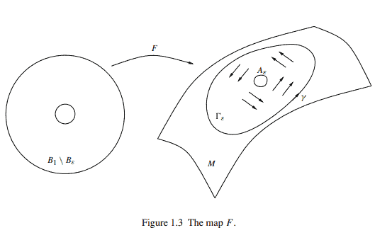
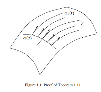
In this section we construct some flows on the one dimensional manifold $Z$. These will be used in following sections to move relative homology cycles. We will take some care in the construction of the flows, to obtain technically useful properties.

Suppose that $g$ is a holomorphic function on $Z$, such as one of the functions $g_{i j}(z)=g_i(z)-g_j(z)$. We want to construct a flow $f(z, t)$ with the property that $f(z, 0)=z$, and $g(f(z, t))$ is “downwind” of $g(z)$ in a certain desired direction. In other words, the time derivative of $g(f(z, t))$ is contained in an angular sector of the form
$$
S(\pm \delta) \stackrel{\text { def }}{=}\left{r e^{i \theta}: \theta \in[\pi-\delta, \pi+\delta]\right}
$$
so $g(f(z, t))$ is contained in an angular sector of the form
$$
S(g(z), \pm \delta) \stackrel{\text { def }}{=}\left{g(z)+r e^{i \theta}: \theta \in[\pi-\delta, \pi+\delta]\right} .
$$
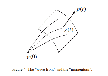
We would also like to insure that at $t=1$, the flow has the effect of moving $g(f(z, t))$ a certain distance away from $g(z)$. This will be possible unless critical points of $g$ are encountered first. We require some special behaviour as the flow moves past critical points. There will be a one dimensional subset $\Lambda \subset \mathrm{C}$, the union of paths which are approximately paths of steepest descent leading away from critical points of $g$. The flow $f$ will have the effect of moving points to $\Lambda$, and then along $\Lambda$ away from the critical points.

Recall that we are admitting the possibility of rotating the $t$ or $\zeta$ planes. This is the same as multiplying the function $g$ by $e^{i \theta}$. After making such a rotation, we can assume that the desired direction of flow is in the negative real direction. Note that $g(P)=0$ for any of the functions $g_{i j}$ considered. Thus rotation preserves $g(P)$.

Our construction of flows will make reference to four numbers, a choice of angular error $\delta$, a choice of small number $\sigma$, a choice of number $L$, and a choice of radius $R$. The number $L$ represents the minimum amount by which the real part of $g$ should be decreased by the flow, unless a critical point is encountered. The angular error represents the maximum allowed deviation from the negative real direction, for the direction in which $g(z)$ moves when $z$ is moved by the flow. The $\sigma$ is a small number which indicates what happens when the flow goes past a critical point.

数学代写|黎曼曲面代写Riemann surface代考|MOVING RELATIVE HOMOLOGY CHAINS

In this section we will describe a formalism for moving relative homology chains. We will form a double complex to calculate relative homology, and then consider homotopies in this complex. It will be done explicitly, so as to facilitate getting bounds.
$Z$ is a complex manifold of dimension one, the universal cover of the original Riemann surface $S$. We consider indices $I=\left(i_0, \ldots, i_n\right)$, saying $|I|=n$. For each such index let $Z_I$ be the space $Z^n$. Let
$$
Z_n=\coprod_{|I|=n} Z_I, \quad Z_*=\coprod_I Z_I .
$$
We will work with chains which are combinations of singular and de Rham chains. Our manifolds will have linear structures, in other words embeddings as open sets in vector spaces. By a $k$-chain on such a manifold $Y$ we will mean a linear functional on the space of $C^{\infty}$ differential $k$-forms on $Y$ which can be expressed as a sum of components of the following form $h(u * H)$. Here $H$ is a $k+l$ dimensional space, compact, with linear structure and algebraic boundary, together with $h: H \rightarrow Y$ a smooth algebraic map (in other words the map is given by coordinate functions which are algebraic over the ring of polynomial functions on $H$ ). It is contracted with a smooth differential $l$-form $u$ on $H$. Such a chain provides a linear functional on the space of $k$-forms $a$ by the rule
$$
\langle h(u * H), a\rangle=\int_H u \wedge h^*(a) .
$$
The reader may think primarily of singular chains (corresponding to the case when $u$ is just the function 1). The more general singular-de Rham chains arise because we use cutoff functions later in the argument. Still, we usually denote $\langle\eta, a\rangle$ by $\int_\eta a$.

These algebraic singular-de Rham chains are functorial with respect to continuous piecewise polynomial maps (even though more general types of currents are not). Suppose $f: Y \rightarrow Y^{\prime}$ is continuous and piecewise polynomial, and suppose $h(u * H)$ is a $k$-chain on $Y$. The composition $f h: H \rightarrow Y^{\prime}$ is continuous and piecewise polynomial. We may further subdivide $H$ into finitely many pieces $H_i$ (with algebraic boundaries) such that on each $H_i, f h$ is polynomial. Let $u_i$ be the restriction of $u$ to $H_i$. Then define
$$
f(h(u * H))=\sum(f h)\left(u_i * H_i\right)
$$

黎曼曲面代考

数学代写|黎曼曲面代写Riemann surface代考|CONSTRUCTION OF FLOWS

在本节中，我们在一维流形上构造一些流 $Z$. 这些将在以下部分中用于移动相对同源循环。我们将在构建 流程时注意一些，以获得技术上有用的属性。
假设 $g$ 是一个全纯函数 $Z$, 比如函数之一 $g_{i j}(z)=g_i(z)-g_j(z)$. 我们要构造一个流 $f(z, t)$ 与财产 $f(z, 0)=z$ ，和 $g(f(z, t))$ 是“顺风”的 $g(z)$ 朝着某个想要的方向。换句话说，时间导数 $g(f(z, t))$ 包含 在表格的角扇区中
所以 $g(f(z, t))$ 包含在表格的角扇区中
我们还想确保在 $t=1$, 流动有移动的效果 $g(f(z, t))$ 距离一定距离 $g(z)$. 这将是可能的，除非关键点 $g$ 最 先遇到。当流经过临界点时，我们需要一些特殊的行为。会有一个一维子集 $\Lambda \subset \mathrm{C}$ ，路径的并集，这些 路径近似于远离临界点的最陡下降路径 $g$. 流量 $f$ 将具有移动点的效果 $\Lambda$, 然后沿着 $\Lambda$ 远离临界点。
回想一下，我们承认旋转的可能性 $t$ 或者 $\zeta$ 飞机。这与乘以函数相同 $g$ 经过 $e^{i \theta}$. 进行这样的旋转后，我们可 以假设所需的流动方向为负实方向。注意 $g(P)=0$ 对于任何功能 $g_{i j}$ 经过考虑的。因此旋转保留 $g(P)$.
我们的流程建设将参考四个数字，角度误差的选择 $\delta$ ，小数的选择 $\sigma$ ，数的选择 $L$ ， 以及半径的选择 $R$. 号码 $L$ 表示实部的最小量 $g$ 应该随流量减少，除非遇到临界点。角度误差表示与负实方向的最大允许偏差，对于 其中的方向 $g(z)$ 移动时 $z$ 被流动所感动。这 $\sigma$ 是一个小数字，表示当流量超过临界点时会发生什么。

数学代写|黎曼曲面代写Riemann surface代考|MOVING RELATIVE HOMOLOGY CHAINS

在本节中，我们将描述移动相对同源链的形式主义。我们将形成一个双复形来计算相对同源性，然后考虑 这个复形中的同伦。它将明确地完成，以便于获得界限。
$Z$ 是一维复流形，原黎曼曲面的普覆盖 $S$. 我们考虑指数 $I=\left(i_0, \ldots, i_n\right)$ ，说 $|I|=n$. 对于每个这样的 索引让 $Z_I$ 成为空间 $Z^n$. 让
$$
Z_n=\coprod_{|I|=n} Z_I, \quad Z_*=\coprod_I Z_I
$$
我们将使用由奇异链和 de Rham 链组合而成的链。我们的流形将具有线性结构，换句话说，嵌入作为向 量空间中的开集。通过一个 $k$-链在这样的流形上 $Y$ 我们将表示空间上的线性泛函 $C^{\infty}$ 微分 $k$-表格 $Y$ 可以表 示为以下形式的组件的总和 $h(u * H)$. 这里 $H$ 是一个 $k+l$ 维空间，紧凑，具有线性结构和代数边界，连 同 $h: H \rightarrow Y$ 光滑的代数映射（换句话说，该映射由坐标函数给出，这些坐标函数是多项式函数环上的 代数函数 $H)$. 它与光滑的微分收缩 $l$-形式 $u$ 在 $H$. 这样的链提供了空间上的线性泛函 $k$-形式 $a$ 按规定
$$
\langle h(u * H), a\rangle=\int_H u \wedge h^*(a) .
$$
读者可能主要想到单数链 (对应于以下情况 $u$ 只是函数 1)。更一般的奇异 de Rham 链的出现是因为我们 在后面的论证中使用了截止函数。尽管如此，我们通常表示 $\langle\eta, a\rangle$ 经过 $\int_\eta a$.
这些代数奇异 de Rham 链是关于连续分段多项式映射的函子 (尽管更一般类型的电流不是)。认为 $f: Y \rightarrow Y^{\prime}$ 是连续的分段多项式，假设 $h(u * H)$ 是一个 $k$-连锁 $Y$. 组成 $f h: H \rightarrow Y^{\prime}$ 是连续的分段多 项式。我们可以进一步细分 $H$ 分成有限多块 $H_i$ （具有代数边界) 使得在每个 $H_i, f h$ 是多项式。让 $u_i$ 是 限制 $u$ 到 $H_i$. 然后定义
$$
f(h(u * H))=\sum(f h)\left(u_i * H_i\right)
$$

统计代写请认准statistics-lab™. statistics-lab™为您的留学生涯保驾护航。

金融工程代写

金融工程是使用数学技术来解决金融问题。金融工程使用计算机科学、统计学、经济学和应用数学领域的工具和知识来解决当前的金融问题，以及设计新的和创新的金融产品。

非参数统计代写

非参数统计指的是一种统计方法，其中不假设数据来自于由少数参数决定的规定模型；这种模型的例子包括正态分布模型和线性回归模型。

广义线性模型代考

广义线性模型（GLM）归属统计学领域，是一种应用灵活的线性回归模型。该模型允许因变量的偏差分布有除了正态分布之外的其它分布。

术语 广义线性模型（GLM）通常是指给定连续和/或分类预测因素的连续响应变量的常规线性回归模型。它包括多元线性回归，以及方差分析和方差分析（仅含固定效应）。

有限元方法代写

有限元方法（FEM）是一种流行的方法，用于数值解决工程和数学建模中出现的微分方程。典型的问题领域包括结构分析、传热、流体流动、质量运输和电磁势等传统领域。

有限元是一种通用的数值方法，用于解决两个或三个空间变量的偏微分方程（即一些边界值问题）。为了解决一个问题，有限元将一个大系统细分为更小、更简单的部分，称为有限元。这是通过在空间维度上的特定空间离散化来实现的，它是通过构建对象的网格来实现的：用于求解的数值域，它有有限数量的点。边界值问题的有限元方法表述最终导致一个代数方程组。该方法在域上对未知函数进行逼近。[1] 然后将模拟这些有限元的简单方程组合成一个更大的方程系统，以模拟整个问题。然后，有限元通过变化微积分使相关的误差函数最小化来逼近一个解决方案。

tatistics-lab作为专业的留学生服务机构，多年来已为美国、英国、加拿大、澳洲等留学热门地的学生提供专业的学术服务，包括但不限于Essay代写，Assignment代写，Dissertation代写，Report代写，小组作业代写，Proposal代写，Paper代写，Presentation代写，计算机作业代写，论文修改和润色，网课代做，exam代考等等。写作范围涵盖高中，本科，研究生等海外留学全阶段，辐射金融，经济学，会计学，审计学，管理学等全球99%专业科目。写作团队既有专业英语母语作者，也有海外名校硕博留学生，每位写作老师都拥有过硬的语言能力，专业的学科背景和学术写作经验。我们承诺100%原创，100%专业，100%准时，100%满意。

随机分析代写

随机微积分是数学的一个分支，对随机过程进行操作。它允许为随机过程的积分定义一个关于随机过程的一致的积分理论。这个领域是由日本数学家伊藤清在第二次世界大战期间创建并开始的。

时间序列分析代写

随机过程，是依赖于参数的一组随机变量的全体，参数通常是时间。 随机变量是随机现象的数量表现，其时间序列是一组按照时间发生先后顺序进行排列的数据点序列。通常一组时间序列的时间间隔为一恒定值（如1秒，5分钟，12小时，7天，1年），因此时间序列可以作为离散时间数据进行分析处理。研究时间序列数据的意义在于现实中，往往需要研究某个事物其随时间发展变化的规律。这就需要通过研究该事物过去发展的历史记录，以得到其自身发展的规律。

回归分析代写

多元回归分析渐进（Multiple Regression Analysis Asymptotics）属于计量经济学领域，主要是一种数学上的统计分析方法，可以分析复杂情况下各影响因素的数学关系，在自然科学、社会和经济学等多个领域内应用广泛。

MATLAB代写

MATLAB 是一种用于技术计算的高性能语言。它将计算、可视化和编程集成在一个易于使用的环境中，其中问题和解决方案以熟悉的数学符号表示。典型用途包括：数学和计算算法开发建模、仿真和原型制作数据分析、探索和可视化科学和工程图形应用程序开发，包括图形用户界面构建MATLAB 是一个交互式系统，其基本数据元素是一个不需要维度的数组。这使您可以解决许多技术计算问题，尤其是那些具有矩阵和向量公式的问题，而只需用 C 或 Fortran 等标量非交互式语言编写程序所需的时间的一小部分。MATLAB 名称代表矩阵实验室。MATLAB 最初的编写目的是提供对由 LINPACK 和 EISPACK 项目开发的矩阵软件的轻松访问，这两个项目共同代表了矩阵计算软件的最新技术。MATLAB 经过多年的发展，得到了许多用户的投入。在大学环境中，它是数学、工程和科学入门和高级课程的标准教学工具。在工业领域，MATLAB 是高效研究、开发和分析的首选工具。MATLAB 具有一系列称为工具箱的特定于应用程序的解决方案。对于大多数 MATLAB 用户来说非常重要，工具箱允许您学习和应用专业技术。工具箱是 MATLAB 函数（M 文件）的综合集合，可扩展 MATLAB 环境以解决特定类别的问题。可用工具箱的领域包括信号处理、控制系统、神经网络、模糊逻辑、小波、仿真等。

R语言代写	问卷设计与分析代写
PYTHON代写	回归分析与线性模型代写
MATLAB代写	方差分析与试验设计代写
STATA代写	机器学习/统计学习代写
SPSS代写	计量经济学代写
EVIEWS代写	时间序列分析代写
EXCEL代写	深度学习代写
SQL代写	各种数据建模与可视化代写

如果你也在 怎样代写黎曼曲面Riemann surface这个学科遇到相关的难题，请随时右上角联系我们的24/7代写客服。

黎曼曲面是一个类似于曲面的构型，它在复平面上覆盖着几个，一般来说是无限多的 “片”。这些薄片可以有非常复杂的结构和相互的联系。

statistics-lab™ 为您的留学生涯保驾护航 在代写黎曼曲面Riemann surface方面已经树立了自己的口碑, 保证靠谱, 高质且原创的统计Statistics代写服务。我们的专家在代写黎曼曲面Riemann surface代写方面经验极为丰富，各种代写黎曼曲面Riemann surface相关的作业也就用不着说。

我们提供的黎曼曲面Riemann surface及其相关学科的代写，服务范围广, 其中包括但不限于:

• Statistical Inference 统计推断
• Statistical Computing 统计计算
• Advanced Probability Theory 高等概率论
• Advanced Mathematical Statistics 高等数理统计学
• (Generalized) Linear Models 广义线性模型
• Statistical Machine Learning 统计机器学习
• Longitudinal Data Analysis 纵向数据分析
• Foundations of Data Science 数据科学基础

数学代写|黎曼曲面代写Riemann surface代考|ORDINARY DIFFERENTIAL EQUATIONS ON A PdEMANN SURFACE

Let $S$ be a compact Riemann surface. We will consider systems of first order ordinary differential equations on $S$
$$
(d-t A-B) m=0
$$
where $A$ and $B$ are $k \times k$ matrices of holomorphic one-forms on $S, t$ is a complex parameter, and $m$ is a column vector or $k \times k$ matrix of functions. We make the following assumption:
$A$ is a diagonal matrix with one-forms $a_1, \ldots, a_k$ along the diagonal. The diagonal entries of $B$ are equal to zero.

The solutions of the system of differential equations are multivalued holomorphic functions on $S$, so it is more convenient to introduce the universal cover $Z=\tilde{S}$. This is complex analytically equivalent to a domain in the complex plane, and it is sometimes useful to keep such an embedding in mind.

Fix a base point $P$ in $Z$ (lying above a base point which we also denote by $P$ in $S$ ). There is a unique matrix valued solution $m(z)$ defined for $z \in Z$, specified by initial conditions $m(P)=I$. For any point $Q$ on $Z$, the value $m(Q)$ is well defined. It depends on the parameter $t$, so we obtain an entire matrix valued function $m(t)=m(Q, t)$ of the complex variable $t$.

Our aim is to investigate the behavior of $m(t)$ as $t \rightarrow \infty$. We can state a theorem which is essentially the main result. Restrict to positive real values of t. Recall that an asymptotic expansion for $m(t)$ is an expression
$$
m(t) \sim \sum_{i=1}^{\Gamma} \sum_{j=J}^{\infty} \sum_{k=0}^{K(j)} c_{i j k} e^{\lambda_i t} t^{-\frac{1}{N}}(\log t)^k
$$
where the real parts of the exponents are equal-say $\Re \lambda_i=\xi$ for all $i$, such that for each $M$ there is a $y(M)$ and a constant $C(M)$ such that for $t \geq y(M)$,
$$
\left|m(t)-\sum_{i=1}^r \sum_{j=J}^{N M} \sum_{k=0}^{K(j)} c_{i j k} e^{\lambda, t} t^{-\frac{1}{N}}(\log t)^k\right| \leq C(M) e^{\xi t} t^{-M} .
$$
Call the numbers $\lambda_i$ the complex exponents of the expansion, and the number $\xi$ the real exponent or just the exponent.

数学代写|黎曼曲面代写Riemann surface代考|LAPLACE TRANSFORM, ASYMPTOTIC EXPANSIONS

Classically, the method of the stationary phase (or steepest descent) provided asymptotic expansions for integrals such as
$$
\int f(z) e^{-t x^2} d z .
$$
In this paper we are interested in obtaining asymptotic expansions for more general integrals such as
$$
m(t)=\int_\eta b e^{t g},
$$
where $g$ is a holomorphic function on a complex manifold, $b$ is a holomorphic differential form of top degree, and $\eta$ is a cycle in homology or relative homology (of real dimension equal to the complex dimension of the manifold). Instead of applying the method of stationary phase directly to such an integral, it will be more useful to take the Laplace transform first. The Laplace transform keeps lower order information which is lost upon going to the asymptotic expansion. If several such integrals are added together and their asymptotic expansions cancel, then an asymptotic expansion at lower exponent can be recovered from the sum of the Laplace transforms.

Suppose that $m(t)$ is an entire holomorphic function of order $\leq 1$. This means that there is a bound
$$
|m(t)| \leq C e^{a|t|} .
$$
The Laplace transform of $m$ is defined to be the integral
$$
f(\zeta)=\int_0^{\infty} m(t) e^{-\zeta t} d t .
$$
The integration is taken along a direction in which the integrand is rapidly decreasing. $f(\zeta)$ is defined and holomorphic for $|\zeta|>a$, and it vanishes at $\infty$. Conversely the function $m(t)$ can be recovered as the inverse Laplace transform
$$
m(t)=\frac{1}{2 \pi i} \oint f(\zeta) e^{\zeta t} d \zeta .
$$
Here the path of integration is a large circle running once counterclockwise around the annulus $|\zeta|>a$.

黎曼曲面代考

数学代写|黎曼曲面代写Riemann surface代考|ORDINARY DIFFERENTIAL EQUATIONS ON A PdEMANN SURFACE

让 $S$ 是一个紧致的黎曼曲面。我们将考虑一阶常微分方程组 $S$
$$
(d-t A-B) m=0
$$
在哪里 $A$ 和 $B$ 是 $k \times k$ 上的全纯单形矩阵 $S, t$ 是一个复杂的参数，并且 $m$ 是列向量或 $k \times k$ 函数矩阵。我 们做出以下假设:
$A$ 是具有一种形式的对角矩阵 $a_1, \ldots, a_k$ 沿着对角线。的对角线条目 $B$ 等于零。
微分方程组的解是上的多值全纯函数 $S$ ，所以引入万能盖更方便 $Z=\tilde{S}$. 这在复杂的分析上等同于复平面 中的域，有时记住这样的嵌入是有用的。
确定一个基点 $P$ 在 $Z$ (位于一个基点之上，我们也用 $P$ 在 $S$ ). 存在唯一矩阵值解 $m(z)$ 定义为 $z \in Z$ ，由初 始条件指定 $m(P)=I$. 对于任何一点 $Q$ 在 $Z$ ， 价值 $m(Q)$ 定义明确。这取决于参数 $t$ ，所以我们得到一个 完整的矩阵值函数 $m(t)=m(Q, t)$ 复杂变量的 $t$.
我们的目标是调查以下行为 $m(t)$ 作为 $t \rightarrow \infty$. 我们可以陈述一个本质上是主要结果的定理。限制为 $\mathrm{t}$ 的 正实数值。回想一下渐近展开 $m(t)$ 是一个表达式
$$
m(t) \sim \sum_{i=1}^{\Gamma} \sum_{j=J}^{\infty} \sum_{k=0}^{K(j)} c_{i j k} e^{\lambda_i t} t^{-\frac{1}{N}}(\log t)^k
$$
指数的实部相等的地方 $\Re \lambda_i=\xi$ 对所有人 $i$ ， 这样对于每个 $M$ 有一个 $y(M)$ 和一个常数 $C(M)$ 这样对于 $t \geq y(M)$
$$
\left|m(t)-\sum_{i=1}^r \sum_{j=J}^{N M} \sum_{k=0}^{K(j)} c_{i j k} e^{\lambda, t} t^{-\frac{1}{N}}(\log t)^k\right| \leq C(M) e^{\xi t} t^{-M}
$$
拨打号码 $\lambda_i$ 展开的复指数和数 $\xi$ 实指数或只是指数。

数学代写|黎曼曲面代写Riemann surface代考|LAPLACE TRANSFORM, ASYMPTOTIC EXPANSIONS

经典地，固定阶段（或最速下降) 的方法为积分提供了渐近展开，例如
$$
\int f(z) e^{-t x^2} d z
$$
在本文中，我们感兴趣的是获得更一般积分的渐近展开，例如
$$
m(t)=\int_\eta b e^{t g},
$$
在哪里 $g$ 是复流形上的全纯函数， $b$ 是最高阶的全纯微分形式，并且 $\eta$ 是同源或相对同源的循环（实维等于 流形的复维)。与其将固定相法直接应用于此类积分，不如先进行拉普拉斯变换更有用。拉普拉斯变换保 留了在进行渐近展开时丢失的低阶信息。如果将几个这样的积分加在一起并且它们的渐近展开抵消，则可 以从拉普拉斯变换的和中恢复较低指数的渐近展开。
假设 $m(t)$ 是阶的整全纯函数 $\leq 1$. 这意味着有界
$$
|m(t)| \leq C e^{a|t|} .
$$
的拉普拉斯变换 $m$ 被定义为积分
$$
f(\zeta)=\int_0^{\infty} m(t) e^{-\zeta t} d t
$$
沿着被积函数快速减小的方向进行积分。 $f(\zeta)$ 被定义并且是全纯的 $|\zeta|>a$ ，它消失在 $\infty$. 函数反之 $m(t)$ 可以恢复为拉普拉斯逆变换
$$
m(t)=\frac{1}{2 \pi i} \oint f(\zeta) e^{\zeta t} d \zeta .
$$
这里积分的路径是一个大圆圈，绕着圆环逆时针方向运行一次 $|\zeta|>a$.

统计代写请认准statistics-lab™. statistics-lab™为您的留学生涯保驾护航。

金融工程代写

金融工程是使用数学技术来解决金融问题。金融工程使用计算机科学、统计学、经济学和应用数学领域的工具和知识来解决当前的金融问题，以及设计新的和创新的金融产品。

非参数统计代写

非参数统计指的是一种统计方法，其中不假设数据来自于由少数参数决定的规定模型；这种模型的例子包括正态分布模型和线性回归模型。

广义线性模型代考

广义线性模型（GLM）归属统计学领域，是一种应用灵活的线性回归模型。该模型允许因变量的偏差分布有除了正态分布之外的其它分布。

术语 广义线性模型（GLM）通常是指给定连续和/或分类预测因素的连续响应变量的常规线性回归模型。它包括多元线性回归，以及方差分析和方差分析（仅含固定效应）。

有限元方法代写

有限元方法（FEM）是一种流行的方法，用于数值解决工程和数学建模中出现的微分方程。典型的问题领域包括结构分析、传热、流体流动、质量运输和电磁势等传统领域。

有限元是一种通用的数值方法，用于解决两个或三个空间变量的偏微分方程（即一些边界值问题）。为了解决一个问题，有限元将一个大系统细分为更小、更简单的部分，称为有限元。这是通过在空间维度上的特定空间离散化来实现的，它是通过构建对象的网格来实现的：用于求解的数值域，它有有限数量的点。边界值问题的有限元方法表述最终导致一个代数方程组。该方法在域上对未知函数进行逼近。[1] 然后将模拟这些有限元的简单方程组合成一个更大的方程系统，以模拟整个问题。然后，有限元通过变化微积分使相关的误差函数最小化来逼近一个解决方案。

tatistics-lab作为专业的留学生服务机构，多年来已为美国、英国、加拿大、澳洲等留学热门地的学生提供专业的学术服务，包括但不限于Essay代写，Assignment代写，Dissertation代写，Report代写，小组作业代写，Proposal代写，Paper代写，Presentation代写，计算机作业代写，论文修改和润色，网课代做，exam代考等等。写作范围涵盖高中，本科，研究生等海外留学全阶段，辐射金融，经济学，会计学，审计学，管理学等全球99%专业科目。写作团队既有专业英语母语作者，也有海外名校硕博留学生，每位写作老师都拥有过硬的语言能力，专业的学科背景和学术写作经验。我们承诺100%原创，100%专业，100%准时，100%满意。

随机分析代写

随机微积分是数学的一个分支，对随机过程进行操作。它允许为随机过程的积分定义一个关于随机过程的一致的积分理论。这个领域是由日本数学家伊藤清在第二次世界大战期间创建并开始的。

时间序列分析代写

随机过程，是依赖于参数的一组随机变量的全体，参数通常是时间。 随机变量是随机现象的数量表现，其时间序列是一组按照时间发生先后顺序进行排列的数据点序列。通常一组时间序列的时间间隔为一恒定值（如1秒，5分钟，12小时，7天，1年），因此时间序列可以作为离散时间数据进行分析处理。研究时间序列数据的意义在于现实中，往往需要研究某个事物其随时间发展变化的规律。这就需要通过研究该事物过去发展的历史记录，以得到其自身发展的规律。

回归分析代写

多元回归分析渐进（Multiple Regression Analysis Asymptotics）属于计量经济学领域，主要是一种数学上的统计分析方法，可以分析复杂情况下各影响因素的数学关系，在自然科学、社会和经济学等多个领域内应用广泛。

MATLAB代写

MATLAB 是一种用于技术计算的高性能语言。它将计算、可视化和编程集成在一个易于使用的环境中，其中问题和解决方案以熟悉的数学符号表示。典型用途包括：数学和计算算法开发建模、仿真和原型制作数据分析、探索和可视化科学和工程图形应用程序开发，包括图形用户界面构建MATLAB 是一个交互式系统，其基本数据元素是一个不需要维度的数组。这使您可以解决许多技术计算问题，尤其是那些具有矩阵和向量公式的问题，而只需用 C 或 Fortran 等标量非交互式语言编写程序所需的时间的一小部分。MATLAB 名称代表矩阵实验室。MATLAB 最初的编写目的是提供对由 LINPACK 和 EISPACK 项目开发的矩阵软件的轻松访问，这两个项目共同代表了矩阵计算软件的最新技术。MATLAB 经过多年的发展，得到了许多用户的投入。在大学环境中，它是数学、工程和科学入门和高级课程的标准教学工具。在工业领域，MATLAB 是高效研究、开发和分析的首选工具。MATLAB 具有一系列称为工具箱的特定于应用程序的解决方案。对于大多数 MATLAB 用户来说非常重要，工具箱允许您学习和应用专业技术。工具箱是 MATLAB 函数（M 文件）的综合集合，可扩展 MATLAB 环境以解决特定类别的问题。可用工具箱的领域包括信号处理、控制系统、神经网络、模糊逻辑、小波、仿真等。

R语言代写	问卷设计与分析代写
PYTHON代写	回归分析与线性模型代写
MATLAB代写	方差分析与试验设计代写
STATA代写	机器学习/统计学习代写
SPSS代写	计量经济学代写
EVIEWS代写	时间序列分析代写
EXCEL代写	深度学习代写
SQL代写	各种数据建模与可视化代写

如果你也在 怎样代写黎曼几何Riemannian geometry这个学科遇到相关的难题，请随时右上角联系我们的24/7代写客服。

黎曼几何是研究黎曼流形的微分几何学分支，黎曼流形是具有黎曼公制的光滑流形，即在每一点的切线空间上有一个内积，从一点到另一点平滑变化。

statistics-lab™ 为您的留学生涯保驾护航 在代写黎曼几何Riemannian geometry方面已经树立了自己的口碑, 保证靠谱, 高质且原创的统计Statistics代写服务。我们的专家在代写黎曼几何Riemannian geometry代写方面经验极为丰富，各种代写黎曼几何Riemannian geometry相关的作业也就用不着说。

我们提供的黎曼几何Riemannian geometry及其相关学科的代写，服务范围广, 其中包括但不限于:

• Statistical Inference 统计推断
• Statistical Computing 统计计算
• Advanced Probability Theory 高等概率论
• Advanced Mathematical Statistics 高等数理统计学
• (Generalized) Linear Models 广义线性模型
• Statistical Machine Learning 统计机器学习
• Longitudinal Data Analysis 纵向数据分析
• Foundations of Data Science 数据科学基础

数学代写|黎曼几何代写Riemannian geometry代考|Gauss–Bonnet Theorem: Global Version

Now we state the global version of the Gauss-Bonnet theorem. In other words we want to generalize (1.33) to the case when $\Gamma$ is a region of $M$ that is not necessarily homeomorphic to a disk; see for instance Figure 1.4. As we will find, the result depends on the Euler characteristic $\chi(\Gamma)$ of this region.

In what follows, by a triangulation of $M$ we mean a decomposition of $M$ into curvilinear polygons (see Definition 1.31). Notice that every compact surface admits a triangulation. ${ }^{3}$

Definition $1.34$ Let $M \subset \mathbb{R}^{3}$ be a compact oriented surface with piecewise smooth boundary $\partial M$. Consider a triangulation of $M$. We define the Euler characteristic of $M$ as
$$
\chi(M):=n_{2}-n_{1}+n_{0},
$$
where $n_{i}$ is the number of $i$-dimensional faces in the triangulation.
The Euler characteristic can be defined for every region $\Gamma$ of $M$ in the same way. Here, by a region $\Gamma$ on a surface $M$ we mean a closed domain of the manifold with piecewise smooth boundary.

数学代写|黎曼几何代写Riemannian geometry代考|Consequences of the Gauss–Bonnet Theorems

Definition $1.39$ Let $M, M^{\prime}$ be two surfaces in $\mathbb{R}^{3}$. A smooth map $\phi: \mathbb{R}^{3} \rightarrow$ $\mathbb{R}^{3}$ is called a local isometry between $M$ and $M^{\prime}$ if $\phi(M)=M^{\prime}$ and for every $q \in M$ it satisfies
$$
\langle v \mid w\rangle=\left\langle D_{q} \phi(v) \mid D_{q} \phi(w)\right\rangle, \quad \forall v, w \in T_{q} M .
$$
If, moreover, the map $\phi$ is a bijection then $\phi$ is called a global isometry. Two surfaces $M$ and $M^{\prime}$ are said to be locally isometric (resp. globally isometric) if there exists a local isometry (resp. global isometry) between $M$ and $M^{\prime}$. Notice that the restriction $\phi$ of an isometry of $\mathbb{R}^{3}$ to a surface $M \subset \mathbb{R}^{3}$ always defines a global isometry between $M$ and $M^{\prime}=\phi(M)$.

Formula (1.52) says that a local isometry between two surfaces $M$ and $M^{\prime}$ preserves the angles between tangent vectors and, a fortiori, the lengths of curves and the distances between points.

By Corollary 1.33, thanks to the fact that the angles and the volumes are preserved by isometries, one obtains that the Gaussian curvature is invariant under local isometries, in the following sense.

Theorem $1.40$ (Gauss’ theorema egregium) Let $\phi$ be a local isometry between $M$ and $M^{\prime}$. Then for every $q \in M$ one has $\kappa(q)=\kappa^{\prime}(\phi(q))$, where $\kappa$ (resp. $\kappa^{\prime}$ ) is the Gaussian curvature of $M$ (resp. $M^{\prime}$ ).

This result says that the Gaussian curvature $\kappa$ depends only on the metric structure on $M$ and not on the specific fact that the surface is embedded in $\mathbb{R}^{3}$ with the induced inner product.

黎曼几何代考

数学代写|黎曼几何代写Riemannian geometry代考|Gauss–Bonnet Theorem: Global Version

现在我们陈述高斯-博内定理的全局版本。换句话说，我们想将 (1.33) 推广到以下情况: $\Gamma$ 是一个地区 $M$ 这不一定与 磁盘同胚；参见图 1.4。我们会发现，结果取决于欧拉特性 $\chi(\Gamma)$ 这个地区的。
接下来，通过三角剖分 $M$ 我们的意思是分解 $M$ 成曲线多边形（见定义 1.31) 。请注意，每个紧致曲面都允许进行 三角剖分。
定义 $1.34$ i上 $M \subset \mathbb{R}^{3}$ 是具有分段光滑边界的紧致曲面 $\partial M$. 考虑三角剖分 $M$. 我们定义欧拉特征 $M$ 作为
$$
\chi(M):=n_{2}-n_{1}+n_{0}
$$
在哪里 $n_{i}$ 是数量 $i$ 三角剖分中的维面。
可以为每个区域定义欧拉特征 $\Gamma$ 的 $M$ 以同样的方式。这里，按地区 $\Gamma$ 在一个表面上 $M$ 我们指的是具有分段平滑边界 的流形的封闭域。

数学代写|黎曼几何代写Riemannian geometry代考|Consequences of the Gauss–Bonnet Theorems

定义1.39让 $M, M^{\prime}$ 是两个曲面 $\mathbb{R}^{3}$. 平滑的地图 $\phi: \mathbb{R}^{3} \rightarrow \mathbb{R}^{3}$ 称为局部等距 $M$ 和 $M^{\prime}$ 如果 $\phi(M)=M^{\prime}$ 并且对于每 个 $q \in M$ 它满足
$$
\langle v \mid w\rangle=\left\langle D_{q} \phi(v) \mid D_{q} \phi(w)\right\rangle, \quad \forall v, w \in T_{q} M .
$$
此外，如果地图 $\phi$ 那么是双射 $\phi$ 称为全局等距。两个表面 $M$ 和 $M^{\prime}$ 如果在两者之间存在局部等距 (或全局等距)，则 称其为局部等距（或全球等距) $M$ 和 $M^{\prime}$. 注意限制 $\phi$ 的等距 $\mathbb{R}^{3}$ 到一个表面 $M \subset \mathbb{R}^{3}$ 总是定义一个全局等距 $M$ 和 $M^{\prime}=\phi(M)$
公式 (1.52) 表示两个表面之间的同部等距 $M$ 和 $M^{\prime}$ 保留切向量之间的角度，更重要的是，保留曲线的长度和点之间 的距离。
根据推论 1.33，由于等距保留了角度和体积这一事实，可以得出在局部等距下高斯曲率是不变的，在以下意义上。
定理1.40 (高斯极好的定理) 让 $\phi$ 是之间的局部等距 $M$ 和 $M^{\prime}$. 那么对于每一个 $q \in M$ 个个有 $\kappa(q)=\kappa^{\prime}(\phi(q))$ ， 在哪里 $\kappa$ (分别。 $\kappa^{\prime}$ ) 是高斯曲率 $M$ (分别。 $M^{\prime}$ ).
这个结果表明高斯曲率 $\kappa$ 仅取决于度量结构 $M$ 而不是表面嵌入的具体事实 $\mathbb{R}^{3}$ 与诱导内积。

统计代写请认准statistics-lab™. statistics-lab™为您的留学生涯保驾护航。

金融工程代写

金融工程是使用数学技术来解决金融问题。金融工程使用计算机科学、统计学、经济学和应用数学领域的工具和知识来解决当前的金融问题，以及设计新的和创新的金融产品。

非参数统计代写

非参数统计指的是一种统计方法，其中不假设数据来自于由少数参数决定的规定模型；这种模型的例子包括正态分布模型和线性回归模型。

广义线性模型代考

广义线性模型（GLM）归属统计学领域，是一种应用灵活的线性回归模型。该模型允许因变量的偏差分布有除了正态分布之外的其它分布。

术语 广义线性模型（GLM）通常是指给定连续和/或分类预测因素的连续响应变量的常规线性回归模型。它包括多元线性回归，以及方差分析和方差分析（仅含固定效应）。

有限元方法代写

有限元方法（FEM）是一种流行的方法，用于数值解决工程和数学建模中出现的微分方程。典型的问题领域包括结构分析、传热、流体流动、质量运输和电磁势等传统领域。

有限元是一种通用的数值方法，用于解决两个或三个空间变量的偏微分方程（即一些边界值问题）。为了解决一个问题，有限元将一个大系统细分为更小、更简单的部分，称为有限元。这是通过在空间维度上的特定空间离散化来实现的，它是通过构建对象的网格来实现的：用于求解的数值域，它有有限数量的点。边界值问题的有限元方法表述最终导致一个代数方程组。该方法在域上对未知函数进行逼近。[1] 然后将模拟这些有限元的简单方程组合成一个更大的方程系统，以模拟整个问题。然后，有限元通过变化微积分使相关的误差函数最小化来逼近一个解决方案。

tatistics-lab作为专业的留学生服务机构，多年来已为美国、英国、加拿大、澳洲等留学热门地的学生提供专业的学术服务，包括但不限于Essay代写，Assignment代写，Dissertation代写，Report代写，小组作业代写，Proposal代写，Paper代写，Presentation代写，计算机作业代写，论文修改和润色，网课代做，exam代考等等。写作范围涵盖高中，本科，研究生等海外留学全阶段，辐射金融，经济学，会计学，审计学，管理学等全球99%专业科目。写作团队既有专业英语母语作者，也有海外名校硕博留学生，每位写作老师都拥有过硬的语言能力，专业的学科背景和学术写作经验。我们承诺100%原创，100%专业，100%准时，100%满意。

随机分析代写

随机微积分是数学的一个分支，对随机过程进行操作。它允许为随机过程的积分定义一个关于随机过程的一致的积分理论。这个领域是由日本数学家伊藤清在第二次世界大战期间创建并开始的。

时间序列分析代写

随机过程，是依赖于参数的一组随机变量的全体，参数通常是时间。 随机变量是随机现象的数量表现，其时间序列是一组按照时间发生先后顺序进行排列的数据点序列。通常一组时间序列的时间间隔为一恒定值（如1秒，5分钟，12小时，7天，1年），因此时间序列可以作为离散时间数据进行分析处理。研究时间序列数据的意义在于现实中，往往需要研究某个事物其随时间发展变化的规律。这就需要通过研究该事物过去发展的历史记录，以得到其自身发展的规律。

回归分析代写

多元回归分析渐进（Multiple Regression Analysis Asymptotics）属于计量经济学领域，主要是一种数学上的统计分析方法，可以分析复杂情况下各影响因素的数学关系，在自然科学、社会和经济学等多个领域内应用广泛。

MATLAB代写

MATLAB 是一种用于技术计算的高性能语言。它将计算、可视化和编程集成在一个易于使用的环境中，其中问题和解决方案以熟悉的数学符号表示。典型用途包括：数学和计算算法开发建模、仿真和原型制作数据分析、探索和可视化科学和工程图形应用程序开发，包括图形用户界面构建MATLAB 是一个交互式系统，其基本数据元素是一个不需要维度的数组。这使您可以解决许多技术计算问题，尤其是那些具有矩阵和向量公式的问题，而只需用 C 或 Fortran 等标量非交互式语言编写程序所需的时间的一小部分。MATLAB 名称代表矩阵实验室。MATLAB 最初的编写目的是提供对由 LINPACK 和 EISPACK 项目开发的矩阵软件的轻松访问，这两个项目共同代表了矩阵计算软件的最新技术。MATLAB 经过多年的发展，得到了许多用户的投入。在大学环境中，它是数学、工程和科学入门和高级课程的标准教学工具。在工业领域，MATLAB 是高效研究、开发和分析的首选工具。MATLAB 具有一系列称为工具箱的特定于应用程序的解决方案。对于大多数 MATLAB 用户来说非常重要，工具箱允许您学习和应用专业技术。工具箱是 MATLAB 函数（M 文件）的综合集合，可扩展 MATLAB 环境以解决特定类别的问题。可用工具箱的领域包括信号处理、控制系统、神经网络、模糊逻辑、小波、仿真等。

R语言代写	问卷设计与分析代写
PYTHON代写	回归分析与线性模型代写
MATLAB代写	方差分析与试验设计代写
STATA代写	机器学习/统计学习代写
SPSS代写	计量经济学代写
EVIEWS代写	时间序列分析代写
EXCEL代写	深度学习代写
SQL代写	各种数据建模与可视化代写

如果你也在 怎样代写黎曼几何Riemannian geometry这个学科遇到相关的难题，请随时右上角联系我们的24/7代写客服。

黎曼几何是研究黎曼流形的微分几何学分支，黎曼流形是具有黎曼公制的光滑流形，即在每一点的切线空间上有一个内积，从一点到另一点平滑变化。

statistics-lab™ 为您的留学生涯保驾护航 在代写黎曼几何Riemannian geometry方面已经树立了自己的口碑, 保证靠谱, 高质且原创的统计Statistics代写服务。我们的专家在代写黎曼几何Riemannian geometry代写方面经验极为丰富，各种代写黎曼几何Riemannian geometry相关的作业也就用不着说。

我们提供的黎曼几何Riemannian geometry及其相关学科的代写，服务范围广, 其中包括但不限于:

• Statistical Inference 统计推断
• Statistical Computing 统计计算
• Advanced Probability Theory 高等概率论
• Advanced Mathematical Statistics 高等数理统计学
• (Generalized) Linear Models 广义线性模型
• Statistical Machine Learning 统计机器学习
• Longitudinal Data Analysis 纵向数据分析
• Foundations of Data Science 数据科学基础

数学代写|黎曼几何代写Riemannian geometry代考|Gauss–Bonnet Theorems

In this section we will prove both the local and the global version of the GaussBonnet theorem. A strong consequence of these results is the celebrated Gauss’ theorema egregium, which says that the Gaussian curvature of a surface is independent of its embedding in $\mathbb{R}^{3}$.

Definition $1.29$ Let $\gamma:[0, T] \rightarrow M$ be a smooth curve parametrized by arclength. The geodesic curvature of $\gamma$ is defined as
$$
\rho_{\gamma}(t)=\omega_{\dot{\gamma}(t)}(\ddot{\gamma}(t))
$$
Nótice that if $\gamma$ is a géodésic, thên $\rho_{\gamma}(t)=0$ fố everry $t \in[0, T]$. Thé geodesic curvature measures how far a curve is from being a geodesic.

Remark $1.30$ The geodesic curvature changes sign if we move along the curve in the opposite direction. Moreover, if $M=\mathbb{R}^{2}$, it coincides with the usual notion of the curvature of a planar curve.

数学代写|黎曼几何代写Riemannian geometry代考|Gauss–Bonnet Theorem: Local Version

A regular polygon in $\mathbb{R}^{2}$ is a polygon that is equiangular and equilateral. We include disks among regular polygons (as a limiting case, when the number of edges is infinite).

Definition 1.31 A curvilinear polygon $\Gamma$ on an oriented surface $M$ is the image of a regular polygon in $\mathbb{R}^{2}$ under a diffeomorphism. We assume that $\partial \Gamma$ is oriented consistently with the orientation of $M$.

Notice that a curvilinear polygon is always homeomorphic to a disk, and the case when $\partial \Gamma$ is smooth (and $\Gamma$ is diffeomorphic to the disk) is included in the definition.

In what follows, given a curvilinear polygon $\Gamma$ on an oriented surface $M$ (see Figure 1.2), we denote by

• $\gamma_{i}: I_{i} \rightarrow M$, for $i=1, \ldots, m$, the smooth curves parametrized by arc length, with orientation consistent with $\partial \Gamma$, such that $\partial \Gamma=\cup_{i=1}^{m} \gamma_{i}\left(I_{i}\right)$,
• $\alpha_{i}$, for $i=1, \ldots, m$, the external angles at the points where $\partial \Gamma$ is not $C^{1}$.
  Theorem 1.32 (Gauss-Bonnet, local version) Let $\Gamma$ be a curvilinear polygon on an oriented surface $M$. Then we have
  $$
  \int_{\Gamma} \kappa d V+\sum_{i=1}^{m} \int_{I_{i}} \rho_{\gamma_{i}}(t) d t+\sum_{i=1}^{m} \alpha_{i}=2 \pi
  $$
  Proof (a) The case where $\partial \Gamma$ is smooth. In this case $\Gamma$ is the image of the unit (closed) ball $B_{1}$, centered at the origin of $\mathbb{R}^{2}$, under a diffeomorphism
  $$
  F: B_{1} \rightarrow M . \quad \Gamma=F\left(B_{1}\right) .
  $$
  In what follows we denote by $\gamma: I \rightarrow M$ the curve such that $\gamma(I)=\partial \Gamma$. We consider on $B_{1}$ the vector field $V(x)=x_{1} \partial_{x_{2}}-x_{2} \partial_{x_{1}}$ which has an isolated zero at the origin and whose flow is a rotation around zero. Denote by $X:=F_{*} V$ the induced vector field on $M$ with critical point $q_{0}=F(0)$.

黎曼几何代考

数学代写|黎曼几何代写Riemannian geometry代考|Gauss–Bonnet Theorems

在本节中，我们将证明 GaussBonnet 定理的局部和全局版本。这些结果的一个重要结果是苃名的高斯偏偏定理，它 说表面的高斯曲率与其嵌入 $\mathbb{R}^{3}$.
定义 $1.29$ 让 $\gamma:[0, T] \rightarrow M$ 是由弧长参数化的平滑曲线。的测地曲率 $\gamma$ 定义为
$$
\rho_{\gamma}(t)=\omega_{\dot{\gamma}(t)}(\ddot{\gamma}(t))
$$
请注意，如果 $\gamma$ 是测地线，那么 $\rho_{\gamma}(t)=0$ ố 每一个 $t \in[0, T]$. 测地线曲率测量曲线与测地线之间的距离。
评论 $1.30$ 如果我们沿相反方向的曲线移动，测地线曲率会改变符号。此外，如果 $M=\mathbb{R}^{2}$ ，它与平面曲线曲率的通常概念一致。

数学代写|黎曼几何代写Riemannian geometry代考|Gauss–Bonnet Theorem: Local Version

一个正多边形 $\mathbb{R}^{2}$ 是等角和等边的多边形。我们在正多边形中包含圆盘（作为限制情况，当边数是无限时）。
定义 $1.31$ 曲线多边形 $\Gamma$ 在定向表面上 $M$ 是正多边形的图像 $\mathbb{R}^{2}$ 在微分同胚之下。我们假设 $\partial \Gamma$ 与方向一致 $M$.
请注意，曲线多边形始终与圆盘同胚，并且当 $\partial \Gamma$ 是光滑的（并且 $\Gamma$ 与圆盘微分同胚) 包含在定义中。
下面，给定一个曲线多边形 $\Gamma$ 在定向表面上 $M$ （见图 1.2），我们用

• $\gamma_{i}: I_{i} \rightarrow M$ ，为了 $i=1, \ldots, m$, 由弧长参数化的平滑曲线，方向与 $\partial \Gamma$, 这样 $\partial \Gamma=\cup_{i=1}^{m} \gamma_{i}\left(I_{i}\right)$,
  定理 $1.32$ (Gauss-Bonnet，本地版本) 让 $\Gamma$ 是有向曲面上的曲线多边形 $M$. 然后我们有
  $$
  \int_{\Gamma} \kappa d V+\sum_{i=1}^{m} \int_{I_{i}} \rho_{\gamma_{i}}(t) d t+\sum_{i=1}^{m} \alpha_{i}=2 \pi
  $$
  证明 (a) 情况 $\partial \Gamma$ 是光滑的。在这种情况下 $\Gamma$ 是单位（封闭) 球的形象 $B_{1}$ ，以原点为中心 $\mathbb{R}^{2}$ ，在微分同胚下
  $$
  F: B_{1} \rightarrow M . \quad \Gamma=F\left(B_{1}\right) .
  $$
  下面我们用 $\gamma: I \rightarrow M$ 曲线使得 $\gamma(I)=\partial \Gamma$. 我们考虑 $B_{1}$ 向量场 $V(x)=x_{1} \partial_{x_{2}}-x_{2} \partial_{x_{1}}$ 它在原点有一个 孤立的零，其流动是围绕零旋转。表示为 $X:=F_{*} V$ 上的诱导矢量场 $M$ 有临界点 $q_{0}=F(0)$.

统计代写请认准statistics-lab™. statistics-lab™为您的留学生涯保驾护航。

金融工程代写

金融工程是使用数学技术来解决金融问题。金融工程使用计算机科学、统计学、经济学和应用数学领域的工具和知识来解决当前的金融问题，以及设计新的和创新的金融产品。

非参数统计代写

非参数统计指的是一种统计方法，其中不假设数据来自于由少数参数决定的规定模型；这种模型的例子包括正态分布模型和线性回归模型。

广义线性模型代考

广义线性模型（GLM）归属统计学领域，是一种应用灵活的线性回归模型。该模型允许因变量的偏差分布有除了正态分布之外的其它分布。

术语 广义线性模型（GLM）通常是指给定连续和/或分类预测因素的连续响应变量的常规线性回归模型。它包括多元线性回归，以及方差分析和方差分析（仅含固定效应）。

有限元方法代写

有限元方法（FEM）是一种流行的方法，用于数值解决工程和数学建模中出现的微分方程。典型的问题领域包括结构分析、传热、流体流动、质量运输和电磁势等传统领域。

有限元是一种通用的数值方法，用于解决两个或三个空间变量的偏微分方程（即一些边界值问题）。为了解决一个问题，有限元将一个大系统细分为更小、更简单的部分，称为有限元。这是通过在空间维度上的特定空间离散化来实现的，它是通过构建对象的网格来实现的：用于求解的数值域，它有有限数量的点。边界值问题的有限元方法表述最终导致一个代数方程组。该方法在域上对未知函数进行逼近。[1] 然后将模拟这些有限元的简单方程组合成一个更大的方程系统，以模拟整个问题。然后，有限元通过变化微积分使相关的误差函数最小化来逼近一个解决方案。

tatistics-lab作为专业的留学生服务机构，多年来已为美国、英国、加拿大、澳洲等留学热门地的学生提供专业的学术服务，包括但不限于Essay代写，Assignment代写，Dissertation代写，Report代写，小组作业代写，Proposal代写，Paper代写，Presentation代写，计算机作业代写，论文修改和润色，网课代做，exam代考等等。写作范围涵盖高中，本科，研究生等海外留学全阶段，辐射金融，经济学，会计学，审计学，管理学等全球99%专业科目。写作团队既有专业英语母语作者，也有海外名校硕博留学生，每位写作老师都拥有过硬的语言能力，专业的学科背景和学术写作经验。我们承诺100%原创，100%专业，100%准时，100%满意。

随机分析代写

随机微积分是数学的一个分支，对随机过程进行操作。它允许为随机过程的积分定义一个关于随机过程的一致的积分理论。这个领域是由日本数学家伊藤清在第二次世界大战期间创建并开始的。

时间序列分析代写

随机过程，是依赖于参数的一组随机变量的全体，参数通常是时间。 随机变量是随机现象的数量表现，其时间序列是一组按照时间发生先后顺序进行排列的数据点序列。通常一组时间序列的时间间隔为一恒定值（如1秒，5分钟，12小时，7天，1年），因此时间序列可以作为离散时间数据进行分析处理。研究时间序列数据的意义在于现实中，往往需要研究某个事物其随时间发展变化的规律。这就需要通过研究该事物过去发展的历史记录，以得到其自身发展的规律。

回归分析代写

多元回归分析渐进（Multiple Regression Analysis Asymptotics）属于计量经济学领域，主要是一种数学上的统计分析方法，可以分析复杂情况下各影响因素的数学关系，在自然科学、社会和经济学等多个领域内应用广泛。

MATLAB代写

MATLAB 是一种用于技术计算的高性能语言。它将计算、可视化和编程集成在一个易于使用的环境中，其中问题和解决方案以熟悉的数学符号表示。典型用途包括：数学和计算算法开发建模、仿真和原型制作数据分析、探索和可视化科学和工程图形应用程序开发，包括图形用户界面构建MATLAB 是一个交互式系统，其基本数据元素是一个不需要维度的数组。这使您可以解决许多技术计算问题，尤其是那些具有矩阵和向量公式的问题，而只需用 C 或 Fortran 等标量非交互式语言编写程序所需的时间的一小部分。MATLAB 名称代表矩阵实验室。MATLAB 最初的编写目的是提供对由 LINPACK 和 EISPACK 项目开发的矩阵软件的轻松访问，这两个项目共同代表了矩阵计算软件的最新技术。MATLAB 经过多年的发展，得到了许多用户的投入。在大学环境中，它是数学、工程和科学入门和高级课程的标准教学工具。在工业领域，MATLAB 是高效研究、开发和分析的首选工具。MATLAB 具有一系列称为工具箱的特定于应用程序的解决方案。对于大多数 MATLAB 用户来说非常重要，工具箱允许您学习和应用专业技术。工具箱是 MATLAB 函数（M 文件）的综合集合，可扩展 MATLAB 环境以解决特定类别的问题。可用工具箱的领域包括信号处理、控制系统、神经网络、模糊逻辑、小波、仿真等。

R语言代写	问卷设计与分析代写
PYTHON代写	回归分析与线性模型代写
MATLAB代写	方差分析与试验设计代写
STATA代写	机器学习/统计学习代写
SPSS代写	计量经济学代写
EVIEWS代写	时间序列分析代写
EXCEL代写	深度学习代写
SQL代写	各种数据建模与可视化代写

如果你也在 怎样代写黎曼几何Riemannian geometry这个学科遇到相关的难题，请随时右上角联系我们的24/7代写客服。

黎曼几何是研究黎曼流形的微分几何学分支，黎曼流形是具有黎曼公制的光滑流形，即在每一点的切线空间上有一个内积，从一点到另一点平滑变化。

statistics-lab™ 为您的留学生涯保驾护航 在代写黎曼几何Riemannian geometry方面已经树立了自己的口碑, 保证靠谱, 高质且原创的统计Statistics代写服务。我们的专家在代写黎曼几何Riemannian geometry代写方面经验极为丰富，各种代写黎曼几何Riemannian geometry相关的作业也就用不着说。

我们提供的黎曼几何Riemannian geometry及其相关学科的代写，服务范围广, 其中包括但不限于:

• Statistical Inference 统计推断
• Statistical Computing 统计计算
• Advanced Probability Theory 高等概率论
• Advanced Mathematical Statistics 高等数理统计学
• (Generalized) Linear Models 广义线性模型
• Statistical Machine Learning 统计机器学习
• Longitudinal Data Analysis 纵向数据分析
• Foundations of Data Science 数据科学基础

数学代写|黎曼几何代写Riemannian geometry代考|Parallel Transport

In this section we want to introduce the notion of parallel transport on a surface (along a curve), which allows us to define its main geometric invariant: the Gaussian curvature.

Definition $1.14$ Let $\gamma:[0, T] \rightarrow M$ be a smooth curve. A smooth curve of tangent vectors $\xi(t) \in T_{\nu(t)} M$ is said to be parallel if $\dot{\xi}(t) \perp T_{\gamma(t)} M$.

This notion generalizes the notion of parallelism of vectors on the plane, where it is possible to canonically identify every tangent space to $M=\mathbb{R}^{2}$ with $\mathbb{R}^{2}$ itself. ${ }^{2}$ In this case a smooth curve of tangent vectors $\xi(t) \in T_{\gamma(t)} M$ is parallel if and only if $\dot{\xi}(t)=0$.

When $M$ is the zero level of a smooth function $a: \mathbb{R}^{3} \rightarrow \mathbb{R}$, as in (1.14), we have the following description:

Proposition $1.15$ A smooth curve of tangent vectors $\xi(t)$ defined along $\gamma:[0, T] \rightarrow M$ is parallel if and only if it satisfies
$$
\dot{\xi}(t)=-\frac{\dot{\gamma}(t)^{T}\left(\nabla_{\gamma(t)}^{2} a\right) \xi(t)}{\left|\nabla_{\gamma(t)} a\right|^{2}} \nabla_{\gamma(t)} a, \quad \forall t \in[0, T] .
$$
Proof As in Remark 1.7, $\xi(t) \in T_{\gamma(t)} M$ implies that $\left\langle\nabla_{\gamma(t)} a, \xi(t)\right\rangle=0$. Moreover, by assumption, $\dot{\xi}(t)=\alpha(t) \nabla_{\gamma(t)} a$ for some smooth function $\alpha$. With computations analogous to those in the proof of Proposition $1.8$ we get that
$$
\dot{\gamma}(t)^{T}\left(\nabla_{\gamma(t)}^{2} a\right) \xi(t)+\alpha(t)\left|\nabla_{\gamma(t)} a\right|^{2}=0,
$$
from which the statement follows.

数学代写|黎曼几何代写Riemannian geometry代考|Parallel Transport and the Levi-Civita Connection

Definition 1.19 An orientation of a surface $M$ is a smooth map $v: M \rightarrow \mathbb{R}^{3}$, défineed globally on $M$, such that $v(q) \perp T_{q} M$ and $|v(q)|=1$ for every $q \in M$. Notice that if $v$ is an orientation of $M$, then $-v$ also defines an orientation of $M$.

A surface $M$ is oriented if it is given (when this exists) an orientation. On an oriented surface $M$, an orthonormal frame $\left{e_{1}, e_{2}\right}$ of $T_{q} M$ is said to be positively oriented (resp. negatively oriented) if $e_{1} \wedge e_{2}=k v(q)$ with $k>0$ (resp. $k<0$ ).
In the following we assume that $M$ is an oriented surface.
Definition $1.20$ The spherical bundle $S M$ on $M$ is the disjoint union of all unit tangent vectors to $M$ :
$$
S M=\bigsqcup_{q \in M} S_{q} M, \quad S_{q} M=\left{v \in T_{q} M,|v|=1\right}
$$
The spherical bundle $S M$ can be endowed with the structure of a smooth manifold of dimension 3 , and more precisely of a fiber bundle with base manifold $M$, typical fiber $S^{1}$ and canonical projection
$$
\pi: S M \rightarrow M, \quad \pi(v)=q \quad \text { if } v \in T_{q} M
$$

Remark $1.21$ Fix a positively oriented local orthonormal frame $\left{e_{1}(q), e_{2}(q)\right}$ on $M$. Since every vector in the fiber $S_{q} M$ has norm 1, we can write every $v \in S_{q} M$ as $v=(\cos \theta) e_{1}(q)+(\sin \theta) e_{2}(q)$ for $\theta \in S^{1}$.

The choice of such an orthonormal frame then induces coordinates $(q, \theta)$ on $S M$. Notice that the choice of a different positively oriented local orthonormal frame $\left{e_{1}^{\prime}(q), e_{2}^{\prime}(q)\right}$ induces coordinates $\left(q^{\prime}, \theta^{\prime}\right)$ on $S M$, where $q^{\prime}=q$ and $\theta^{\prime}=\theta+\phi(q)$ for $\phi \in C^{\infty}(M)$

The orientation of $M$ permits us, once a unit tangent vector is given, to define a canonical orthonormal frame.

黎曼几何代考

数学代写|黎曼几何代写Riemannian geometry代考|Parallel Transport

在本节中，我们要介绍表面 (沿曲线) 上的平行传输的概念，它允许我们定义其主要的几何不变量: 高斯曲率。
定义1.14让 $\gamma:[0, T] \rightarrow M$ 成为一条平滑的曲线。切向量的平滑曲线 $\xi(t) \in T_{\nu(t)} M$ 据说是平行的，如果 $\dot{\xi}(t) \perp T_{\gamma(t)} M$.
这个概念概括了平面上向量平行度的概念，其中可以规范地识别每个切线空间 $M=\mathbb{R}^{2}$ 和 $\mathbb{R}^{2}$ 本身。 ${ }^{2}$ 在这种情况 下，切向量的平滑曲线 $\xi(t) \in T_{\gamma(t)} M$ 当且仅当是平行的 $\dot{\xi}(t)=0$.
什么时候 $M$ 是平滑函数的零水平 $a: \mathbb{R}^{3} \rightarrow \mathbb{R}$ ，如（1.14）中，我们有以下描述：
主张 $1.15$ 切向量的平滑曲线 $\xi(t)$ 沿定义 $\gamma:[0, T] \rightarrow M$ 当且仅当它满足时是平行的
$$
\dot{\xi}(t)=-\frac{\dot{\gamma}(t)^{T}\left(\nabla_{\gamma(t)}^{2} a\right) \xi(t)}{\left|\nabla_{\gamma(t)} a\right|^{2}} \nabla_{\gamma(t)} a, \quad \forall t \in[0, T] .
$$
证明 如备注 1.7， $\xi(t) \in T_{\gamma(t)} M$ 暗示 $\left\langle\nabla_{\gamma(t)} a, \xi(t)\right\rangle=0$. 此外，根据假设， $\dot{\xi}(t)=\alpha(t) \nabla_{\gamma(t)} a$ 对于一些平滑 的功能 $\alpha$. 计算类似于命题证明中的计算 $1.8$ 我们明白了
$$
\dot{\gamma}(t)^{T}\left(\nabla_{\gamma(t)}^{2} a\right) \xi(t)+\alpha(t)\left|\nabla_{\gamma(t)} a\right|^{2}=0,
$$
声明如下。

数学代写|黎曼几何代写Riemannian geometry代考|Parallel Transport and the Levi-Civita Connection

定义 $1.19$ 表面的方向 $M$ 是一张光滑的地图 $v: M \rightarrow \mathbb{R}^{3}$ ，全局定义在 $M$, 这样 $v(q) \perp T_{q} M$ 和 $|v(q)|=1$ 对于每 个 $q \in M$. 请注意，如果 $v$ 是一个方向 $M$ ，然后 $-v$ 还定义了一个方向 $M$.
一个表面 $M$ 如果给定 (如果存在) 一个方向，则它是有方向的。在定向表面上 $M ， 一 个$ 个正交框架
Uleft{e_{1}, e_{2} \right } } \text { 的 } T _ { q } M \text { 如果 } e _ { 1 } \wedge e _ { 2 } = k v ( q ) \text { 和 } k > 0 \text { (分别。 } k < 0 \text { )。 }
下面我们假设 $M$ 是一个定向曲面。
定义1.20球形束 $S M$ 上 $M$ 是所有单位切向量的不相交并集到 $M$ :
S M=\bigsqcup_{q \in M $} S_{-}{q} M, \backslash q u a d S_{-}{q} M=\backslash \mid e f t\left{v \backslash\right.$ in $T_{-}{q} M,|v|=1 \backslash$ right $}$
球形束 $S M$ 可以被赋予一个维数为 3 的光滑流形的结构，更准确地说是一个带有基流形的纤维束 $M$ ，典型纤维 $S^{1}$ 和
正则投影
$$
\pi: S M \rightarrow M, \quad \pi(v)=q \quad \text { if } v \in T_{q} M
$$
评论1.21修复一个正向的同部正交坐标系 $\$ left{e_{1}(q), e_{2}(q)\right} 上 $M$. 由于光纤中的每个向量 $S_{q} M$ 有范数 1 ， 我们可以写出每个 $v \in S_{q} M$ 作为 $v=(\cos \theta) e_{1}(q)+(\sin \theta) e_{2}(q)$ 为了 $\theta \in S^{1}$.
选择这样一个正交坐标系然后得出坐标 $(q, \theta)$ 上 $S M$. 请注意，选择不同的正向局部正交坐标系 $\phi \in C^{\infty}(M)$
的方向 $M$ 允许我们，一旦给定一个单位切向量，就可以定义一个标准正交坐标系。

统计代写请认准statistics-lab™. statistics-lab™为您的留学生涯保驾护航。

金融工程代写

金融工程是使用数学技术来解决金融问题。金融工程使用计算机科学、统计学、经济学和应用数学领域的工具和知识来解决当前的金融问题，以及设计新的和创新的金融产品。

非参数统计代写

非参数统计指的是一种统计方法，其中不假设数据来自于由少数参数决定的规定模型；这种模型的例子包括正态分布模型和线性回归模型。

广义线性模型代考

广义线性模型（GLM）归属统计学领域，是一种应用灵活的线性回归模型。该模型允许因变量的偏差分布有除了正态分布之外的其它分布。

术语 广义线性模型（GLM）通常是指给定连续和/或分类预测因素的连续响应变量的常规线性回归模型。它包括多元线性回归，以及方差分析和方差分析（仅含固定效应）。

有限元方法代写

有限元方法（FEM）是一种流行的方法，用于数值解决工程和数学建模中出现的微分方程。典型的问题领域包括结构分析、传热、流体流动、质量运输和电磁势等传统领域。

有限元是一种通用的数值方法，用于解决两个或三个空间变量的偏微分方程（即一些边界值问题）。为了解决一个问题，有限元将一个大系统细分为更小、更简单的部分，称为有限元。这是通过在空间维度上的特定空间离散化来实现的，它是通过构建对象的网格来实现的：用于求解的数值域，它有有限数量的点。边界值问题的有限元方法表述最终导致一个代数方程组。该方法在域上对未知函数进行逼近。[1] 然后将模拟这些有限元的简单方程组合成一个更大的方程系统，以模拟整个问题。然后，有限元通过变化微积分使相关的误差函数最小化来逼近一个解决方案。

tatistics-lab作为专业的留学生服务机构，多年来已为美国、英国、加拿大、澳洲等留学热门地的学生提供专业的学术服务，包括但不限于Essay代写，Assignment代写，Dissertation代写，Report代写，小组作业代写，Proposal代写，Paper代写，Presentation代写，计算机作业代写，论文修改和润色，网课代做，exam代考等等。写作范围涵盖高中，本科，研究生等海外留学全阶段，辐射金融，经济学，会计学，审计学，管理学等全球99%专业科目。写作团队既有专业英语母语作者，也有海外名校硕博留学生，每位写作老师都拥有过硬的语言能力，专业的学科背景和学术写作经验。我们承诺100%原创，100%专业，100%准时，100%满意。

随机分析代写

随机微积分是数学的一个分支，对随机过程进行操作。它允许为随机过程的积分定义一个关于随机过程的一致的积分理论。这个领域是由日本数学家伊藤清在第二次世界大战期间创建并开始的。

时间序列分析代写

随机过程，是依赖于参数的一组随机变量的全体，参数通常是时间。 随机变量是随机现象的数量表现，其时间序列是一组按照时间发生先后顺序进行排列的数据点序列。通常一组时间序列的时间间隔为一恒定值（如1秒，5分钟，12小时，7天，1年），因此时间序列可以作为离散时间数据进行分析处理。研究时间序列数据的意义在于现实中，往往需要研究某个事物其随时间发展变化的规律。这就需要通过研究该事物过去发展的历史记录，以得到其自身发展的规律。

回归分析代写

多元回归分析渐进（Multiple Regression Analysis Asymptotics）属于计量经济学领域，主要是一种数学上的统计分析方法，可以分析复杂情况下各影响因素的数学关系，在自然科学、社会和经济学等多个领域内应用广泛。

MATLAB代写

MATLAB 是一种用于技术计算的高性能语言。它将计算、可视化和编程集成在一个易于使用的环境中，其中问题和解决方案以熟悉的数学符号表示。典型用途包括：数学和计算算法开发建模、仿真和原型制作数据分析、探索和可视化科学和工程图形应用程序开发，包括图形用户界面构建MATLAB 是一个交互式系统，其基本数据元素是一个不需要维度的数组。这使您可以解决许多技术计算问题，尤其是那些具有矩阵和向量公式的问题，而只需用 C 或 Fortran 等标量非交互式语言编写程序所需的时间的一小部分。MATLAB 名称代表矩阵实验室。MATLAB 最初的编写目的是提供对由 LINPACK 和 EISPACK 项目开发的矩阵软件的轻松访问，这两个项目共同代表了矩阵计算软件的最新技术。MATLAB 经过多年的发展，得到了许多用户的投入。在大学环境中，它是数学、工程和科学入门和高级课程的标准教学工具。在工业领域，MATLAB 是高效研究、开发和分析的首选工具。MATLAB 具有一系列称为工具箱的特定于应用程序的解决方案。对于大多数 MATLAB 用户来说非常重要，工具箱允许您学习和应用专业技术。工具箱是 MATLAB 函数（M 文件）的综合集合，可扩展 MATLAB 环境以解决特定类别的问题。可用工具箱的领域包括信号处理、控制系统、神经网络、模糊逻辑、小波、仿真等。

R语言代写	问卷设计与分析代写
PYTHON代写	回归分析与线性模型代写
MATLAB代写	方差分析与试验设计代写
STATA代写	机器学习/统计学习代写
SPSS代写	计量经济学代写
EVIEWS代写	时间序列分析代写
EXCEL代写	深度学习代写
SQL代写	各种数据建模与可视化代写

如果你也在 怎样代写黎曼几何Riemannian geometry这个学科遇到相关的难题，请随时右上角联系我们的24/7代写客服。

黎曼几何是研究黎曼流形的微分几何学分支，黎曼流形是具有黎曼公制的光滑流形，即在每一点的切线空间上有一个内积，从一点到另一点平滑变化。

statistics-lab™ 为您的留学生涯保驾护航 在代写黎曼几何Riemannian geometry方面已经树立了自己的口碑, 保证靠谱, 高质且原创的统计Statistics代写服务。我们的专家在代写黎曼几何Riemannian geometry代写方面经验极为丰富，各种代写黎曼几何Riemannian geometry相关的作业也就用不着说。

我们提供的黎曼几何Riemannian geometry及其相关学科的代写，服务范围广, 其中包括但不限于:

• Statistical Inference 统计推断
• Statistical Computing 统计计算
• Advanced Probability Theory 高等概率论
• Advanced Mathematical Statistics 高等数理统计学
• (Generalized) Linear Models 广义线性模型
• Statistical Machine Learning 统计机器学习
• Longitudinal Data Analysis 纵向数据分析
• Foundations of Data Science 数据科学基础

数学代写|黎曼几何代写Riemannian geometry代考|Geodesics and Optimality

Let $M \subset \mathbb{R}^{3}$ be a surface and $\gamma:[0, T] \rightarrow M$ be a smooth curve in $M$. The length of $\gamma$ is defined as
$$
\ell(\gamma):=\int_{0}^{T}|\dot{\gamma}(t)| d t,
$$
where $|v|=\sqrt{\langle v \mid v\rangle}$ denotes the norm of a vector $v$ in $\mathbb{R}^{3}$.
Notice that the definition of length in (1.1) is invariant under reparametrizations of the curve. Indeed, let $\varphi:\left[0, T^{\prime}\right] \rightarrow[0, T]$ be a smooth monotonic function. Define $\gamma_{\varphi}:\left[0, T^{\prime}\right] \rightarrow M$ by $\gamma_{\varphi}:-\gamma \circ \varphi$. Using the change of variables $t=\varphi(s)$, one gets
$$
\ell\left(\gamma_{\varphi}\right)=\int_{0}^{T^{\prime}}\left|\dot{\gamma}{\varphi}(s)\right| d s=\int{0}^{T^{\prime}}|\dot{\gamma}(\varphi(s))||\dot{\varphi}(s)| d s=\int_{0}^{T}|\dot{\gamma}(t)| d t=\ell(\gamma) .
$$
The definition of length can be extended to piecewise-smooth curves on $M$ by adding the length of every smooth piece of $\gamma$.

When the curve $\gamma$ is parametrized in such a way that $|\dot{\gamma}(t)| \equiv c$ for some $c>0$ we say that $\gamma$ has constant speed. If moreover $c=1$, we say that $\gamma$ is parametrized by arclength (or arclength parametrized).

The distance between two points $p, q \in M$ is the infimum of the lengths of curves that join $p$ to $q$ :
$d(p, q)=\inf {\ell(\gamma) \mid \gamma:[0, T] \rightarrow M$ piecewise-smooth, $\gamma(0)=p, \gamma(T)=q} .$
Now we focus on length-minimizers, i.e., piecewise-smooth curves $\gamma:[0, T]$ $\rightarrow M$ realizing the distance between their endpoints, i.e., satisfying $\ell(\gamma)=$ $d(\gamma(0), \gamma(T))$.

数学代写|黎曼几何代写Riemannian geometry代考|Existence and Minimizing Properties of Geodesics

As a direct consequence of Proposition $1.8$ one obtains the following existence and uniqueness theorem for geodesics.

Corollary 1.10 Let $q \in M$ and $v \in T_{q} M$. There exists a unique geodesic $\gamma:[0, \varepsilon] \rightarrow M$, for $\varepsilon>0$ small enough, such that $\gamma(0)=q$ and $\dot{\gamma}(0)=v$.
Proof By Proposition 1.8, geodesics satisfy a second-order ordinary differential equation (ODE), hence they are smooth curves characterized by their initial position and velocity.

To end this section we show that small pieces of geodesics are always global minimizers.

Theorem $1.11$ Let $\gamma:[0, T] \rightarrow M$ be a geodesic. For every $\tau \in[0, T[$ there exists $\varepsilon>0$ such that
(i) $\left.\gamma\right|{[\tau, \tau+\varepsilon]}$ is a minimizer, i.e., $d(\gamma(\tau), \gamma(\tau+\varepsilon))=\ell\left(\left.\gamma\right|{[\tau, \tau+\varepsilon]}\right)$,
(ii) $\left.\gamma\right|_{[\tau, \tau+\varepsilon]}$ is the unique minimizer joining $\gamma(\tau)$ and $\gamma(\tau+\varepsilon)$ in the class of piecewise-smooth curves, up to reparametrization.

Proof Without loss of generality let us assume that $\tau=0$ and that $\gamma$ is arclength parametrized. Consider an arclength parametrized curve $\alpha$ on $M$, such that $\alpha(0)=\gamma(0)$ and $\dot{\alpha}(0) \perp \dot{\gamma}(0)$, and denote by $(t, s) \mapsto x_{s}(t)$ a smooth variation of geodesics such that $x_{0}(t)=\gamma(t)$ and (see also Figure 1.1)
$$
x_{s}(0)=\alpha(s), \quad \dot{x}{s}(0) \perp \frac{\partial}{\partial s} \alpha(s) . $$ The map $\psi:(t, s) \mapsto x{s}(t)$ is smooth and is a local diffeomorphism near $(0,0)$. Indeed, we can compute the partial derivatives
$$
\left.\frac{\partial \psi}{\partial t}\right|{t=s=0}=\left.\frac{\partial}{\partial t}\right|{t=0} x_{0}(t)=\dot{\gamma}(0),\left.\quad \frac{\partial \psi}{\partial s}\right|{t=s=0}=\left.\frac{\partial}{\partial s}\right|{s=0} x_{s}(0)=\dot{\alpha}(0),
$$ and they are linearly independent. Thus $\psi$ maps a neighborhood $U$ of $(0,0)$ to a neighborhood $W$ of $\gamma(0)$. We now consider a function $\phi$ and a vector field $X$ defined on $W$ by
$$
\phi: x_{s}(t) \mapsto t, \quad X: x_{s}(t) \mapsto \dot{x}_{s}(t) .
$$

黎曼几何代考

数学代写|黎曼几何代写Riemannian geometry代考|Geodesics and Optimality

让 $M \subset \mathbb{R}^{3}$ 是一个表面并且 $\gamma:[0, T] \rightarrow M$ 成为一条平滑的曲线 $M$. 的长度 $\gamma$ 定义为
$$
\ell(\gamma):=\int_{0}^{T}|\dot{\gamma}(t)| d t
$$
在哪里 $|v|=\sqrt{\langle v \mid v\rangle}$ 表示向量的范数 $v$ 在 $\mathbb{R}^{3}$.
请注意，(1.1) 中的长度定义在曲线的重新参数化下是不变的。确实，让 $\varphi:\left[0, T^{\prime}\right] \rightarrow[0, T]$ 是一个光滑的单调函 数。定义 $\gamma_{\varphi}:\left[0, T^{\prime}\right] \rightarrow M$ 经过 $\gamma_{\varphi}:-\gamma \circ \varphi$. 使用变量的变化 $t=\varphi(s)$,一个得到
$$
\ell\left(\gamma_{\varphi}\right)=\int_{0}^{T^{\prime}}|\dot{\gamma} \varphi(s)| d s=\int 0^{T^{\prime}}|\dot{\gamma}(\varphi(s))||\dot{\varphi}(s)| d s=\int_{0}^{T}|\dot{\gamma}(t)| d t=\ell(\gamma) .
$$
长度的定义可以扩展到分段平滑曲线 $M$ 通过添加每个光滑部分的长度 $\gamma$.
当曲线 $\gamma$ 以这样的方式参数化 $|\dot{\gamma}(t)| \equiv c$ 对于一些 $c>0$ 我们说 $\gamma$ 有恒定的速度。此外，如果 $c=1$ ，我们说 $\gamma$ 由 arclength 参数化 (或 arclength 参数化)。
两点之间的距离 $p, q \in M$ 是连接的曲线长度的下确界 $p$ 至 $q$ :
$d(p, q)=\inf \ell(\gamma) \mid \gamma:[0, T] \rightarrow M \$$ piecewise $-$ smooth $, \$ \gamma(0)=p, \gamma(T)=q .$
现在我们关注长度最小化器，即分段平滑曲线 $\gamma:[0, T] \rightarrow M$ 实现它们的端点之间的距离，即满足 $\ell(\gamma)=$ $d(\gamma(0), \gamma(T))$

数学代写|黎曼几何代写Riemannian geometry代考|Existence and Minimizing Properties of Geodesics

作为命题的直接结果1.8可以得到以下测地线存在性和唯一性定理。
推论 $1.10$ 让 $q \in M$ 和 $v \in T_{q} M$. 存在独特的测地线 $\gamma:[0, \varepsilon] \rightarrow M$ ，为了 $\varepsilon>0$ 足够小，这样 $\gamma(0)=q$ 和 $\dot{\gamma}(0)=v$
由命题 $1.8$ 证明，测地线满足二阶常微分方程 (ODE)，因此它们是以其初始位置和速度为特征的平滑曲线。
在本节结束时，我们将展示小块测地线始终是全局最小化器。
定理1.11让 $\gamma:[0, T] \rightarrow M$ 做一个测地线。对于每一个 $\tau \in[0, T[$ 那里存在 $\varepsilon>0$ 这样
(i) $\gamma \mid[\tau, \tau+\varepsilon]$ 是一个极小值，即 $d(\gamma(\tau), \gamma(\tau+\varepsilon))=\ell(\gamma \mid[\tau, \tau+\varepsilon])$ ，
(ii) $\left.\gamma\right|{[\tau, \tau+\varepsilon]}$ 是唯一的最小化器加入 $\gamma(\tau)$ 和 $\gamma(\tau+\varepsilon)$ 在分段平滑曲线的类中，直到重新参数化。 证明不失一般性，我们假设 $\tau=0$ 然后 $\gamma$ 是弧长参数化的。考虑弧长参数化曲线 $\alpha$ 上 $M$, 这样 $\alpha(0)=\gamma(0)$ 和 $\dot{\alpha}(0) \perp \dot{\gamma}(0)$ ，并表示为 $(t, s) \mapsto x{s}(t)$ 测地线的平滑变化，使得 $x_{0}(t)=\gamma(t)$ 和（另请参见图 1.1)
$$
x_{s}(0)=\alpha(s), \quad \dot{x} s(0) \perp \frac{\partial}{\partial s} \alpha(s) .
$$
地图 $\psi:(t, s) \mapsto x s(t)$ 是光滑的并且是附近的局部微分同胚 $(0,0)$. 事实上，我们可以计算偏导数
$$
\frac{\partial \psi}{\partial t}\left|t=s=0=\frac{\partial}{\partial t}\right| t=0 x_{0}(t)=\dot{\gamma}(0), \quad \frac{\partial \psi}{\partial s}\left|t=s=0=\frac{\partial}{\partial s}\right| s=0 x_{s}(0)=\dot{\alpha}(0),
$$
并且它们是线性独立的。因此 $\psi$ 映射一个社区 $U$ 的 $(0,0)$ 到邻里 $W$ 的 $\gamma(0)$. 我们现在考虑一个函数 $\phi$ 和一个向量场 $X$ 定义于 $W$ 经过
$$
\phi: x_{s}(t) \mapsto t, \quad X: x_{s}(t) \mapsto \dot{x}_{s}(t) .
$$

统计代写请认准statistics-lab™. statistics-lab™为您的留学生涯保驾护航。

金融工程代写

金融工程是使用数学技术来解决金融问题。金融工程使用计算机科学、统计学、经济学和应用数学领域的工具和知识来解决当前的金融问题，以及设计新的和创新的金融产品。

非参数统计代写

非参数统计指的是一种统计方法，其中不假设数据来自于由少数参数决定的规定模型；这种模型的例子包括正态分布模型和线性回归模型。

广义线性模型代考

广义线性模型（GLM）归属统计学领域，是一种应用灵活的线性回归模型。该模型允许因变量的偏差分布有除了正态分布之外的其它分布。

术语 广义线性模型（GLM）通常是指给定连续和/或分类预测因素的连续响应变量的常规线性回归模型。它包括多元线性回归，以及方差分析和方差分析（仅含固定效应）。

有限元方法代写

有限元方法（FEM）是一种流行的方法，用于数值解决工程和数学建模中出现的微分方程。典型的问题领域包括结构分析、传热、流体流动、质量运输和电磁势等传统领域。

有限元是一种通用的数值方法，用于解决两个或三个空间变量的偏微分方程（即一些边界值问题）。为了解决一个问题，有限元将一个大系统细分为更小、更简单的部分，称为有限元。这是通过在空间维度上的特定空间离散化来实现的，它是通过构建对象的网格来实现的：用于求解的数值域，它有有限数量的点。边界值问题的有限元方法表述最终导致一个代数方程组。该方法在域上对未知函数进行逼近。[1] 然后将模拟这些有限元的简单方程组合成一个更大的方程系统，以模拟整个问题。然后，有限元通过变化微积分使相关的误差函数最小化来逼近一个解决方案。

tatistics-lab作为专业的留学生服务机构，多年来已为美国、英国、加拿大、澳洲等留学热门地的学生提供专业的学术服务，包括但不限于Essay代写，Assignment代写，Dissertation代写，Report代写，小组作业代写，Proposal代写，Paper代写，Presentation代写，计算机作业代写，论文修改和润色，网课代做，exam代考等等。写作范围涵盖高中，本科，研究生等海外留学全阶段，辐射金融，经济学，会计学，审计学，管理学等全球99%专业科目。写作团队既有专业英语母语作者，也有海外名校硕博留学生，每位写作老师都拥有过硬的语言能力，专业的学科背景和学术写作经验。我们承诺100%原创，100%专业，100%准时，100%满意。

随机分析代写

随机微积分是数学的一个分支，对随机过程进行操作。它允许为随机过程的积分定义一个关于随机过程的一致的积分理论。这个领域是由日本数学家伊藤清在第二次世界大战期间创建并开始的。

时间序列分析代写

随机过程，是依赖于参数的一组随机变量的全体，参数通常是时间。 随机变量是随机现象的数量表现，其时间序列是一组按照时间发生先后顺序进行排列的数据点序列。通常一组时间序列的时间间隔为一恒定值（如1秒，5分钟，12小时，7天，1年），因此时间序列可以作为离散时间数据进行分析处理。研究时间序列数据的意义在于现实中，往往需要研究某个事物其随时间发展变化的规律。这就需要通过研究该事物过去发展的历史记录，以得到其自身发展的规律。

回归分析代写

多元回归分析渐进（Multiple Regression Analysis Asymptotics）属于计量经济学领域，主要是一种数学上的统计分析方法，可以分析复杂情况下各影响因素的数学关系，在自然科学、社会和经济学等多个领域内应用广泛。

MATLAB代写

MATLAB 是一种用于技术计算的高性能语言。它将计算、可视化和编程集成在一个易于使用的环境中，其中问题和解决方案以熟悉的数学符号表示。典型用途包括：数学和计算算法开发建模、仿真和原型制作数据分析、探索和可视化科学和工程图形应用程序开发，包括图形用户界面构建MATLAB 是一个交互式系统，其基本数据元素是一个不需要维度的数组。这使您可以解决许多技术计算问题，尤其是那些具有矩阵和向量公式的问题，而只需用 C 或 Fortran 等标量非交互式语言编写程序所需的时间的一小部分。MATLAB 名称代表矩阵实验室。MATLAB 最初的编写目的是提供对由 LINPACK 和 EISPACK 项目开发的矩阵软件的轻松访问，这两个项目共同代表了矩阵计算软件的最新技术。MATLAB 经过多年的发展，得到了许多用户的投入。在大学环境中，它是数学、工程和科学入门和高级课程的标准教学工具。在工业领域，MATLAB 是高效研究、开发和分析的首选工具。MATLAB 具有一系列称为工具箱的特定于应用程序的解决方案。对于大多数 MATLAB 用户来说非常重要，工具箱允许您学习和应用专业技术。工具箱是 MATLAB 函数（M 文件）的综合集合，可扩展 MATLAB 环境以解决特定类别的问题。可用工具箱的领域包括信号处理、控制系统、神经网络、模糊逻辑、小波、仿真等。

R语言代写	问卷设计与分析代写
PYTHON代写	回归分析与线性模型代写
MATLAB代写	方差分析与试验设计代写
STATA代写	机器学习/统计学习代写
SPSS代写	计量经济学代写
EVIEWS代写	时间序列分析代写
EXCEL代写	深度学习代写
SQL代写	各种数据建模与可视化代写

如果你也在 怎样代写黎曼几何Riemannian geometry这个学科遇到相关的难题，请随时右上角联系我们的24/7代写客服。

黎曼几何是研究黎曼流形的微分几何学分支，黎曼流形是具有黎曼公制的光滑流形，即在每一点的切线空间上有一个内积，从一点到另一点平滑变化。

statistics-lab™ 为您的留学生涯保驾护航 在代写黎曼几何Riemannian geometry方面已经树立了自己的口碑, 保证靠谱, 高质且原创的统计Statistics代写服务。我们的专家在代写黎曼几何Riemannian geometry代写方面经验极为丰富，各种代写黎曼几何Riemannian geometry相关的作业也就用不着说。

我们提供的黎曼几何Riemannian geometry及其相关学科的代写，服务范围广, 其中包括但不限于:

• Statistical Inference 统计推断
• Statistical Computing 统计计算
• Advanced Probability Theory 高等概率论
• Advanced Mathematical Statistics 高等数理统计学
• (Generalized) Linear Models 广义线性模型
• Statistical Machine Learning 统计机器学习
• Longitudinal Data Analysis 纵向数据分析
• Foundations of Data Science 数据科学基础

数学代写|黎曼几何代写Riemannian geometry代考|Differentials on Finite Sets

By a directed graph we mean a set $X$ of vertices and a collection of directed edges or arrows $x \rightarrow y$ for various $x, y \in X$. There are no arrows from a vertex to itself and at most one arrow in a given direction from one vertex to another.

Proposition $1.24$ Let $X$ be a finite set. Differential calculi $\Omega^{1}(X)$ on the algebra of functions $A=\mathbb{k}(X)$ are inner and correspond to directed graphs on $X$, with
$$
\begin{gathered}
\Omega^{1}=\operatorname{span}{k}\left{\omega{x \rightarrow y}\right}, \quad f . \omega_{x \rightarrow y}=f(x) \omega_{x \rightarrow y}, \quad \omega_{x \rightarrow y} f=\omega_{x \rightarrow y} f(y) \
\mathrm{d} f=\sum_{x \rightarrow y}(f(y)-f(x)) \omega_{x \rightarrow y}, \quad \theta=\sum_{x \rightarrow y} \omega_{x \rightarrow y}
\end{gathered}
$$
where $\Omega^{1}$ is spanned by a basis labelled by arrows. The calculus is connected if and only if the underlying (undirected) graph is connected.

Proof $\Omega^{1}$ has basis labelled by the arrows while $A$ has a basis of central projectors summing to the identity, here given by the Kronecker delta-functions $\delta_{x}$ with value 1 at $x$ and zero elsewhere. Note that from the formulae stated, one necessarily has $\omega_{x \rightarrow y}=\delta_{x} \mathrm{~d} \delta_{y}$ for all $x \rightarrow y$. Clearly $\Omega_{\text {uni }}^{1} \subset A \otimes A$ has basis elements $\delta_{x} \otimes \delta_{y}=$ $\delta_{x} \mathrm{~d}{\text {uni }} \delta{y}$ for $x \neq y$, where $\mathrm{d}{\text {uni }} \delta{x}=1 \otimes \delta_{x}-\delta_{x} \otimes 1=\sum_{y \neq x} \delta_{y} \otimes \delta_{x}-\delta_{x} \otimes \delta_{y}$ takes the form stated for the complete directed graph (where $x \rightarrow y$ for all $x \neq y$ ) when applied to $f=\sum_{x} f(x) \delta_{x}$.

Now suppose that we have some other calculus defined by a sub-bimodule $\mathcal{N}$. If $n=\sum_{x \neq y} n_{x, y} \delta_{x} \otimes \delta_{y} \in \mathcal{N}$ then $\delta_{x} n \delta_{y}=n_{x, y} \delta_{x} \otimes \delta_{y} \in \mathcal{N}$. Hence either $n_{x, y}=0$ for all elements $n$ or $\delta_{x} \otimes \delta_{y} \in \mathcal{N}$. Hence $\mathcal{N}$ has basis $\left{\delta_{x} \otimes \delta_{y} \mid(x, y) \in \bar{E}\right}$ for some subset $\bar{E} \subseteq(X \times X) \backslash$ diagonal. The quotient of the universal calculus by $\mathcal{N}$ can therefore be identified with the subspace spanned by $\delta_{x} \otimes \delta_{y}$ for $(x, y) \in E$, where $E$ is the complement of $\bar{E}$ in $(X \times X) \backslash$ diagonal. Such $E$ are the edges of our directed graph. Clearly, ker d consists of those functions for which $f(y)=f(x)$ for all $x \rightarrow y$, i.e., is a multiple of 1 if and only if the graph is connected in the weak sense of the underlying undirected graph being connected. That the calculus is inner is given by $\theta f-f \theta=\sum_{x \rightarrow y} \omega_{x \rightarrow y}(f(y)-f(x))=\mathrm{d} f$ for all $f \in \mathbb{k}(X)$.

数学代写|黎曼几何代写Riemannian geometry代考|Exterior Algebra and the de Rham Complex

A key application of differential forms is to the construction of the de Rham complex
$$
C^{\infty}(M) \rightarrow \Omega^{1}(M) \rightarrow \cdots \Omega^{n}(M) \rightarrow 0
$$
with $\mathrm{d}: \Omega^{i}(M) \rightarrow \Omega^{i+1}(M)$, where the space of $i$-forms $\Omega^{i}(M)$ consists of skew-symmetrised 1-forms. We have $\Omega^{n}(M)=C^{\infty}(M) \mathrm{d} x_{1} \wedge \cdots \wedge \mathrm{d} x_{n}$ in local coordinates. The space of all differential forms $\Omega(M)=\oplus_{i=1}^{i=n} \Omega^{i}(M)$, where $\Omega^{0}(M)=C^{\infty}(M)$, forms a graded algebra with the exterior product $\wedge$. This means that the vector space of the algebra decomposes into a direct sum over different degrees as stated, and that the degree of the product is the sum of the degrees of each element. The cohomology of this complex is the de Rham cohomology $\mathrm{H}{d \mathrm{R}}(M)$. In this section we cover the algebraic version of this construction. We have already studied the notion of a differential structure $\left(\Omega^{1}\right.$, d) on an algebra $A$. Definition 1.30 A differential graded algebra or DGA on an algebra $A$ is (1) A graded algebra $\Omega=\oplus{n \geq 0} \Omega^{n}$ with $\Omega^{0}=A$;
(2) $\mathrm{d}: \Omega^{n} \rightarrow \Omega^{n+1}$ such that $\mathrm{d}^{2}=0$ and
$$
\mathrm{d}(\omega \wedge \rho)=(\mathrm{d} \omega) \wedge \rho+(-1)^{n} \omega \wedge \mathrm{d} \rho, \quad \text { for all } \omega, \rho \in \Omega, \omega \in \Omega^{n}
$$
(3) $A, \mathrm{~d} A$ generate $\Omega$ (optional surjectivity condition).
When the surjectivity condition holds we shall refer to an exterior algebra on $A$. The noncommutative de Rham cohomology of a DGA over $A$ is the graded algebra
$$
\mathrm{H}{\mathrm{dR}}^{n}(A)=\operatorname{ker}\left(\left.\mathrm{d}\right|{\Omega^{n}}\right) / \operatorname{image}\left(\left.\mathrm{d}\right|{\Omega^{n-1}}\right), $$ where we understand $\left.\mathrm{d}\right|{\Omega^{n}}=0$ if $n<0$. Elements in the image here are said to be exact. A DGA map $\phi$ between DGAs $\Omega_{A}$ and $\Omega_{B}$ is an algebra map $\phi: \Omega_{A} \rightarrow \Omega_{B}$ which preserves the grade (i.e., $\left.\phi\left(\Omega_{A}^{n}\right) \subseteq \Omega_{B}^{n}\right)$ and commutes with d.

黎曼几何代考

数学代写|黎曼几何代写Riemannian geometry代考|Differentials on Finite Sets

有向图是指一个集合 $X$ 顶点和有向边或箭头的集合 $x \rightarrow y$ 对于各种 $x, y \in X$. 从一个顶点到它本身没有箭头，在 给定方向上从一个顶点到另一个顶点最多有一个箭头。
主张 $1.24$ 让 $X$ 是一个有限集。微积分 $\Omega^{1}(X)$ 关于函数代数 $A=\mathbb{k}(X)$ 是内部的，对应于有向图 $X$ ，和
在哪里 $\Omega^{1}$ 由箭头标记的基础跨越。当且仅当底层 (无向) 图连接时，微积分才是连接的。
证明 $\Omega^{1}$ 有箭头标记的基础，而 $A$ 有一个中央投影的基础和恒等式，这里由克罗内克三角函数给出 $\delta_{x}$ 值为 1 在 $x$ 其 他地方为零。请注意，从所述公式中，一个必然有 $\omega_{x \rightarrow y}=\delta_{x} \mathrm{~d} \delta_{y}$ 对所有人 $x \rightarrow y$. 清楚地 $\Omega_{\mathrm{uni}}^{1} \subset A \otimes A$ 有 基础元素 $\delta_{x} \otimes \delta_{y}=\delta_{x}$ duni $\delta y$ 为了 $x \neq y$ ，在哪里
duni $\delta x=1 \otimes \delta_{x}-\delta_{x} \otimes 1=\sum_{y \neq x} \delta_{y} \otimes \delta_{x}-\delta_{x} \otimes \delta_{y}$ 采用完整有向图的形式 (其中 $x \rightarrow y$ 对所有人 $x \neq y)$ 当应用于 $f=\sum_{x} f(x) \delta_{x}$.
现在假设我们有一些由子双模定义的其他微积分 $\mathcal{N}$. 如果 $n=\sum_{x \neq y} n_{x, y} \delta_{x} \otimes \delta_{y} \in \mathcal{N}$ 然后 $\delta_{x} n \delta_{y}=n_{x, y} \delta_{x} \otimes \delta_{y} \in \mathcal{N}$. 因此要么 $n_{x, y}=0$ 对于所有元素 $n$ 或者 $\delta_{x} \otimes \delta_{y} \in \mathcal{N}$. 因此 $\mathcal{N}$ 有依据 商由 $\mathcal{N}$ 因此可以用跨越的子空间来识别 $\delta_{x} \otimes \delta_{y}$ 为了 $(x, y) \in E$ ，在哪里 $E$ 是的补码 $\bar{E}$ 在 $(X \times X) \backslash$ 对角线。这 样的 $E$ 是我们有向图的边。显然，ker $\mathrm{d}$ 由那些函数组成 $f(y)=f(x)$ 对所有人 $x \rightarrow y$ ，即，是 1 的倍数当且仅 当图在弱意义上连接的底层无向图被连接。微积分是内在的由下式给出 $\theta f-f \theta=\sum_{x \rightarrow y} \omega_{x \rightarrow y}(f(y)-f(x))=\mathrm{d} f$ 对所有人 $f \in \mathbb{k}(X)$.

数学代写|黎曼几何代写Riemannian geometry代考|Exterior Algebra and the de Rham Complex

微分形式的一个关键应用是构建 de Rham 综合体
$$
C^{\infty}(M) \rightarrow \Omega^{1}(M) \rightarrow \cdots \Omega^{n}(M) \rightarrow 0
$$
和d : $\Omega^{i}(M) \rightarrow \Omega^{i+1}(M)$ ，其中空间 $i$-形式 $\Omega^{i}(M)$ 由斜对称 1-形式组成。我们有 $\Omega^{n}(M)=C^{\infty}(M) \mathrm{d} x_{1} \wedge \cdots \wedge \mathrm{d} x_{n}$ 在当地坐标。所有微分形式的空间 $\Omega(M)=\oplus_{i=1}^{i=n} \Omega^{i}(M)$ ，在哪里 $\Omega^{0}(M)=C^{\infty}(M)$ ，与外积形成一个分级代数^. 这意味着代数的向量空间分解为不同程度的直接和，并且乘积 的程度是每个元素的程度的总和。这个复数的上同调是 de Rham 上同调 $\mathrm{H} d \mathrm{R}(M)$. 在本节中，我们将介绍这种结 构的代数版本。我们已经研究了微分结构的概念 $\left(\Omega^{1} ， \mathrm{~d}\right)$ 在代数上 $A$. 定义 $1.30$ 代数上的微分分级代数或 DGA $A$ 是
(1) 分级代数 $\Omega=\oplus n \geq 0 \Omega^{n}$ 和 $\Omega^{0}=A$;
(2) $\mathrm{d}: \Omega^{n} \rightarrow \Omega^{n+1}$ 这样 $\mathrm{d}^{2}=0$ 和
$$
\mathrm{d}(\omega \wedge \rho)=(\mathrm{d} \omega) \wedge \rho+(-1)^{n} \omega \wedge \mathrm{d} \rho, \quad \text { for all } \omega, \rho \in \Omega, \omega \in \Omega^{n}
$$
(3) $A, \mathrm{~d} A$ 产生 $\Omega$ (可选的超射性条件)。
当满射性条件成立时，我们将指代外代数 $A \ldots \ldots . .$ DGA 的非交换 de-Rham 上同调 $A$ 是分级代数
$$
\operatorname{HdR}^{n}(A)=\operatorname{ker}\left(\mathrm{d} \mid \Omega^{n}\right) / \operatorname{image}\left(\mathrm{d} \mid \Omega^{n-1}\right),
$$
我们了解的地方 $\mathrm{d} \mid \Omega^{n}=0$ 如果 $n<0$. 据说这里图像中的元素是精确的。DGA 地图 $\phi \mathrm{DGA}$ 之间 $\Omega_{A}$ 和 $\Omega_{B}$ 是一个 代数映射 $\phi: \Omega_{A} \rightarrow \Omega_{B}$ 它保留了等级 (即， $\left.\phi\left(\Omega_{A}^{n}\right) \subseteq \Omega_{B}^{n}\right)$ 并与 $\mathrm{d}$ 通勤。

统计代写请认准statistics-lab™. statistics-lab™为您的留学生涯保驾护航。

金融工程代写

金融工程是使用数学技术来解决金融问题。金融工程使用计算机科学、统计学、经济学和应用数学领域的工具和知识来解决当前的金融问题，以及设计新的和创新的金融产品。

非参数统计代写

非参数统计指的是一种统计方法，其中不假设数据来自于由少数参数决定的规定模型；这种模型的例子包括正态分布模型和线性回归模型。

广义线性模型代考

广义线性模型（GLM）归属统计学领域，是一种应用灵活的线性回归模型。该模型允许因变量的偏差分布有除了正态分布之外的其它分布。

术语 广义线性模型（GLM）通常是指给定连续和/或分类预测因素的连续响应变量的常规线性回归模型。它包括多元线性回归，以及方差分析和方差分析（仅含固定效应）。

有限元方法代写

有限元方法（FEM）是一种流行的方法，用于数值解决工程和数学建模中出现的微分方程。典型的问题领域包括结构分析、传热、流体流动、质量运输和电磁势等传统领域。

有限元是一种通用的数值方法，用于解决两个或三个空间变量的偏微分方程（即一些边界值问题）。为了解决一个问题，有限元将一个大系统细分为更小、更简单的部分，称为有限元。这是通过在空间维度上的特定空间离散化来实现的，它是通过构建对象的网格来实现的：用于求解的数值域，它有有限数量的点。边界值问题的有限元方法表述最终导致一个代数方程组。该方法在域上对未知函数进行逼近。[1] 然后将模拟这些有限元的简单方程组合成一个更大的方程系统，以模拟整个问题。然后，有限元通过变化微积分使相关的误差函数最小化来逼近一个解决方案。

tatistics-lab作为专业的留学生服务机构，多年来已为美国、英国、加拿大、澳洲等留学热门地的学生提供专业的学术服务，包括但不限于Essay代写，Assignment代写，Dissertation代写，Report代写，小组作业代写，Proposal代写，Paper代写，Presentation代写，计算机作业代写，论文修改和润色，网课代做，exam代考等等。写作范围涵盖高中，本科，研究生等海外留学全阶段，辐射金融，经济学，会计学，审计学，管理学等全球99%专业科目。写作团队既有专业英语母语作者，也有海外名校硕博留学生，每位写作老师都拥有过硬的语言能力，专业的学科背景和学术写作经验。我们承诺100%原创，100%专业，100%准时，100%满意。

随机分析代写

随机微积分是数学的一个分支，对随机过程进行操作。它允许为随机过程的积分定义一个关于随机过程的一致的积分理论。这个领域是由日本数学家伊藤清在第二次世界大战期间创建并开始的。

时间序列分析代写

随机过程，是依赖于参数的一组随机变量的全体，参数通常是时间。 随机变量是随机现象的数量表现，其时间序列是一组按照时间发生先后顺序进行排列的数据点序列。通常一组时间序列的时间间隔为一恒定值（如1秒，5分钟，12小时，7天，1年），因此时间序列可以作为离散时间数据进行分析处理。研究时间序列数据的意义在于现实中，往往需要研究某个事物其随时间发展变化的规律。这就需要通过研究该事物过去发展的历史记录，以得到其自身发展的规律。

回归分析代写

多元回归分析渐进（Multiple Regression Analysis Asymptotics）属于计量经济学领域，主要是一种数学上的统计分析方法，可以分析复杂情况下各影响因素的数学关系，在自然科学、社会和经济学等多个领域内应用广泛。

MATLAB代写

MATLAB 是一种用于技术计算的高性能语言。它将计算、可视化和编程集成在一个易于使用的环境中，其中问题和解决方案以熟悉的数学符号表示。典型用途包括：数学和计算算法开发建模、仿真和原型制作数据分析、探索和可视化科学和工程图形应用程序开发，包括图形用户界面构建MATLAB 是一个交互式系统，其基本数据元素是一个不需要维度的数组。这使您可以解决许多技术计算问题，尤其是那些具有矩阵和向量公式的问题，而只需用 C 或 Fortran 等标量非交互式语言编写程序所需的时间的一小部分。MATLAB 名称代表矩阵实验室。MATLAB 最初的编写目的是提供对由 LINPACK 和 EISPACK 项目开发的矩阵软件的轻松访问，这两个项目共同代表了矩阵计算软件的最新技术。MATLAB 经过多年的发展，得到了许多用户的投入。在大学环境中，它是数学、工程和科学入门和高级课程的标准教学工具。在工业领域，MATLAB 是高效研究、开发和分析的首选工具。MATLAB 具有一系列称为工具箱的特定于应用程序的解决方案。对于大多数 MATLAB 用户来说非常重要，工具箱允许您学习和应用专业技术。工具箱是 MATLAB 函数（M 文件）的综合集合，可扩展 MATLAB 环境以解决特定类别的问题。可用工具箱的领域包括信号处理、控制系统、神经网络、模糊逻辑、小波、仿真等。

R语言代写	问卷设计与分析代写
PYTHON代写	回归分析与线性模型代写
MATLAB代写	方差分析与试验设计代写
STATA代写	机器学习/统计学习代写
SPSS代写	计量经济学代写
EVIEWS代写	时间序列分析代写
EXCEL代写	深度学习代写
SQL代写	各种数据建模与可视化代写

如果你也在 怎样代写黎曼几何Riemannian geometry这个学科遇到相关的难题，请随时右上角联系我们的24/7代写客服。

黎曼几何是研究黎曼流形的微分几何学分支，黎曼流形是具有黎曼公制的光滑流形，即在每一点的切线空间上有一个内积，从一点到另一点平滑变化。

statistics-lab™ 为您的留学生涯保驾护航 在代写黎曼几何Riemannian geometry方面已经树立了自己的口碑, 保证靠谱, 高质且原创的统计Statistics代写服务。我们的专家在代写黎曼几何Riemannian geometry代写方面经验极为丰富，各种代写黎曼几何Riemannian geometry相关的作业也就用不着说。

我们提供的黎曼几何Riemannian geometry及其相关学科的代写，服务范围广, 其中包括但不限于:

• Statistical Inference 统计推断
• Statistical Computing 统计计算
• Advanced Probability Theory 高等概率论
• Advanced Mathematical Statistics 高等数理统计学
• (Generalized) Linear Models 广义线性模型
• Statistical Machine Learning 统计机器学习
• Longitudinal Data Analysis 纵向数据分析
• Foundations of Data Science 数据科学基础

数学代写|黎曼几何代写Riemannian geometry代考|Differentials on Polynomial Algebras

We start by looking at examples close to classical geometry, where $A$ is the algebra of polynomials in some number of variables or a quotient of this by additional relations, in other words in the setting of affine algebraic geometry. In the case of the affine line, there is an additive structure and we are particularly interested in translation-invariant differentials. We will formalise this notion using Hopf algebras in Chap. 2 but here it just means with respect to translation on the underlying additive group.

Example $1.10$ (Affine Line) For $A=\mathbb{C}[x]$ the algebra of polynomials in 1 variable $x$, irreducible translation-invariant $\Omega^{1}$ are parametrised by $\lambda \in \mathbb{C}$ and take the form
$$
\Omega^{1}=\mathbb{C}[x] \mathrm{d} x, \quad \mathrm{~d} x \cdot f(x)=f(x+\lambda) \mathrm{d} x, \quad \mathrm{~d} f=\frac{f(x+\lambda)-f(x)}{\lambda} \mathrm{d} x .
$$

Only the Newton-Leibniz calculus at $\lambda=0$ has $[\mathrm{d} x, f]=0$. The calculus is a -calculus with $x^{}=x$ if and only if $\lambda \in \mathrm{i}$, which real form we denote by $\mathbb{C}_{\lambda}[\mathbb{R}]$. It is inner if and only if $\lambda \neq 0$, with $\theta=\lambda^{-1} \mathrm{~d} x$, and is connected for all $\lambda$.

Proof Here $\Omega^{1}$ is defined as having a left-module basis $\mathrm{d} x$. The second equation then specifies the right module structure. In that case $\mathrm{d} x^{n}=\mathrm{d} x \cdot x^{n-1}+x \cdot \mathrm{d} x^{n-1}=$ $(x+\lambda)^{n-1} \mathrm{~d} x+x \mathrm{~d} x^{n-1}$ gives the formula for $\mathrm{d}$ on monomials by induction and one can then check that it obeys the derivation rule. For a $$-calculus we need $(\mathrm{d} x \cdot x)^{}=$ $((x+\lambda) \cdot \mathrm{d} x)^{}=\mathrm{d} x \cdot\left(x+\lambda^{}\right)=\left(x+\lambda+\lambda^{}\right) \cdot \mathrm{d} x$ to equal $x^{} \cdot \mathrm{d} x^{*}=x \cdot \mathrm{d} x$ which forces $\lambda$ to be imaginary, and one can easily check that this then works in general. Finally, if $\mathrm{d} f=0$ we have $f(x+\lambda)=f(x)$, which for polynomials implies $f \in \mathbb{C}$ 1. The converse direction, that these are the only translation-invariant calculi that have no further quotients, will depend on results in Chap. 2. The inner case is clear from the commutation relations.

数学代写|黎曼几何代写Riemannian geometry代考|Quantum Metrics and Laplacians

One can already start to do a bit of geometry knowing only $\Omega^{1}$ on an algebra A. Specifically in this book we will be very interested in the metric and the first ingredient for this is a bimodule inner product, i.e., a bimodule map
$$
\left(\text {, ) }: \Omega^{1} \otimes_{A} \Omega^{1} \rightarrow A .\right.
$$
Explicitly, this means a bilinear map such that
$$
(\omega \cdot a, \eta)=(\omega, a . \eta), \quad a(\omega, \eta)=(a \cdot \omega, \eta), \quad(\omega, \eta) a=(\omega, \eta \cdot a)
$$
for all $a \in A, \omega, \eta \in \Omega^{1}$. The first condition tells us that the map descends to a welldefined map on $\Omega^{1} \otimes_{A} \Omega^{1}$ and the second two identities say that it is a bimodule map. These properties in the classical case of $A=C^{\infty}(M)$ just tell us that we have a 2-tensor like $g^{\mu v}(x)$ : the first identity says that the functional-dependence on $x$ can be associated equally well with either index while the second identities are essential to the role of metrics to contract consistently with other tensors, e.g. for an expression like $g^{\mu \nu} T_{\zeta \mu \nu}$ to make sense as a composition (id $\left.\otimes(,)\right)(T$, where $T \in \Omega^{1} \otimes_{A} \Omega^{1} \otimes_{A} \Omega^{1}$. So what we are asking for is the noncommutative version of tensoriality. In fact, Lemma $1.16$ below shows that this can be quite restrictive if we also want invertibility, so we will also consider a more general approach where we drop the first condition, see $\S 8.4$.
In the $$-algebra case it is normal to impose a compatibility condition $$ (\omega, \eta)^{}=\left(\eta^{}, \omega^{}\right)
$$
which in the case of a real manifold would be symmetry. Or in the complexified case, if we know that $(,$, is symmetric, then the condition could be seen as a reality condition. Classically, we would normally also want $($, ) to be nondegenerate or, in the nicest case, the associated tensor printwise-invertihle, and we would tend to call this inverse the metric or if we have not imposed symmetry then the ‘generalised metric’. This leads us to focus on the following.

黎曼几何代考

数学代写|黎曼几何代写Riemannian geometry代考|Differentials on Polynomial Algebras

我们首先查看接近经典几何的例子，其中 $A$ 是多项式在一些变量中的代数，或者是通过附加关系得到的商，换句话 说，在仿射代数几何的设置中。在仿射线的情况下，有一个加法结构，我们对平移不变微分特别感兴趣。我们将在 第一章中使用 Hopf 代数形式化这个概念。2 但在这里它仅意味着关于基础附加组的翻译。
例子 $1.10$ (仿射线) 对于 $A=\mathbb{C}[x] 1$ 个变量的多项式代数 $x$ ，不可约平移不变 $\Omega^{1}$ 被参数化 $\lambda \in \mathbb{C}$ 并采取形式
$$
\Omega^{1}=\mathbb{C}[x] \mathrm{d} x, \quad \mathrm{~d} x \cdot f(x)=f(x+\lambda) \mathrm{d} x, \quad \mathrm{~d} f=\frac{f(x+\lambda)-f(x)}{\lambda} \mathrm{d} x .
$$
只有牛顿-莱布尼茨微积分 $\lambda=0$ 有 $[\mathrm{d} x, f]=0$. 微积分是一个-微积分 $x=x$ 当且仅当 $\lambda \in \mathrm{i}$ ，我们用哪个实数表 示 $\mathbb{C}_{\lambda}[\mathbb{R}]$. 当且仅当它是内在的 $\lambda \neq 0$ ，和 $\theta=\lambda^{-1} \mathrm{~d} x$ ，并为所有连接 $\lambda$.
证明在这里 $\Omega^{1}$ 被定义为具有左模基础 $\mathrm{d} x$. 然后第二个等式指定正确的模块结构。在这种情况下 $\mathrm{d} x^{n}=\mathrm{d} x \cdot x^{n-1}+x \cdot \mathrm{d} x^{n-1}=(x+\lambda)^{n-1} \mathrm{~d} x+x \mathrm{~d} x^{n-1}$ 给出公式d通过归纳法对单项式进行归纳，然 后可以检查它是否符合推导规则。对于 $\$$-calculus，我们需要 $(\mathrm{d} x \cdot x)=$
$((x+\lambda) \cdot \mathrm{d} x)=\mathrm{d} x \cdot(x+\lambda)=(x+\lambda+\lambda) \cdot \mathrm{d} x$ 等于 $x \cdot \mathrm{d} x^{*}=x \cdot \mathrm{d} x$ 这迫使 $\lambda$ 是想象的，并且可以很 容易地检查这是否可以正常工作。最后，如果 $\mathrm{d} f=0$ 我们有 $f(x+\lambda)=f(x)$ ， 这对于多项式意味着 $f \in \mathbb{C} 1$. 相 反的方向，即这些是唯一没有进一步商的平移不变演算，将取决于第 1 章中的结果。2. 内格从对易关系上一目了然。

数学代写|黎曼几何代写Riemannian geometry代考|Quantum Metrics and Laplacians

一个人已经可以开始做一点几何知识了 $\Omega^{1}$ 关于代数 A. 特别是在这本书中，我们将对度量非常感兴趣，并且第一个 要素是双模内积，即双模映射
$$
(,): \Omega^{1} \otimes_{A} \Omega^{1} \rightarrow A \text {. }
$$
明确地说，这意味着一个双线性映射，使得
$$
(\omega \cdot a, \eta)=(\omega, a . \eta), \quad a(\omega, \eta)=(a \cdot \omega, \eta), \quad(\omega, \eta) a=(\omega, \eta \cdot a)
$$
对所有人 $a \in A, \omega, \eta \in \Omega^{1}$. 第一个条件告诉我们地图下降到定义明确的地图 $\Omega^{1} \otimes_{A} \Omega^{1}$ 而后两个恒等式表示它 是一个双模图。这些属性在经典情况下 $A=C^{\infty}(M)$ 告诉我们我们有一个像 2-tensorg $g^{\mu v}(x)$ : 第一个恒等式表 示功能依赖于 $x$ 可以与任一索引同样良好地关联，而第二个身份对于度量与其他张量一致收缩的作用是必不可少 的，例如，对于像这样的表达式 $g^{\mu \nu} T_{\zeta \mu \nu}$ 作为一个组合有意义 $(\mathrm{id} \otimes(,))\left(\right.$, ， 在哪里 $T \in \Omega^{1} \otimes_{A} \Omega^{1} \otimes_{A} \Omega^{1}$. 所以我们要求的是张量的非交换版本。事实上，引理 $1.16$ 下面表明，如果我们还想要可逆性，这可能会受到很大 限制，因此我们还将考虑一种更通用的方法，即我们放弃第一个条件，请参见 $\$ 8.4$.
在里面
-algebracaseitisnormaltoimposeacompatibilitycondition $\$ \$$
在实流形的情况下是对称的。或者在复杂的情况下，如果我们知道 (,, 是对称的，则该条件可以看作是现实条件。 经典地，我们通常也会想要 $($ ， 是非退化的，或者在最好的情况下，是相关的张量 printwise-invertihle，我们倾向 于将此逆称为度量，或者如果我们没有施加对称性，则称为“广义度量”。这导致我们关注以下内容。

统计代写请认准statistics-lab™. statistics-lab™为您的留学生涯保驾护航。

金融工程代写

金融工程是使用数学技术来解决金融问题。金融工程使用计算机科学、统计学、经济学和应用数学领域的工具和知识来解决当前的金融问题，以及设计新的和创新的金融产品。

非参数统计代写

非参数统计指的是一种统计方法，其中不假设数据来自于由少数参数决定的规定模型；这种模型的例子包括正态分布模型和线性回归模型。

广义线性模型代考

广义线性模型（GLM）归属统计学领域，是一种应用灵活的线性回归模型。该模型允许因变量的偏差分布有除了正态分布之外的其它分布。

术语 广义线性模型（GLM）通常是指给定连续和/或分类预测因素的连续响应变量的常规线性回归模型。它包括多元线性回归，以及方差分析和方差分析（仅含固定效应）。

有限元方法代写

有限元方法（FEM）是一种流行的方法，用于数值解决工程和数学建模中出现的微分方程。典型的问题领域包括结构分析、传热、流体流动、质量运输和电磁势等传统领域。

有限元是一种通用的数值方法，用于解决两个或三个空间变量的偏微分方程（即一些边界值问题）。为了解决一个问题，有限元将一个大系统细分为更小、更简单的部分，称为有限元。这是通过在空间维度上的特定空间离散化来实现的，它是通过构建对象的网格来实现的：用于求解的数值域，它有有限数量的点。边界值问题的有限元方法表述最终导致一个代数方程组。该方法在域上对未知函数进行逼近。[1] 然后将模拟这些有限元的简单方程组合成一个更大的方程系统，以模拟整个问题。然后，有限元通过变化微积分使相关的误差函数最小化来逼近一个解决方案。

tatistics-lab作为专业的留学生服务机构，多年来已为美国、英国、加拿大、澳洲等留学热门地的学生提供专业的学术服务，包括但不限于Essay代写，Assignment代写，Dissertation代写，Report代写，小组作业代写，Proposal代写，Paper代写，Presentation代写，计算机作业代写，论文修改和润色，网课代做，exam代考等等。写作范围涵盖高中，本科，研究生等海外留学全阶段，辐射金融，经济学，会计学，审计学，管理学等全球99%专业科目。写作团队既有专业英语母语作者，也有海外名校硕博留学生，每位写作老师都拥有过硬的语言能力，专业的学科背景和学术写作经验。我们承诺100%原创，100%专业，100%准时，100%满意。

随机分析代写

随机微积分是数学的一个分支，对随机过程进行操作。它允许为随机过程的积分定义一个关于随机过程的一致的积分理论。这个领域是由日本数学家伊藤清在第二次世界大战期间创建并开始的。

时间序列分析代写

随机过程，是依赖于参数的一组随机变量的全体，参数通常是时间。 随机变量是随机现象的数量表现，其时间序列是一组按照时间发生先后顺序进行排列的数据点序列。通常一组时间序列的时间间隔为一恒定值（如1秒，5分钟，12小时，7天，1年），因此时间序列可以作为离散时间数据进行分析处理。研究时间序列数据的意义在于现实中，往往需要研究某个事物其随时间发展变化的规律。这就需要通过研究该事物过去发展的历史记录，以得到其自身发展的规律。

回归分析代写

多元回归分析渐进（Multiple Regression Analysis Asymptotics）属于计量经济学领域，主要是一种数学上的统计分析方法，可以分析复杂情况下各影响因素的数学关系，在自然科学、社会和经济学等多个领域内应用广泛。

MATLAB代写

MATLAB 是一种用于技术计算的高性能语言。它将计算、可视化和编程集成在一个易于使用的环境中，其中问题和解决方案以熟悉的数学符号表示。典型用途包括：数学和计算算法开发建模、仿真和原型制作数据分析、探索和可视化科学和工程图形应用程序开发，包括图形用户界面构建MATLAB 是一个交互式系统，其基本数据元素是一个不需要维度的数组。这使您可以解决许多技术计算问题，尤其是那些具有矩阵和向量公式的问题，而只需用 C 或 Fortran 等标量非交互式语言编写程序所需的时间的一小部分。MATLAB 名称代表矩阵实验室。MATLAB 最初的编写目的是提供对由 LINPACK 和 EISPACK 项目开发的矩阵软件的轻松访问，这两个项目共同代表了矩阵计算软件的最新技术。MATLAB 经过多年的发展，得到了许多用户的投入。在大学环境中，它是数学、工程和科学入门和高级课程的标准教学工具。在工业领域，MATLAB 是高效研究、开发和分析的首选工具。MATLAB 具有一系列称为工具箱的特定于应用程序的解决方案。对于大多数 MATLAB 用户来说非常重要，工具箱允许您学习和应用专业技术。工具箱是 MATLAB 函数（M 文件）的综合集合，可扩展 MATLAB 环境以解决特定类别的问题。可用工具箱的领域包括信号处理、控制系统、神经网络、模糊逻辑、小波、仿真等。

R语言代写	问卷设计与分析代写
PYTHON代写	回归分析与线性模型代写
MATLAB代写	方差分析与试验设计代写
STATA代写	机器学习/统计学习代写
SPSS代写	计量经济学代写
EVIEWS代写	时间序列分析代写
EXCEL代写	深度学习代写
SQL代写	各种数据建模与可视化代写

如果你也在 怎样代写黎曼几何Riemannian geometry这个学科遇到相关的难题，请随时右上角联系我们的24/7代写客服。

黎曼几何是研究黎曼流形的微分几何学分支，黎曼流形是具有黎曼公制的光滑流形，即在每一点的切线空间上有一个内积，从一点到另一点平滑变化。

statistics-lab™ 为您的留学生涯保驾护航 在代写黎曼几何Riemannian geometry方面已经树立了自己的口碑, 保证靠谱, 高质且原创的统计Statistics代写服务。我们的专家在代写黎曼几何Riemannian geometry代写方面经验极为丰富，各种代写黎曼几何Riemannian geometry相关的作业也就用不着说。

我们提供的黎曼几何Riemannian geometry及其相关学科的代写，服务范围广, 其中包括但不限于:

• Statistical Inference 统计推断
• Statistical Computing 统计计算
• Advanced Probability Theory 高等概率论
• Advanced Mathematical Statistics 高等数理统计学
• (Generalized) Linear Models 广义线性模型
• Statistical Machine Learning 统计机器学习
• Longitudinal Data Analysis 纵向数据分析
• Foundations of Data Science 数据科学基础

数学代写|黎曼几何代写Riemannian geometry代考|Differentials on an Algebra

In differential geometry one equips a topological space with the structure of a differentiable manifold $M$. This means that locally we have coordinates $x^{1}, \ldots, x^{n}$ identifying an open set with a region of $\mathbb{R}^{n}$ (for some fixed $n$ which is the dimension of the manifold), and that we can apply the usual methods of the calculus of several variables. Further, these local coordinates fit together so that we can talk of differentiable constructions globally over the whole manifold.

Locally, on each coordinate patch, we have vector fields $\sum_{i} v^{i}(x) \frac{\partial}{\partial x^{i}}$, which give a vector at every point of $M$. Together these vectors span the tangent bundle $T M$ to $M$. The cotangent bundle $T^{*} M$ is dual to this and the space of ‘1-forms’ $\Omega^{1}(M)$ is spanned by elements of the form $\sum_{i} \omega_{i}(x) \mathrm{d} x^{i}$ in each local patch. Here the $\mathrm{d} x^{i}$ are a dual basis to $\frac{\partial}{\partial x^{i}}$ at each point. One also has an abstract map $\mathrm{d}$ which turns a function $f$ into a differential 1-form
$$
\mathrm{d} f=\sum_{i} \frac{\partial f}{\partial x_{i}} \mathrm{~d} x^{i} .
$$
We denote by $C^{\infty}(M)$ the smooth (i.e differentiable an arbitrary number of times) real-valued functions on $M$. This is an algebra, so we can add and multiply such functions. In this book the role of functions on a manifold is going to be played by a ‘coordinate algebra’ $A$, except that there need not be an actual manifold or even an actual space in the picture. For example, the algebra could be noncommutative. One can still develop a theory of differential geometry over algebras in this case, and in this chapter we look its first layer, which is the differentiable structure. In most approaches to noncommutative geometry this amounts to defining a suitable space of 1-forms $\Omega^{1}$ by its desired properties as an implicit definition of a ‘noncommutative differentiable structure’, as there are no actual open sets or local coordinates. This leads to a much cleaner development of differential geometry as a branch of algebra. We will look at the construction and classification of such 1forms on a variety of algebras and also at the construction of $n$-forms in general as a differential graded algebra $(\Omega, \mathrm{d}, \wedge)$.

数学代写|黎曼几何代写Riemannian geometry代考|First-Order Differentials

The reader will likely be familiar with the idea that the smooth real-valued functions $C^{\infty}(M)$ on a manifold $M$, or the $2 \times 2$ complex matrices with complex entries $M_{2}(\mathbb{C})$, are examples of algebras. A formal definition on an algebra $A$ over a field $k$, which shall usually be the real numbers $\mathbb{R}$ or the complex numbers $\mathbb{C}$, but could in principle be, for example, a finite field, is a vector space over k equipped with an associative product which is bilinear, and so satisfies the distributive rules
$$
a(b+c)=a b+a c, \quad(a+b) c=a c+b c
$$
for all $a, b, c \in A$. We will assume that our algebras are unital, i.e., have a multiplicative identity or unit 1 , unless otherwise stated.

A module $E$ for an algebra $A$ is a vector space over the same field $\mathrm{k}$ which has a $\mathrm{k}$-linear action of the algebra. The algebra can act on the left, and an example of this is the action of $M_{2}(\mathbb{C})$ on two-dimensional column vectors by matrix multiplication with the square matrix on the left. Similarly, the set of two-dimensional row vectors has a right action of $M_{2}(\mathbb{C})$ by matrix multiplication. The identity element in the algebra (in this case the $2 \times 2$ identity matrix) has the trivial action. The vital part of the definition is that the action must be compatible with the algebra product,
$$
a \cdot(b \cdot e)=(a b) \cdot e \quad \text { (left action), } \quad(e . a) \cdot b=e .(a b) \quad \text { (right action) }
$$
for all $a, b \in A$ and $e \in E$. For our matrix example, these are just associativity of matrix multiplication. A right module means there is a right action of the algebra, and a left module a left action of the algebra. Thus we may say that two-dimensional row vectors form a right module for $M_{2}(\mathbb{C})$ with action just the matrix product. A bimodule has both left and right module actions such that $a \cdot(e . b)=(a \cdot e) . b$ for $a, b \in A$ and $e$ in the bimodule. Any algebra is a bimodule over itself, for example $M_{2}(\mathbb{C})$ with the actions of matrix multiplication from the left and from the right.
Also we recall that the tensor product over a field is a way of taking products of vector spaces in such a way that it multiplies the dimension. Thus $V$ with basis $v_{1}, \ldots, v_{n}$ and $W$ with basis $w_{1}, \ldots, w_{m}$ have tensor product $V \otimes W$ with basis $v_{i} \otimes w_{j}$ for $1 \leq i \leq n$ and $1 \leq j \leq m$. An example is the tensor product of the space of column 2-vectors with the space of row 2-vectors to give $M_{2}(\mathbb{C})$ as their tensor product vector space. Tensor product is a bilinear operation and also makes sense for infinite-dimensional vector spaces, where the key defining property is the identity $v \otimes \lambda w=v \lambda \otimes w$ for all $\lambda \in \mathbb{R}, v \in V, w \in W$.

黎曼几何代考

数学代写|黎曼几何代写Riemannian geometry代考|Differentials on an Algebra

在微分几何中，人们为拓扑空间配备了可微流形的结构 $M$. 这意味着我们在本地有坐标 $x^{1}, \ldots, x^{n}$ 识别具有区域 的开集 $\mathbb{R}^{n}$ (对于一些固定的 $n$ 这是流形的维数），并且我们可以应用通常的几个变量的微积分方法。此外，这些 局部坐标组合在一起，因此我们可以在整个流形上全局讨论可微构造。
在本地，在每个坐标块上，我们都有向量场 $\sum_{i} v^{i}(x) \frac{\partial}{\partial x^{i}}$ ，它在每个点给出一个向量 $M$. 这些向量一起跨越切线 束 $T M$ 至 $M$. 余切丛 $T^{*} M$ 与此和 ‘1-forms’ 的空间是双重的 $\Omega^{1}(M)$ 由表单的元素跨越 $\sum_{i} \omega_{i}(x) \mathrm{d} x^{i}$ 在每个本地 补丁中。这里 $\mathrm{d} x^{i}$ 是双重基础 $\frac{\partial}{\partial x^{i}}$ 在每个点。还有一张抽象地图d这变成了一个功能 $f$ 成微分 1-形式
$$
\mathrm{d} f=\sum_{i} \frac{\partial f}{\partial x_{i}} \mathrm{~d} x^{i}
$$
我们表示 $C^{\infty}(M)$ 上的平滑 (即可微分任意次数) 实值函数 $M$. 这是一个代数，所以我们可以将这些函数相加和 相乘。在本书中，函数在流形上的作用将由“坐标代数”来扮演 $A$ ，除了在图片中不需要有一个实际的流形甚至是一 个实际的空间。例如，代数可以是不可交换的。在这种情况下，人们仍然可以在代数上发展微分几何理论，在本章 中，我们将研究它的第一层，即可微结构。在非对易几何的大多数方法中，这相当于定义一个合适的 1-形式空间 $\Omega^{1}$ 通过其所需的属性作为“非交换可微结构”的隐式定义，因为没有实际的开集或局部坐标。这导致微分几何作为 代数的一个分支得到了更清晰的发展。我们将研究这种 1 形式在各种代数上的构造和分类，以及 $n$-一般形式为微 分分级代数 $(\Omega, d, \wedge)$.

数学代写|黎曼几何代写Riemannian geometry代考|First-Order Differentials

读者可能熟尓平滑实值函数的概念 $C^{\infty}(M)$ 在歧管上 $M$ ，或者 $2 \times 2$ 具有复杂条目的复杂矩阵 $M_{2}(\mathbb{C})$, 是代数的 例子。代数的正式定义 $A$ 在一个领域 $k$ ，这通常是实数 $\mathbb{R}$ 或复数 $\mathbb{C}$ ，但原则上可以是，例如，有限域，是 $\mathrm{k}$ 上的向量 空间，具有双线性的关联积，因此满足分配规则
$$
a(b+c)=a b+a c, \quad(a+b) c=a c+b c
$$
对所有人 $a, b, c \in A$. 除非另有说明，否则我们将假设我们的代数是单位的，即具有乘法单位或单位 1 。
一个模块 $E$ 对于代数 $A$ 是同一场上的向量空间 $\mathrm{k}$ 它有一个 $\mathrm{k}$ – 代数的线性作用。代数可以作用在左边，一个例子是 $M_{2}(\mathbb{C})$ 通过矩阵乘法与左侧的方阵对二维列向量进行运算。类似地，二维行向量集的右动作为 $M_{2}(\mathbb{C})$ 通过矩阵 乘法。代数中的单位元 (在本例中为 $2 \times 2$ 单位矩阵) 具有平凡的作用。定义的重要部分是动作必须与代数积兼 容,
$$
a \cdot(b \cdot e)=(a b) \cdot e \quad(\text { left action) }, \quad(e . a) \cdot b=e .(a b) \quad \text { (right action) }
$$
对所有人 $a, b \in A$ 和 $e \in E$. 对于我们的矩阵示例，这些只是矩阵乘法的结合性。右模意味着代数有右动作，左模 意味着代数有左动作。因此我们可以说二维行向量形成了一个右模块 $M_{2}(\mathbb{C})$ 与行动只是矩阵产品。双模同时具有 左右模动作，使得 $a \cdot(e . b)=(a \cdot e) . b$ 为了 $a, b \in A$ 和 $e$ 在双模块中。例如，任何代数都是其自身的双模 $M_{2}$ ( $\left.\mathbb{C}\right)$ 从左到右的矩阵乘法动作。
我们还记得，场上的张量积是一种获取向量空间乘积的方式，它可以乘以维度。因此 $V$ 有依据 $v_{1}, \ldots, v_{n}$ 和 $W$ 有 依据 $w_{1}, \ldots, w_{m}$ 有张量积 $V \otimes W$ 有依据 $v_{i} \otimes w_{j}$ 为了 $1 \leq i \leq n$ 和 $1 \leq j \leq m$. 一个例子是列 2 向量的空间与 行 2 向量的空间的张量积，给出 $M_{2}(\mathbb{C})$ 作为它们的张量积向量空间。张量积是双线性运算，对于无限维向量空间 也有意义，其中关键定义属性是恒等式 $v \otimes \lambda w=v \lambda \otimes w$ 对所有人 $\lambda \in \mathbb{R}, v \in V, w \in W$.

统计代写请认准statistics-lab™. statistics-lab™为您的留学生涯保驾护航。

金融工程代写

金融工程是使用数学技术来解决金融问题。金融工程使用计算机科学、统计学、经济学和应用数学领域的工具和知识来解决当前的金融问题，以及设计新的和创新的金融产品。

非参数统计代写

非参数统计指的是一种统计方法，其中不假设数据来自于由少数参数决定的规定模型；这种模型的例子包括正态分布模型和线性回归模型。

广义线性模型代考

广义线性模型（GLM）归属统计学领域，是一种应用灵活的线性回归模型。该模型允许因变量的偏差分布有除了正态分布之外的其它分布。

术语 广义线性模型（GLM）通常是指给定连续和/或分类预测因素的连续响应变量的常规线性回归模型。它包括多元线性回归，以及方差分析和方差分析（仅含固定效应）。

有限元方法代写

有限元方法（FEM）是一种流行的方法，用于数值解决工程和数学建模中出现的微分方程。典型的问题领域包括结构分析、传热、流体流动、质量运输和电磁势等传统领域。

有限元是一种通用的数值方法，用于解决两个或三个空间变量的偏微分方程（即一些边界值问题）。为了解决一个问题，有限元将一个大系统细分为更小、更简单的部分，称为有限元。这是通过在空间维度上的特定空间离散化来实现的，它是通过构建对象的网格来实现的：用于求解的数值域，它有有限数量的点。边界值问题的有限元方法表述最终导致一个代数方程组。该方法在域上对未知函数进行逼近。[1] 然后将模拟这些有限元的简单方程组合成一个更大的方程系统，以模拟整个问题。然后，有限元通过变化微积分使相关的误差函数最小化来逼近一个解决方案。

tatistics-lab作为专业的留学生服务机构，多年来已为美国、英国、加拿大、澳洲等留学热门地的学生提供专业的学术服务，包括但不限于Essay代写，Assignment代写，Dissertation代写，Report代写，小组作业代写，Proposal代写，Paper代写，Presentation代写，计算机作业代写，论文修改和润色，网课代做，exam代考等等。写作范围涵盖高中，本科，研究生等海外留学全阶段，辐射金融，经济学，会计学，审计学，管理学等全球99%专业科目。写作团队既有专业英语母语作者，也有海外名校硕博留学生，每位写作老师都拥有过硬的语言能力，专业的学科背景和学术写作经验。我们承诺100%原创，100%专业，100%准时，100%满意。

随机分析代写

随机微积分是数学的一个分支，对随机过程进行操作。它允许为随机过程的积分定义一个关于随机过程的一致的积分理论。这个领域是由日本数学家伊藤清在第二次世界大战期间创建并开始的。

时间序列分析代写

随机过程，是依赖于参数的一组随机变量的全体，参数通常是时间。 随机变量是随机现象的数量表现，其时间序列是一组按照时间发生先后顺序进行排列的数据点序列。通常一组时间序列的时间间隔为一恒定值（如1秒，5分钟，12小时，7天，1年），因此时间序列可以作为离散时间数据进行分析处理。研究时间序列数据的意义在于现实中，往往需要研究某个事物其随时间发展变化的规律。这就需要通过研究该事物过去发展的历史记录，以得到其自身发展的规律。

回归分析代写

多元回归分析渐进（Multiple Regression Analysis Asymptotics）属于计量经济学领域，主要是一种数学上的统计分析方法，可以分析复杂情况下各影响因素的数学关系，在自然科学、社会和经济学等多个领域内应用广泛。

MATLAB代写

MATLAB 是一种用于技术计算的高性能语言。它将计算、可视化和编程集成在一个易于使用的环境中，其中问题和解决方案以熟悉的数学符号表示。典型用途包括：数学和计算算法开发建模、仿真和原型制作数据分析、探索和可视化科学和工程图形应用程序开发，包括图形用户界面构建MATLAB 是一个交互式系统，其基本数据元素是一个不需要维度的数组。这使您可以解决许多技术计算问题，尤其是那些具有矩阵和向量公式的问题，而只需用 C 或 Fortran 等标量非交互式语言编写程序所需的时间的一小部分。MATLAB 名称代表矩阵实验室。MATLAB 最初的编写目的是提供对由 LINPACK 和 EISPACK 项目开发的矩阵软件的轻松访问，这两个项目共同代表了矩阵计算软件的最新技术。MATLAB 经过多年的发展，得到了许多用户的投入。在大学环境中，它是数学、工程和科学入门和高级课程的标准教学工具。在工业领域，MATLAB 是高效研究、开发和分析的首选工具。MATLAB 具有一系列称为工具箱的特定于应用程序的解决方案。对于大多数 MATLAB 用户来说非常重要，工具箱允许您学习和应用专业技术。工具箱是 MATLAB 函数（M 文件）的综合集合，可扩展 MATLAB 环境以解决特定类别的问题。可用工具箱的领域包括信号处理、控制系统、神经网络、模糊逻辑、小波、仿真等。

R语言代写	问卷设计与分析代写
PYTHON代写	回归分析与线性模型代写
MATLAB代写	方差分析与试验设计代写
STATA代写	机器学习/统计学习代写
SPSS代写	计量经济学代写
EVIEWS代写	时间序列分析代写
EXCEL代写	深度学习代写
SQL代写	各种数据建模与可视化代写