如果你也在 怎样代写黎曼几何Riemannian geometry这个学科遇到相关的难题，请随时右上角联系我们的24/7代写客服。

黎曼几何是研究黎曼流形的微分几何学分支，黎曼流形是具有黎曼公制的光滑流形，即在每一点的切线空间上有一个内积，从一点到另一点平滑变化。

statistics-lab™ 为您的留学生涯保驾护航 在代写黎曼几何Riemannian geometry方面已经树立了自己的口碑, 保证靠谱, 高质且原创的统计Statistics代写服务。我们的专家在代写黎曼几何Riemannian geometry代写方面经验极为丰富，各种代写黎曼几何Riemannian geometry相关的作业也就用不着说。

我们提供的黎曼几何Riemannian geometry及其相关学科的代写，服务范围广, 其中包括但不限于:

• Statistical Inference 统计推断
• Statistical Computing 统计计算
• Advanced Probability Theory 高等概率论
• Advanced Mathematical Statistics 高等数理统计学
• (Generalized) Linear Models 广义线性模型
• Statistical Machine Learning 统计机器学习
• Longitudinal Data Analysis 纵向数据分析
• Foundations of Data Science 数据科学基础

数学代写|黎曼几何代写Riemannian geometry代考|Analysis of Lorentzian Distance Functions

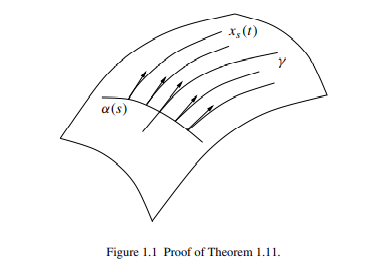
For comparison, and before going further into the Riemannian setting, we briefly present the corresponding Hessian analysis of the distance function from a point in a Lorentzian manifold and its restriction to a spacelike hypersurface. The results can be found in [AHP], where the corresponding Hessian analysis was also carried out, i.e., the analysis of the Lorentzian distance from an achronal spacelike hypersurface in the style of Proposition 3.9. Recall that in Section 3 we also considered

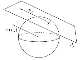
the analysis of the distance from a totally geodesic hypersurface $P$ in the ambient Riemannian manifold $N$.

Let $\left(N^{n+1}, g\right)$ denote an $(n+1)$-dimensional spacetime, that is, a timeoriented Lorentzian manifold of dimension $n+1 \geq 2$. The metric tensor $g$ has index 1 in this case, and, as we did in the Riemannian context, we shall denote it alternatively as $g=\langle,$,$rangle (see, e.g., [O’N] as a standard reference for this section).$
Given $p, q$ two points in $N$, one says that $q$ is in the chronological future of $p$, written $p \ll q$, if there exists a future-directed timelike curve from $p$ to $q$. Similarly, $q$ is in the causal future of $p$, written $p<q$, if there exists a future-directed causal (i.e., nonspacelike) curve from $p$ to $q$.
Then the chronological future $I^{+}(p)$ of a point $p \in N$ is defined as
$$
I^{+}(p)={q \in N: p \ll q} .
$$
The Lorentzian distance function $d: N \times N \rightarrow[0,+\infty]$ for an arbitrary spacetime may fail to be continuous in general, and may also fail to be finite-valued. But there are geometric restrictions that guarantee a good behavior of $d$. For example, globally hyperbolic spacetimes turn out to be the natural class of spacetimes for which the Lorentzian distance function is finite-valued and continuous.

Given a point $p \in N$, one can define the Lorentzian distance function $d_{p}$ :
$M \rightarrow[0,+\infty]$ with respect to $p$ by
$$
d_{p}(q)=d(p, q) .
$$
In order to guarantee the smoothness of $d_{p}$, we need to restrict this function on certain special subsets of $N$. Let $\left.T_{-1} N\right|{p}$ be the following set $$ \left.T{-1} N\right|{p}=\left{v \in T{p} N: v \text { is a future-directed timelike unit vector }\right} .
$$
Define the function $s_{p}:\left.T_{-1} N\right|{p} \rightarrow[0,+\infty]$ by $$ s{p}(v)=\sup \left{t \geq 0: d_{p}\left(\gamma_{v}(t)\right)=t\right},
$$
where $\gamma_{v}:[0, a) \rightarrow N$ is the future inextendible geodesic starting at $p$ with initial velocity $v$. Then we define
$$
\tilde{\mathcal{I}}^{+}(p)=\left{t v: \text { for all }\left.v \in T_{-1} N\right|{p} \text { and } 0{p}(v)\right}
$$
and consider the subset $\mathcal{I}^{+}(p) \subset N$ given by
$$
\mathcal{I}^{+}(p)=\exp {p}\left(\operatorname{int}\left(\tilde{\mathcal{I}}^{+}(p)\right)\right) \subset I^{+}(p) . $$ Observe that the exponential map $$ \exp {p}: \operatorname{int}\left(\tilde{\mathcal{I}}^{+}(p)\right) \rightarrow \mathcal{I}^{+}(p)
$$
is a diffeomorphism and $\mathcal{I}^{+}(p)$ is an open subset (possible empty).
Remark 4.1. When $b \geq 0$, the Lorentzian space form of constant sectional curvature $b$, which we denote as $N_{b}^{n+1}$, is globally hyperbolic and geodesically complete, and every future directed timelike unit geodesic $\gamma_{b}$ in $N_{b}^{n+1}$ realizes the Lorentzian distance between its points. In particular, if $b \geq 0$ then $\mathcal{I}^{+}(p)=I^{+}(p)$ for every point $p \in N_{b}^{n+1}$ (see [EGK, Remark 3.2]).

数学代写|黎曼几何代写Riemannian geometry代考|Concerning the Riemannian Setting and Notation

Returning now to the Riemannian case: Although we indeed do have the possibility of considering 4 basically different settings determined by the choice of $p$ or $V$ as the ‘base’ of our normal domain and the choice of $K_{N} \leq b$ or $K_{N} \geq b$ as the curvature assumption for the ambient space $N$, we will, however, mainly consider the ‘first’ of these. Specifically we will (unless otherwise explicitly stated) apply the following assumptions and denotations:
Definition 5.1. A standard situation encompasses the following:
(1) $P^{m}$ denotes an $m$-dimensional complete minimally immersed submanifold of the Riemannian manifold $N^{n}$. We always assume that $P$ has dimension $m \geq 2 .$
(2) The sectional curvatures of $N$ are assumed to satisfy $K_{N} \leq b, b \in \mathbb{R}$, cf. Proposition $3.10$, equation (3.13).
(3) The intersection of $P$ with a regular ball $B_{R}(p)$ centered at $p \in P$ (cf. Definition 3.4) is denoted by
$$
D_{R}=D_{R}(p)=P^{m} \cap B_{R}(p)
$$
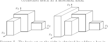
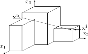
and this is called a minimal extrinsic $R$-ball of $P$ in $N$, see the Figures 3-7 of extrinsic balls, which are cut out from some of the well-known minimal surfaces in $\mathbb{R}^{3}$.
(4) The totally geodesic $m$-dimensional regular $R$-ball centered at $\tilde{p}$ in $\mathbb{K}^{n}(b)$ is denoted by
$$
B_{R}^{b, m}=B_{R}^{b, m}(\tilde{p})
$$
whose boundary is the $(m-1)$-dimensional sphere
$$
\partial B_{R}^{b, m}=S_{R}^{b, m-1}
$$
(5) For any given smooth function $F$ of one real variable we denote
$$
W_{F}(r)=F^{\prime \prime}(r)-F^{\prime}(r) h_{b}(r) \text { for } 0 \leq r \leq R
$$
We may now collect the basic inequalities from our previous analysis as follows.

数学代写|黎曼几何代写Riemannian geometry代考|Green’s Formulae and the Co-area Formula

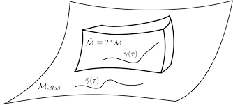
Now we recall the coarea formula. We follow the lines of [Sa] Chapter II, Section 5. Let $(M, g)$ denote a Riemannian manifold and $\Omega$ a precompact domain in $M$. Let $\psi: \Omega \rightarrow \mathbb{R}$ be a smooth function such that $\psi(\Omega)=[a, b]$ with $a<b$. Denote by $\Omega_{0}$ the set of critical points of $\psi$. By Sard’s theorem, the set of critical values $S_{\psi}=\psi\left(\Omega_{0}\right)$ has null measure, and the set of regular values $R_{\psi}=[a, b]-S_{\psi}$ is open. In particular, for any $t \in R_{\psi}=[a, b]-S_{\psi}$, the set $\Gamma(t):=\psi^{-1}(t)$ is a smooth embedded hypersurface in $\Omega$ with $\partial \Gamma(t)=\emptyset$. Since $\Gamma(t) \subseteq \Omega-\Omega_{0}$ then $\nabla \psi$ does not vanish along $\Gamma(t)$; indeed, a unit normal along $\Gamma(t)$ is given by $\nabla \psi /|\nabla \psi|$.
Now we let
$$
\begin{aligned}
&A(t)=\operatorname{Vol}(\Gamma(t)) \
&\Omega(t)={x \in \bar{\Omega} \mid \psi(x)<t} \
&V(t)=\operatorname{Vol}(\Omega(t))
\end{aligned}
$$
Theorem 6.1.
i) For every integrable function $u$ on $\bar{\Omega}$ :
$$
\int_{\Omega} u \cdot|\nabla \psi| d V=\int_{a}^{b}\left(\int_{\Gamma(t)} u d A_{t}\right) d t,
$$
where $d A_{t}$ is the Riemannian volume element defined from the induced metric $g_{t}$ on $\Gamma(t)$ from $g$.
ii) The function $V(t)$ is a smooth function on the regular values of $\psi$ given by:
$$
V(t)=\operatorname{Vol}\left(\Omega_{0} \cap \Omega(t)\right)+\int_{a}^{t}\left(\int_{\Gamma(t)}|\nabla \psi|^{-1} d A_{t}\right)
$$
and its derivative is
$$
\frac{d}{d t} V(t)=\int_{\Gamma(t)}|\nabla \psi|^{-1} d A_{t}
$$

黎曼几何代考

数学代写|黎曼几何代写Riemannian geometry代考|Analysis of Lorentzian Distance Functions

为了比较，在进一步研究黎曼设置之前，我们简要介绍了洛伦兹流形中一点的距离函数的相应 Hessian 分析及其对类空间超曲面的限制。结果可以在[AHP] 中找到，其中也进行了相应的Hessian 分析，即以命题3.9 的风格分析洛伦兹距离与非时间类空间超曲面的距离。回想一下，在第 3 节中，我们还考虑了

与完全测地线超曲面的距离分析磷在环境黎曼流形中ñ.

让(ñn+1,G)表示一个(n+1)维时空，即维的时间导向洛伦兹流形n+1≥2. 度量张量G在这种情况下具有索引 1，并且正如我们在黎曼上下文中所做的那样，我们将其表示为G=⟨,,r一个nGl和(s和和,和.G.,[○′ñ]一个s一个s吨一个nd一个rdr和F和r和nC和F○r吨H一世ss和C吨一世○n).
给定p,q两点在ñ，有人说q是在时间顺序的未来p, 写p≪q, 如果存在一条未来导向的类时曲线p至q. 相似地，q是在因果未来p, 写p<q，如果存在一个未来导向的因果（即非空间）曲线p至q.
然后按时间顺序的未来我+(p)一点的p∈ñ定义为

我+(p)=q∈ñ:p≪q.
洛伦兹距离函数d:ñ×ñ→[0,+∞]因为一个任意的时空通常可能不是连续的，也可能不是有限值的。但是有几何限制可以保证良好的行为d. 例如，全局双曲时空被证明是洛伦兹距离函数是有限值且连续的自然类时空。

给定一个点p∈ñ，可以定义洛伦兹距离函数dp :
米→[0,+∞]关于p经过

dp(q)=d(p,q).
为了保证流畅度dp，我们需要将此函数限制在某些特殊子集上ñ. 让吨−1ñ|p是以下集合

\left.T{-1} N\right|{p}=\left{v \in T{p} N: v \text { 是一个面向未来的类时单位向量 }\right} 。\left.T{-1} N\right|{p}=\left{v \in T{p} N: v \text { 是一个面向未来的类时单位向量 }\right} 。
定义函数sp:吨−1ñ|p→[0,+∞]经过

s{p}(v)=\sup \left{t \geq 0: d_{p}\left(\gamma_{v}(t)\right)=t\right},s{p}(v)=\sup \left{t \geq 0: d_{p}\left(\gamma_{v}(t)\right)=t\right},
在哪里C在:[0,一个)→ñ是未来不可扩展的测地线，开始于p以初速度在. 然后我们定义

\tilde{\mathcal{I}}^{+}(p)=\left{t v: \text { for all }\left.v \in T_{-1} N\right|{p} \text { 和} 0{p}(v)\right}\tilde{\mathcal{I}}^{+}(p)=\left{t v: \text { for all }\left.v \in T_{-1} N\right|{p} \text { 和} 0{p}(v)\right}
并考虑子集我+(p)⊂ñ由

我+(p)=经验⁡p(整数⁡(我~+(p)))⊂我+(p).观察指数图

经验⁡p:整数⁡(我~+(p))→我+(p)
是微分同胚和我+(p)是一个开放子集（可能为空）。
备注 4.1。什么时候b≥0, 等截面曲率的洛伦兹空间形式b, 我们记为ñbn+1, 是全局双曲线和测地线完备的，并且每一个未来有向类时单位测地线Cb在ñbn+1实现其点之间的洛伦兹距离。特别是，如果b≥0然后我+(p)=我+(p)对于每一点p∈ñbn+1（参见 [EGK，备注 3.2]）。

数学代写|黎曼几何代写Riemannian geometry代考|Concerning the Riemannian Setting and Notation

现在回到黎曼案例：虽然我们确实有可能考虑 4 个基本不同的设置，这些设置由p或者在作为我们正常域的“基础”和选择ķñ≤b或者ķñ≥b作为环境空间的曲率假设ñ，但是，我们将主要考虑其中的“第一个”。具体而言，我们将（除非另有明确说明）应用以下假设和表示：
定义 5.1。标准情况包括以下内容：
(1)磷米表示一个米黎曼流形的一维完全最小浸没子流形ñn. 我们总是假设磷有维度米≥2.
(2) 截面曲率ñ假设满足ķñ≤b,b∈R，参见。主张3.10，等式（3.13）。
(3) 交集磷用普通球乙R(p)以p∈磷（参见定义 3.4）表示为

DR=DR(p)=磷米∩乙R(p)
这被称为最小外在R- 球磷在ñ，请参见外部球的图 3-7，它们是从R3.
(4) 完全测地线米维规则R- 球为中心p~在ķn(b)表示为

乙Rb,米=乙Rb,米(p~)
其边界是(米−1)维球

∂乙Rb,米=小号Rb,米−1
(5) 对于任何给定的平滑函数F我们表示的一个实变量

在F(r)=F′′(r)−F′(r)Hb(r) 为了 0≤r≤R
我们现在可以从之前的分析中收集如下的基本不等式。

数学代写|黎曼几何代写Riemannian geometry代考|Green’s Formulae and the Co-area Formula

现在我们回忆一下 coarea 公式。我们遵循 [Sa] 第二章第 5 节的思路。让(米,G)表示黎曼流形和Ω预压缩域米. 让ψ:Ω→R是一个光滑的函数，使得ψ(Ω)=[一个,b]和一个<b. 表示为Ω0的一组临界点ψ. 根据 Sard 定理，临界值的集合小号ψ=ψ(Ω0)具有空度量，以及一组常规值Rψ=[一个,b]−小号ψ开了。特别是，对于任何吨∈Rψ=[一个,b]−小号ψ, 集合Γ(吨):=ψ−1(吨)是一个光滑的嵌入超曲面Ω和∂Γ(吨)=∅. 自从Γ(吨)⊆Ω−Ω0然后∇ψ不会消失Γ(吨); 确实，一个单位正常Γ(吨)是（谁）给的∇ψ/|∇ψ|.
现在我们让

一个(吨)=卷⁡(Γ(吨)) Ω(吨)=X∈Ω¯∣ψ(X)<吨 在(吨)=卷⁡(Ω(吨))
定理 6.1。
i) 对于每个可积函数在上Ω¯ :

∫Ω在⋅|∇ψ|d在=∫一个b(∫Γ(吨)在d一个吨)d吨,
在哪里d一个吨是从诱导度量定义的黎曼体积元素G吨上Γ(吨)从G.
ii) 功能在(吨)是一个关于正则值的平滑函数ψ给出：

在(吨)=卷⁡(Ω0∩Ω(吨))+∫一个吨(∫Γ(吨)|∇ψ|−1d一个吨)
它的导数是

dd吨在(吨)=∫Γ(吨)|∇ψ|−1d一个吨

统计代写请认准statistics-lab™. statistics-lab™为您的留学生涯保驾护航。

金融工程代写

金融工程是使用数学技术来解决金融问题。金融工程使用计算机科学、统计学、经济学和应用数学领域的工具和知识来解决当前的金融问题，以及设计新的和创新的金融产品。

非参数统计代写

非参数统计指的是一种统计方法，其中不假设数据来自于由少数参数决定的规定模型；这种模型的例子包括正态分布模型和线性回归模型。

广义线性模型代考

广义线性模型（GLM）归属统计学领域，是一种应用灵活的线性回归模型。该模型允许因变量的偏差分布有除了正态分布之外的其它分布。

术语 广义线性模型（GLM）通常是指给定连续和/或分类预测因素的连续响应变量的常规线性回归模型。它包括多元线性回归，以及方差分析和方差分析（仅含固定效应）。

有限元方法代写

有限元方法（FEM）是一种流行的方法，用于数值解决工程和数学建模中出现的微分方程。典型的问题领域包括结构分析、传热、流体流动、质量运输和电磁势等传统领域。

有限元是一种通用的数值方法，用于解决两个或三个空间变量的偏微分方程（即一些边界值问题）。为了解决一个问题，有限元将一个大系统细分为更小、更简单的部分，称为有限元。这是通过在空间维度上的特定空间离散化来实现的，它是通过构建对象的网格来实现的：用于求解的数值域，它有有限数量的点。边界值问题的有限元方法表述最终导致一个代数方程组。该方法在域上对未知函数进行逼近。[1] 然后将模拟这些有限元的简单方程组合成一个更大的方程系统，以模拟整个问题。然后，有限元通过变化微积分使相关的误差函数最小化来逼近一个解决方案。

tatistics-lab作为专业的留学生服务机构，多年来已为美国、英国、加拿大、澳洲等留学热门地的学生提供专业的学术服务，包括但不限于Essay代写，Assignment代写，Dissertation代写，Report代写，小组作业代写，Proposal代写，Paper代写，Presentation代写，计算机作业代写，论文修改和润色，网课代做，exam代考等等。写作范围涵盖高中，本科，研究生等海外留学全阶段，辐射金融，经济学，会计学，审计学，管理学等全球99%专业科目。写作团队既有专业英语母语作者，也有海外名校硕博留学生，每位写作老师都拥有过硬的语言能力，专业的学科背景和学术写作经验。我们承诺100%原创，100%专业，100%准时，100%满意。

随机分析代写

随机微积分是数学的一个分支，对随机过程进行操作。它允许为随机过程的积分定义一个关于随机过程的一致的积分理论。这个领域是由日本数学家伊藤清在第二次世界大战期间创建并开始的。

时间序列分析代写

随机过程，是依赖于参数的一组随机变量的全体，参数通常是时间。 随机变量是随机现象的数量表现，其时间序列是一组按照时间发生先后顺序进行排列的数据点序列。通常一组时间序列的时间间隔为一恒定值（如1秒，5分钟，12小时，7天，1年），因此时间序列可以作为离散时间数据进行分析处理。研究时间序列数据的意义在于现实中，往往需要研究某个事物其随时间发展变化的规律。这就需要通过研究该事物过去发展的历史记录，以得到其自身发展的规律。

回归分析代写

多元回归分析渐进（Multiple Regression Analysis Asymptotics）属于计量经济学领域，主要是一种数学上的统计分析方法，可以分析复杂情况下各影响因素的数学关系，在自然科学、社会和经济学等多个领域内应用广泛。

MATLAB代写

MATLAB 是一种用于技术计算的高性能语言。它将计算、可视化和编程集成在一个易于使用的环境中，其中问题和解决方案以熟悉的数学符号表示。典型用途包括：数学和计算算法开发建模、仿真和原型制作数据分析、探索和可视化科学和工程图形应用程序开发，包括图形用户界面构建MATLAB 是一个交互式系统，其基本数据元素是一个不需要维度的数组。这使您可以解决许多技术计算问题，尤其是那些具有矩阵和向量公式的问题，而只需用 C 或 Fortran 等标量非交互式语言编写程序所需的时间的一小部分。MATLAB 名称代表矩阵实验室。MATLAB 最初的编写目的是提供对由 LINPACK 和 EISPACK 项目开发的矩阵软件的轻松访问，这两个项目共同代表了矩阵计算软件的最新技术。MATLAB 经过多年的发展，得到了许多用户的投入。在大学环境中，它是数学、工程和科学入门和高级课程的标准教学工具。在工业领域，MATLAB 是高效研究、开发和分析的首选工具。MATLAB 具有一系列称为工具箱的特定于应用程序的解决方案。对于大多数 MATLAB 用户来说非常重要，工具箱允许您学习和应用专业技术。工具箱是 MATLAB 函数（M 文件）的综合集合，可扩展 MATLAB 环境以解决特定类别的问题。可用工具箱的领域包括信号处理、控制系统、神经网络、模糊逻辑、小波、仿真等。

R语言代写	问卷设计与分析代写
PYTHON代写	回归分析与线性模型代写
MATLAB代写	方差分析与试验设计代写
STATA代写	机器学习/统计学习代写
SPSS代写	计量经济学代写
EVIEWS代写	时间序列分析代写
EXCEL代写	深度学习代写
SQL代写	各种数据建模与可视化代写

如果你也在 怎样代写黎曼几何Riemannian geometry这个学科遇到相关的难题，请随时右上角联系我们的24/7代写客服。

黎曼几何是研究黎曼流形的微分几何学分支，黎曼流形是具有黎曼公制的光滑流形，即在每一点的切线空间上有一个内积，从一点到另一点平滑变化。

statistics-lab™ 为您的留学生涯保驾护航 在代写黎曼几何Riemannian geometry方面已经树立了自己的口碑, 保证靠谱, 高质且原创的统计Statistics代写服务。我们的专家在代写黎曼几何Riemannian geometry代写方面经验极为丰富，各种代写黎曼几何Riemannian geometry相关的作业也就用不着说。

我们提供的黎曼几何Riemannian geometry及其相关学科的代写，服务范围广, 其中包括但不限于:

• Statistical Inference 统计推断
• Statistical Computing 统计计算
• Advanced Probability Theory 高等概率论
• Advanced Mathematical Statistics 高等数理统计学
• (Generalized) Linear Models 广义线性模型
• Statistical Machine Learning 统计机器学习
• Longitudinal Data Analysis 纵向数据分析
• Foundations of Data Science 数据科学基础

数学代写|黎曼几何代写Riemannian geometry代考|Appetizer and Introduction

It is a natural and indeed a classical question to ask: “What is the effective resistance of, say, a hyperboloid or a helicoid if the surface is made of a homogeneous conducting material?”.

In these notes we will study the precise meaning of this and several other related questions and analyze how the answers depend on the curvature and topology of the given surfaces and manifolds. We will focus mainly on minimal submanifolds in ambient spaces which are assumed to have a well-defined upper (or lower) bound on their sectional curvatures.

One key ingredient is the comparison theory for distance functions in such spaces. In particular we establish and use a comparison result for the Laplacian of geometrically restricted distance functions. It is in this setting that we obtain information about such diverse phenomena as diffusion processes, isoperimetric inequalities, Dirichlet eigenvalues, transience, recurrence, and effective resistance of the spaces in question. In this second edition of the present notes we extend those previous findings in four ways: Firstly, we include comparison results for the exit time moment spectrum for compact domains in Riemannian manifolds; Secondly, and most substantially, we report on very recent results obtained by the first and third author together with C. Rosales concerning comparison results for the capacities and the type problem (transient versus recurrent) in weighted Riemannian manifolds; Thirdly we survey how some of the purely Riemannian results on transience and recurrence can be lifted to the setting of spacelike submanifolds in Lorentzian manifolds; Fourthly, the comparison spaces that we employ for some of the new results are typically so-called model spaces, i.e., warped products (gen= eralized surfaces of revolution) where ‘all the geometry’ in each case is determined by a given radial warping function and a given weight function.In a sense, all the different phenomena that we consider are ‘driven’ by the Laplace operator which in turn depends on the background curvatures and the weight function. One key message of this report is that the Laplacian is a particularly ‘swift’ operator – for example on minimal submanifolds in ambient spaces with small sectional curvatures – but depending on the weight functions. Specifically, we observe and report new findings about this behaviour in the contexts of both Riemannian, Lorentzian, and weighted geometries, see Sections 12 and $20-27$. Similar results generally hold true within the intrinsic geometry of the manifolds themselves – often even with Ricci curvature lower bounds (see, e.g., the survey [Zhu]) as a substitute for the specific assumption of a lower bound on sectional curvatures.

数学代写|黎曼几何代写Riemannian geometry代考|The Comparison Setting and Preliminaries

We consider a complete immersed submanifold $P^{m}$ in a Riemannian manifold $N^{n}$, and denote by $\mathrm{D}^{P}$ and $\mathrm{D}^{N}$ the Riemannian connections of $P$ and $N$, respectively. We refer to the excellent general monographs on Riemannian geometry – e.g., [Sa], [CheeE], and [Cha2] – for the basic notions, that will be applied in these notes. In particular we shall be concerned with the second-order behavior of certain functions on $P$ which are obtained by restriction from the ambient space $N$ as displayed in Proposition $3.1$ below. The second-order derivatives are defined in terms of the Hessian operators Hess ${ }^{N}$, Hess ${ }^{P}$ and their traces $\Delta^{N}$ and $\Delta^{P}$, respectively (see, e.g., [Sa] p. 31). The difference between these operators quite naturally involves geometric second-order information about how $P^{m}$ actually sits inside $N^{n}$. This information is provided by the second fundamental form $\alpha$ (resp. the mean curvature $H$ ) of $P$ in $N$ (see [Sa] p. 47). If the functions under consideration are essentially distance functions in $N$ – or suitably modified distance functions then their second-order behavior is strongly influenced by the curvatures of $N$, as is directly expressed by the second variation formula for geodesics ([Sa] p. 90).

As is well known, the ensuing and by now classical comparison theorems for Jacobi fields give rise to the celebrated Toponogov theorems for geodesic triangles and to powerful results concerning the global structure of Riemannian spaces ([Sa], Chapters IV-V). In these notes, however, we shall mainly apply the Jacobi field comparison theory only off the cut loci of the ambient space $N$, or more precisely, within the regular balls of $N$ as defined in Definition $3.4$ below. On the other hand, from the point of view of a given (minimal) submanifold $P$ in $N$, our results for $P$ are semi-global in the sense that they apply to domains which are not necessarily distance-regular within $P$.

数学代写|黎曼几何代写Riemannian geometry代考|Analysis of Riemannian Distance Functions

Let $\mu: N \mapsto \mathbb{R}$ denote a smooth function on $N$. Then the restriction $\tilde{\mu}=\mu_{\left.\right|{P}}$ is a smooth function on $P$ and the respective Hessians $\operatorname{Hess}^{N}(\mu)$ and $\operatorname{Hess}^{P}(\tilde{\mu})$ are related as follows: Proposition $3.1([\mathrm{JK}]$ p. 713$)$. $$ \begin{aligned} \operatorname{Hess}^{P}(\tilde{\mu})(X, Y)=& \operatorname{Hess}^{N}(\mu)(X, Y) \ &+\left\langle\nabla^{N}(\mu), \alpha(X, Y)\right\rangle \end{aligned} $$ for all tangent vectors $X, Y \in T P \subseteq T N$, where $\alpha$ is the second fundamental form of $P$ in $N$. Proof. $$ \begin{aligned} \operatorname{Hess}^{P}(\tilde{\mu})(X, Y) &=\left\langle\mathrm{D}{X}^{P} \nabla^{P} \tilde{\mu}, Y\right\rangle \
&=\left\langle\mathrm{D}{X}^{N} \nabla^{P} \tilde{\mu}-\alpha\left(X, \nabla^{P} \tilde{\mu}\right), Y\right\rangle \ &=\left\langle\mathrm{D}{X}^{N} \nabla^{P} \tilde{\mu}, Y\right\rangle \
&=X\left(\left\langle\nabla^{P} \tilde{\mu}, Y\right\rangle\right)-\left\langle\nabla^{P} \tilde{\mu}, \mathrm{D}{X}^{N} Y\right\rangle \ &=\left\langle\mathrm{D}{X}^{N} \nabla^{N} \mu, Y\right\rangle+\left\langle\left(\nabla^{N} \mu\right)^{\perp}, \mathrm{D}_{X}^{N} Y\right\rangle \
&=\operatorname{Hess}^{N}(\mu)(X, Y)+\left\langle\left(\nabla^{N} \mu\right)^{\perp}, \alpha(X, Y)\right\rangle \
&=\operatorname{Hess}^{N}(\mu)(X, Y)+\left\langle\nabla^{N} \mu, \alpha(X, Y)\right\rangle
\end{aligned}
$$
If we modify $\mu$ to $F \circ \mu$ by a smooth function $F: \mathbb{R} \mapsto \mathbb{R}$, then we get
Lemma 3.2.
$$
\begin{aligned}
\operatorname{Hess}^{N}(F \circ \mu)(X, X)=& F^{\prime \prime}(\mu) \cdot\left\langle\nabla^{N}(\mu), X\right\rangle^{2} \
&+F^{\prime}(\mu) \cdot \operatorname{Hess}^{N}(\mu)(X, X)
\end{aligned}
$$
for all $X \in T N^{n}$

In the following we write $\mu=\tilde{\mu}$. Combining (3.1) and (3.3) then gives
Corollary 3.3.
$$
\begin{aligned}
\operatorname{Hess}^{P}(F \circ \mu)(X, X)=& F^{\prime \prime}(\mu) \cdot\left\langle\nabla^{N}(\mu), X\right\rangle^{2} \
&+F^{\prime}(\mu) \cdot \operatorname{Hess}^{N}(\mu)(X, X) \
&+\left\langle\nabla^{N}(\mu), \alpha(X, X)\right\rangle
\end{aligned}
$$
for all $X \in T P^{m}$.
In what follows the function $\mu$ will always be a distance function in $N$-either from a point $p$ in which case we set $\mu(x)=\operatorname{dist}{N}(p, x)=r(x)$, or from a totally geodesic hypersurface $V^{n-1}$ in $N$ in which case we let $\mu(x)=$ dist ${N}(V, x)=$ $\eta(x)$. The function $F$ will always be chosen, so that $F \circ \mu$ is smooth inside the respective regular balls around $p$ and inside the regular tubes around $V$, which we now define. The sectional curvatures of the two-planes $\Omega$ in the tangent bundle of the ambient space $N$ are denoted by $K_{N}(\Omega)$, see, e.g., [Sa], Section II.3. Concerning the notation: In the following both Hess $^{N}$ and Hess will be used invariantly for both the Hessian in the ambient manifold $N$, as well as in a purely intrinsic context where only $N$ and not any of its submanifolds is under consideration.

黎曼几何代考

数学代写|黎曼几何代写Riemannian geometry代考|Appetizer and Introduction

这是一个自然且确实是经典的问题：“如果表面由均质导电材料制成，例如双曲面或螺旋面的有效电阻是多少？”。

在这些笔记中，我们将研究这个问题和其他几个相关问题的确切含义，并分析答案如何取决于给定曲面和流形的曲率和拓扑结构。我们将主要关注环境空间中的最小子流形，这些子流形假定其截面曲率具有明确定义的上限（或下限）。

一个关键因素是此类空间中距离函数的比较理论。特别是，我们建立并使用了几何限制距离函数的拉普拉斯算子的比较结果。正是在这种情况下，我们获得了有关扩散过程、等周不等式、狄利克雷特征值、瞬变、递归和所讨论空间的有效阻力等多种现象的信息。在本笔记的第二版中，我们以四种方式扩展了这些先前的发现：首先，我们包括黎曼流形中紧域的退出时间矩谱的比较结果；其次，也是最重要的，我们报告了第一作者和第三作者与 C. Rosales 关于加权黎曼流形中容量和类型问题（瞬态与循环）的比较结果；第三，我们调查了一些关于瞬态和递归的纯黎曼结果如何可以提升到洛伦兹流形中的类空间子流形的设置；第四，我们为一些新结果使用的比较空间通常是所谓的模型空间，即翘曲产品（一般化的旋转表面），其中“所有几何形状”在每种情况下都由给定的径向翘曲确定函数和给定的权重函数。在某种意义上，我们考虑的所有不同现象都是由拉普拉斯算子“驱动”的，而拉普拉斯算子又取决于背景曲率和权重函数。本报告的一个关键信息是，拉普拉斯算子是一种特别“快速”的算子——例如在具有小截面曲率的环境空间中的最小子流形上——但取决于权重函数。具体来说，我们在黎曼、洛伦兹和加权几何的背景下观察并报告了关于这种行为的新发现，见第 12 节和20−27. 类似的结果通常在流形本身的内在几何中成立——通常甚至使用 Ricci 曲率下界（参见，例如，调查 [Zhu]）来替代截面曲率下界的特定假设。

数学代写|黎曼几何代写Riemannian geometry代考|The Comparison Setting and Preliminaries

我们考虑一个完全浸入式子流形磷米在黎曼流形中ñn，并表示为D磷和Dñ的黎曼联系磷和ñ， 分别。对于将在这些笔记中应用的基本概念，我们参考了关于黎曼几何的优秀一般专着——例如，[Sa]、[CheeE] 和 [Cha2]。特别是我们将关注某些函数的二阶行为磷通过环境空间的限制获得ñ如提案中所示3.1以下。二阶导数根据 Hessian 算子 Hess 定义ñ, 赫斯磷和他们的踪迹Δñ和Δ磷，分别（参见，例如，[Sa] p. 31）。这些运算符之间的差异很自然地涉及有关如何磷米实际上坐在里面ñn. 此信息由第二个基本形式提供一个（分别是平均曲率H） 的磷在ñ（参见 [Sa] 第 47 页）。如果所考虑的函数本质上是距离函数ñ– 或适当修改的距离函数，则它们的二阶行为受到曲率的强烈影响ñ，正如测地线的第二个变化公式直接表示的那样 ([Sa] p. 90)。

众所周知，Jacobi 场的经典比较定理产生了著名的测地线三角形 Toponogov 定理和关于黎曼空间的全局结构的强大结果（[Sa]，第 IV-V 章）。然而，在这些笔记中，我们将主要应用雅可比场比较理论，仅适用于环境空间的切割轨迹ñ，或者更准确地说，在ñ如定义中所定义3.4以下。另一方面，从给定（最小）子流形的角度来看磷在ñ, 我们的结果为磷是半全局的，因为它们适用于不一定是距离规则的域磷.

数学代写|黎曼几何代写Riemannian geometry代考|Analysis of Riemannian Distance Functions

让μ:ñ↦R表示一个平滑函数ñ. 然后是限制μ~=μ|磷是一个平滑函数磷和各自的黑森州赫斯ñ⁡(μ)和赫斯磷⁡(μ~)相关如下： 命题3.1([Ĵķ]页。713).

赫斯磷⁡(μ~)(X,是)=赫斯ñ⁡(μ)(X,是) +⟨∇ñ(μ),一个(X,是)⟩对于所有切向量X,是∈吨磷⊆吨ñ， 在哪里一个是第二种基本形式磷在ñ. 证明。

赫斯磷⁡(μ~)(X,是)=⟨DX磷∇磷μ~,是⟩ =⟨DXñ∇磷μ~−一个(X,∇磷μ~),是⟩ =⟨DXñ∇磷μ~,是⟩ =X(⟨∇磷μ~,是⟩)−⟨∇磷μ~,DXñ是⟩ =⟨DXñ∇ñμ,是⟩+⟨(∇ñμ)⊥,DXñ是⟩ =赫斯ñ⁡(μ)(X,是)+⟨(∇ñμ)⊥,一个(X,是)⟩ =赫斯ñ⁡(μ)(X,是)+⟨∇ñμ,一个(X,是)⟩
如果我们修改μ至F∘μ通过平滑函数F:R↦R，然后我们得到
引理 3.2。

赫斯ñ⁡(F∘μ)(X,X)=F′′(μ)⋅⟨∇ñ(μ),X⟩2 +F′(μ)⋅赫斯ñ⁡(μ)(X,X)
对所有人X∈吨ñn

下面我们写μ=μ~. 结合 (3.1) 和 (3.3) 得出
推论 3.3。

赫斯磷⁡(F∘μ)(X,X)=F′′(μ)⋅⟨∇ñ(μ),X⟩2 +F′(μ)⋅赫斯ñ⁡(μ)(X,X) +⟨∇ñ(μ),一个(X,X)⟩
对所有人X∈吨磷米.
在下面的函数μ永远是一个距离函数ñ——无论从哪一点p在这种情况下，我们设置μ(X)=距离⁡ñ(p,X)=r(X)，或从完全测地线超曲面在n−1在ñ在这种情况下，我们让μ(X)=距离ñ(在,X)= 这(X). 功能F将始终被选中，因此F∘μ在周围的各个常规球内是光滑的p在周围的常规管内在，我们现在定义。两平面的截面曲率Ω在环境空间的切丛中ñ表示为ķñ(Ω)，参见，例如，[Sa]，第 II.3 节。关于符号：在以下两个赫斯ñ并且 Hess 将不变地用于环境流形中的 Hessianñ，以及在纯粹的内在上下文中，只有ñ并且没有考虑其任何子流形。

统计代写请认准statistics-lab™. statistics-lab™为您的留学生涯保驾护航。

金融工程代写

金融工程是使用数学技术来解决金融问题。金融工程使用计算机科学、统计学、经济学和应用数学领域的工具和知识来解决当前的金融问题，以及设计新的和创新的金融产品。

非参数统计代写

非参数统计指的是一种统计方法，其中不假设数据来自于由少数参数决定的规定模型；这种模型的例子包括正态分布模型和线性回归模型。

广义线性模型代考

广义线性模型（GLM）归属统计学领域，是一种应用灵活的线性回归模型。该模型允许因变量的偏差分布有除了正态分布之外的其它分布。

术语 广义线性模型（GLM）通常是指给定连续和/或分类预测因素的连续响应变量的常规线性回归模型。它包括多元线性回归，以及方差分析和方差分析（仅含固定效应）。

有限元方法代写

有限元方法（FEM）是一种流行的方法，用于数值解决工程和数学建模中出现的微分方程。典型的问题领域包括结构分析、传热、流体流动、质量运输和电磁势等传统领域。

有限元是一种通用的数值方法，用于解决两个或三个空间变量的偏微分方程（即一些边界值问题）。为了解决一个问题，有限元将一个大系统细分为更小、更简单的部分，称为有限元。这是通过在空间维度上的特定空间离散化来实现的，它是通过构建对象的网格来实现的：用于求解的数值域，它有有限数量的点。边界值问题的有限元方法表述最终导致一个代数方程组。该方法在域上对未知函数进行逼近。[1] 然后将模拟这些有限元的简单方程组合成一个更大的方程系统，以模拟整个问题。然后，有限元通过变化微积分使相关的误差函数最小化来逼近一个解决方案。

tatistics-lab作为专业的留学生服务机构，多年来已为美国、英国、加拿大、澳洲等留学热门地的学生提供专业的学术服务，包括但不限于Essay代写，Assignment代写，Dissertation代写，Report代写，小组作业代写，Proposal代写，Paper代写，Presentation代写，计算机作业代写，论文修改和润色，网课代做，exam代考等等。写作范围涵盖高中，本科，研究生等海外留学全阶段，辐射金融，经济学，会计学，审计学，管理学等全球99%专业科目。写作团队既有专业英语母语作者，也有海外名校硕博留学生，每位写作老师都拥有过硬的语言能力，专业的学科背景和学术写作经验。我们承诺100%原创，100%专业，100%准时，100%满意。

随机分析代写

随机微积分是数学的一个分支，对随机过程进行操作。它允许为随机过程的积分定义一个关于随机过程的一致的积分理论。这个领域是由日本数学家伊藤清在第二次世界大战期间创建并开始的。

时间序列分析代写

随机过程，是依赖于参数的一组随机变量的全体，参数通常是时间。 随机变量是随机现象的数量表现，其时间序列是一组按照时间发生先后顺序进行排列的数据点序列。通常一组时间序列的时间间隔为一恒定值（如1秒，5分钟，12小时，7天，1年），因此时间序列可以作为离散时间数据进行分析处理。研究时间序列数据的意义在于现实中，往往需要研究某个事物其随时间发展变化的规律。这就需要通过研究该事物过去发展的历史记录，以得到其自身发展的规律。

回归分析代写

多元回归分析渐进（Multiple Regression Analysis Asymptotics）属于计量经济学领域，主要是一种数学上的统计分析方法，可以分析复杂情况下各影响因素的数学关系，在自然科学、社会和经济学等多个领域内应用广泛。

MATLAB代写

MATLAB 是一种用于技术计算的高性能语言。它将计算、可视化和编程集成在一个易于使用的环境中，其中问题和解决方案以熟悉的数学符号表示。典型用途包括：数学和计算算法开发建模、仿真和原型制作数据分析、探索和可视化科学和工程图形应用程序开发，包括图形用户界面构建MATLAB 是一个交互式系统，其基本数据元素是一个不需要维度的数组。这使您可以解决许多技术计算问题，尤其是那些具有矩阵和向量公式的问题，而只需用 C 或 Fortran 等标量非交互式语言编写程序所需的时间的一小部分。MATLAB 名称代表矩阵实验室。MATLAB 最初的编写目的是提供对由 LINPACK 和 EISPACK 项目开发的矩阵软件的轻松访问，这两个项目共同代表了矩阵计算软件的最新技术。MATLAB 经过多年的发展，得到了许多用户的投入。在大学环境中，它是数学、工程和科学入门和高级课程的标准教学工具。在工业领域，MATLAB 是高效研究、开发和分析的首选工具。MATLAB 具有一系列称为工具箱的特定于应用程序的解决方案。对于大多数 MATLAB 用户来说非常重要，工具箱允许您学习和应用专业技术。工具箱是 MATLAB 函数（M 文件）的综合集合，可扩展 MATLAB 环境以解决特定类别的问题。可用工具箱的领域包括信号处理、控制系统、神经网络、模糊逻辑、小波、仿真等。

R语言代写	问卷设计与分析代写
PYTHON代写	回归分析与线性模型代写
MATLAB代写	方差分析与试验设计代写
STATA代写	机器学习/统计学习代写
SPSS代写	计量经济学代写
EVIEWS代写	时间序列分析代写
EXCEL代写	深度学习代写
SQL代写	各种数据建模与可视化代写

如果你也在 怎样代写黎曼几何Riemannian geometry这个学科遇到相关的难题，请随时右上角联系我们的24/7代写客服。

黎曼几何是研究黎曼流形的微分几何学分支，黎曼流形是具有黎曼公制的光滑流形，即在每一点的切线空间上有一个内积，从一点到另一点平滑变化。

statistics-lab™ 为您的留学生涯保驾护航 在代写黎曼几何Riemannian geometry方面已经树立了自己的口碑, 保证靠谱, 高质且原创的统计Statistics代写服务。我们的专家在代写黎曼几何Riemannian geometry代写方面经验极为丰富，各种代写黎曼几何Riemannian geometry相关的作业也就用不着说。

我们提供的黎曼几何Riemannian geometry及其相关学科的代写，服务范围广, 其中包括但不限于:

• Statistical Inference 统计推断
• Statistical Computing 统计计算
• Advanced Probability Theory 高等概率论
• Advanced Mathematical Statistics 高等数理统计学
• (Generalized) Linear Models 广义线性模型
• Statistical Machine Learning 统计机器学习
• Longitudinal Data Analysis 纵向数据分析
• Foundations of Data Science 数据科学基础

数学代写|黎曼几何代写Riemannian geometry代考|The Minimal Control and the Length of an Admissible Curve

We start by defining the sub-Riemannian norm for vectors that belong to the distribution of a sub-Riemannian manifold.

Definition 3.8 Let $v \in \mathcal{D}{q}$. We define the sub-Riemannian norm of $v$ as follows: $$ |v|:=\min \left{|u|, u \in U{q} \text { s.t. } v=f(q, u)\right} .
$$
Notice that since $f$ is linear with respect to $u$, the minimum in $(3.9)$ is always attained at a unique point. Indeed, the condition $f(q, \cdot)=v$ defines an affine subspace of $U_{q}$ (which is nonempty since $v \in \mathcal{D}_{q}$ ) and the minimum in (3.9) is uniquely attained at the orthogonal projection of the origin onto this subspace (see Figure 3.2).

Exercise 3.9 Show that $|\cdot|$ is a norm in $\mathcal{D}{q}$. Moreover prove that it satisfies the parallelogram law, i.e., it is induced by a scalar product $\langle\cdot \mid \cdot\rangle{q}$ on $\mathcal{D}{q}$ that can be recovered by the polarization identity $$ \langle v \mid w\rangle{q}=\frac{1}{4}|v+w|^{2}-\frac{1}{4}|v-w|^{2}, \quad v, w \in \mathcal{D}{q} . $$ Exercise $3.10$ Let $u{1}, \ldots, u_{m} \in U_{q}$ be an orthonormal basis for $U_{q}$. Define $v_{i}=f\left(q, u_{i}\right)$. Show that if $f(q, \cdot)$ is injective then $v_{1}, \ldots, v_{m}$ is an orthonormal basis for $\mathcal{D}_{q}$.

An admissible curve $\gamma:[0, T] \rightarrow M$ is Lipschitz, hence differentiable at almost every point. Hence the unique control $t \mapsto u^{*}(t)$ associated with $\gamma$ and realizing the minimum in $(3.9)$ is well defined a.e. on $[0, T]$.

数学代写|黎曼几何代写Riemannian geometry代考|Equivalence of Sub-Riemannian Structures

In this section we introduce the notion of the equivalence of sub-Riemannian structures on the same base manifold $M$ and the notion of isometry between sub-Riemannian manifolds.

Definition $3.18$ Let $(\mathbf{U}, f),\left(\mathbf{U}^{\prime}, f^{\prime}\right)$ be two sub-Riemannian structures on a smooth manifold $M$. They are said to be equivalent as distributions if the following conditions hold:

(i) there exist a Euclidean bundle $\mathbf{V}$ and two surjective vector bundle morphisms $p: \mathbf{V} \rightarrow \mathbf{U}$ and $p^{\prime}: \mathbf{V} \rightarrow \mathbf{U}^{\prime}$ such that the following diagram is commutative:

The structures $(\mathbf{U}, f)$ and $\left(\mathbf{U}^{\prime}, f^{\prime}\right)$ are said to be equivalent as sub-Riemannian structures (or simply equivalent) if (i) is satisfied and moreover
(ii) the projections $p, p^{\prime}$ are compatible with the scalar product, i.e., it holds that
$$
\begin{aligned}
|u| &=\min {|v|, p(v)=u}, & \forall u \in \mathbf{U}, \
\left|u^{\prime}\right| &=\min \left{|v|, p^{\prime}(v)=u^{\prime}\right}, & \forall u^{\prime} \in \mathbf{U}^{\prime} .
\end{aligned}
$$
Remark $3.19$ If $(\mathbf{U}, f)$ and $\left(\mathbf{U}^{\prime}, f^{\prime}\right)$ arc cquivalcnt as sub-Ricmannian structures on $M$ then:
(a) the distributions $\mathcal{D}{q}$ and $\mathcal{D}{q}^{\prime}$ defined by $f$ and $f^{\prime}$ coincide, since $f\left(U_{q}\right)=f^{\prime}\left(U_{q}^{\prime}\right)$ for all $q \in M$;
(b) for each $w \in \mathcal{D}_{q}$ we have $|w|=|w|^{\prime}$, where $|\cdot|$ and $|\cdot|^{\prime}$ are the norms induced by $(\mathbf{U}, f)$ and $\left(\mathbf{U}^{\prime}, f^{\prime}\right)$ respectively.
In particular the lengths of admissible curves for two equivalent subRiemannian structures are the same.

Exercise 3.20 Prove that $(M, \mathbf{U}, f)$ and $\left(M, \mathbf{U}^{\prime}, f^{\prime}\right)$ are equivalent as distributions if and only if the moduli of the horizontal vector fields $\mathcal{D}$ and $\mathcal{D}^{\prime}$ coincide.

数学代写|黎曼几何代写Riemannian geometry代考|Sub-Riemannian Distance

In this section we introduce the sub-Riemannian distance and prove the Rashevskii-Chow theorem.

Recall that, thanks to the results of Section 3.1.4, in what follows we can assume that the sub-Riemannian structure on $M$ is free, with generating family $\mathcal{F}=\left{f_{1}, \ldots, f_{m}\right}$. Notice that, by the definition of a sub-Riemannian manifold, $M$ is assumed to be connected and $\mathcal{F}$ is assumed to be bracketgenerating.

Definition 3.30 Let $M$ be a sub-Riemannian manifold and $q_{0}, q_{1} \in M$. The sub-Riemannian distance (or Carnot-Carathéodory distance) between $q_{0}$ and $q_{1}$ is
$d\left(q_{0}, q_{1}\right)=\inf \left{\ell(\gamma) \mid \gamma:[0, T] \rightarrow M\right.$ admissible, $\left.\gamma(0)=q_{0}, \gamma(T)=q_{1}\right} .$
We now state the main result of this section.
Theorem $3.31$ (Rashevskii-Chow) Let $M$ be a sub-Riemannian manifold. Then
(i) $(M, d)$ is a metric space,
(ii) the topology induced by $(M, d)$ is equivalent to the manifold topology.
In particular, $d: M \times M \rightarrow \mathbb{R}$ is continuous.
One of the main consequences of this result is that, thanks to the bracketgenerating condition, for every $q_{0}, q_{1} \in M$ there exists an admissible curve that joins them. Hence $d\left(q_{0}, q_{1}\right)<+\infty$.

In what follows $B(q, r)$ (sometimes denoted also $B_{r}(q)$ ) is the (open) subRiemannian ball of radius $r$ and center $q$ :
$$
B(q, r):=\left{q^{\prime} \in M \mid d\left(q, q^{\prime}\right)<r\right} .
$$

黎曼几何代考

数学代写|黎曼几何代写Riemannian geometry代考|The Minimal Control and the Length of an Admissible Curve

我们首先为属于亚黎曼流形分布的向量定义亚黎曼范数。

定义 3.8 让在∈Dq. 我们定义的亚黎曼范数在如下：

|v|:=\min \left{|u|, u \in U{q} \text { st } v=f(q, u)\right} 。|v|:=\min \left{|u|, u \in U{q} \text { st } v=f(q, u)\right} 。
请注意，由于F是线性的在, 中的最小值(3.9)总是在一个独特的点上获得。确实，条件F(q,⋅)=在定义了一个仿射子空间在q（这是非空的，因为在∈Dq) 并且 (3.9) 中的最小值是在原点到该子空间的正交投影处唯一获得的（参见图 3.2）。

练习 3.9 证明|⋅|是一个规范Dq. 进一步证明它满足平行四边形定律，即它是由一个标量积导出的⟨⋅∣⋅⟩q上Dq可以通过极化同一性恢复

⟨在∣在⟩q=14|在+在|2−14|在−在|2,在,在∈Dq.锻炼3.10让在1,…,在米∈在q是一个正交基在q. 定义在一世=F(q,在一世). 证明如果F(q,⋅)是内射的在1,…,在米是一个正交基Dq.

可接受的曲线C:[0,吨]→米是 Lipschitz，因此几乎在每个点都是可微的。因此，独特的控制吨↦在∗(吨)有关联C并实现最小化(3.9)定义明确 ae on[0,吨].

数学代写|黎曼几何代写Riemannian geometry代考|Equivalence of Sub-Riemannian Structures

在本节中，我们介绍了相同基础流形上的亚黎曼结构等价的概念米以及亚黎曼流形之间的等距概念。

定义3.18让(在,F),(在′,F′)是光滑流形上的两个亚黎曼结构米. 如果满足以下条件，则称它们与分布等效：

(i) 存在欧几里得丛在和两个满射向量丛态射p:在→在和p′:在→在′使得下图是可交换的：

结构(在,F)和(在′,F′)如果满足 (i) 并且
(ii)p,p′与标量积兼容，即它认为

\begin{对齐} |u| &=\min {|v|, p(v)=u}, & \forall u \in \mathbf{U}, \ \left|u^{\prime}\right| &=\min \left{|v|, p^{\prime}(v)=u^{\prime}\right}, & \forall u^{\prime} \in \mathbf{U}^{\主要} 。\end{对齐}\begin{对齐} |u| &=\min {|v|, p(v)=u}, & \forall u \in \mathbf{U}, \ \left|u^{\prime}\right| &=\min \left{|v|, p^{\prime}(v)=u^{\prime}\right}, & \forall u^{\prime} \in \mathbf{U}^{\主要} 。\end{对齐}
评论3.19如果(在,F)和(在′,F′)arc cquivalcnt 作为亚 Ricmannian 结构米那么：
(a) 分布Dq和Dq′被定义为F和F′巧合，因为F(在q)=F′(在q′)对所有人q∈米;
(b) 对于每个在∈Dq我们有|在|=|在|′， 在哪里|⋅|和|⋅|′规范是由(在,F)和(在′,F′)分别。
特别是两个等效亚黎曼结构的容许曲线长度是相同的。

练习 3.20 证明(米,在,F)和(米,在′,F′)当且仅当水平向量场的模量与分布等价D和D′重合。

数学代写|黎曼几何代写Riemannian geometry代考|Sub-Riemannian Distance

在本节中，我们将介绍亚黎曼距离并证明 Rashevskii-Chow 定理。

回想一下，由于第 3.1.4 节的结果，在下面我们可以假设米是免费的，有生成家庭\mathcal{F}=\left{f_{1}, \ldots, f_{m}\right}\mathcal{F}=\left{f_{1}, \ldots, f_{m}\right}. 请注意，根据亚黎曼流形的定义，米假定连接和F假定为括号生成。

定义 3.30 让米是一个亚黎曼流形并且q0,q1∈米. 之间的亚黎曼距离（或 Carnot-Carathéodory 距离）q0和q1是
d\left(q_{0}, q_{1}\right)=\inf \left{\ell(\gamma) \mid \gamma:[0, T] \rightarrow M\right.$ 可接受，$\left .\gamma(0)=q_{0}, \gamma(T)=q_{1}\right} 。d\left(q_{0}, q_{1}\right)=\inf \left{\ell(\gamma) \mid \gamma:[0, T] \rightarrow M\right.$ 可接受，$\left .\gamma(0)=q_{0}, \gamma(T)=q_{1}\right} 。
我们现在陈述本节的主要结果。
定理3.31(Rashevskii-Chow) 让米是一个亚黎曼流形。那么
（一）(米,d)是一个度量空间，
（ii）由(米,d)等价于流形拓扑。
尤其是，d:米×米→R是连续的。
这个结果的主要结果之一是，由于括号生成条件，对于每个q0,q1∈米存在一条连接它们的允许曲线。因此d(q0,q1)<+∞.

在接下来的乙(q,r)（有时也表示乙r(q)) 是半径的（开）亚黎曼球r和中心q :

B(q, r):=\left{q^{\prime} \in M \mid d\left(q, q^{\prime}\right)<r\right} 。

统计代写请认准statistics-lab™. statistics-lab™为您的留学生涯保驾护航。

金融工程代写

金融工程是使用数学技术来解决金融问题。金融工程使用计算机科学、统计学、经济学和应用数学领域的工具和知识来解决当前的金融问题，以及设计新的和创新的金融产品。

非参数统计代写

非参数统计指的是一种统计方法，其中不假设数据来自于由少数参数决定的规定模型；这种模型的例子包括正态分布模型和线性回归模型。

广义线性模型代考

广义线性模型（GLM）归属统计学领域，是一种应用灵活的线性回归模型。该模型允许因变量的偏差分布有除了正态分布之外的其它分布。

术语 广义线性模型（GLM）通常是指给定连续和/或分类预测因素的连续响应变量的常规线性回归模型。它包括多元线性回归，以及方差分析和方差分析（仅含固定效应）。

有限元方法代写

有限元方法（FEM）是一种流行的方法，用于数值解决工程和数学建模中出现的微分方程。典型的问题领域包括结构分析、传热、流体流动、质量运输和电磁势等传统领域。

有限元是一种通用的数值方法，用于解决两个或三个空间变量的偏微分方程（即一些边界值问题）。为了解决一个问题，有限元将一个大系统细分为更小、更简单的部分，称为有限元。这是通过在空间维度上的特定空间离散化来实现的，它是通过构建对象的网格来实现的：用于求解的数值域，它有有限数量的点。边界值问题的有限元方法表述最终导致一个代数方程组。该方法在域上对未知函数进行逼近。[1] 然后将模拟这些有限元的简单方程组合成一个更大的方程系统，以模拟整个问题。然后，有限元通过变化微积分使相关的误差函数最小化来逼近一个解决方案。

tatistics-lab作为专业的留学生服务机构，多年来已为美国、英国、加拿大、澳洲等留学热门地的学生提供专业的学术服务，包括但不限于Essay代写，Assignment代写，Dissertation代写，Report代写，小组作业代写，Proposal代写，Paper代写，Presentation代写，计算机作业代写，论文修改和润色，网课代做，exam代考等等。写作范围涵盖高中，本科，研究生等海外留学全阶段，辐射金融，经济学，会计学，审计学，管理学等全球99%专业科目。写作团队既有专业英语母语作者，也有海外名校硕博留学生，每位写作老师都拥有过硬的语言能力，专业的学科背景和学术写作经验。我们承诺100%原创，100%专业，100%准时，100%满意。

随机分析代写

随机微积分是数学的一个分支，对随机过程进行操作。它允许为随机过程的积分定义一个关于随机过程的一致的积分理论。这个领域是由日本数学家伊藤清在第二次世界大战期间创建并开始的。

时间序列分析代写

随机过程，是依赖于参数的一组随机变量的全体，参数通常是时间。 随机变量是随机现象的数量表现，其时间序列是一组按照时间发生先后顺序进行排列的数据点序列。通常一组时间序列的时间间隔为一恒定值（如1秒，5分钟，12小时，7天，1年），因此时间序列可以作为离散时间数据进行分析处理。研究时间序列数据的意义在于现实中，往往需要研究某个事物其随时间发展变化的规律。这就需要通过研究该事物过去发展的历史记录，以得到其自身发展的规律。

回归分析代写

多元回归分析渐进（Multiple Regression Analysis Asymptotics）属于计量经济学领域，主要是一种数学上的统计分析方法，可以分析复杂情况下各影响因素的数学关系，在自然科学、社会和经济学等多个领域内应用广泛。

MATLAB代写

MATLAB 是一种用于技术计算的高性能语言。它将计算、可视化和编程集成在一个易于使用的环境中，其中问题和解决方案以熟悉的数学符号表示。典型用途包括：数学和计算算法开发建模、仿真和原型制作数据分析、探索和可视化科学和工程图形应用程序开发，包括图形用户界面构建MATLAB 是一个交互式系统，其基本数据元素是一个不需要维度的数组。这使您可以解决许多技术计算问题，尤其是那些具有矩阵和向量公式的问题，而只需用 C 或 Fortran 等标量非交互式语言编写程序所需的时间的一小部分。MATLAB 名称代表矩阵实验室。MATLAB 最初的编写目的是提供对由 LINPACK 和 EISPACK 项目开发的矩阵软件的轻松访问，这两个项目共同代表了矩阵计算软件的最新技术。MATLAB 经过多年的发展，得到了许多用户的投入。在大学环境中，它是数学、工程和科学入门和高级课程的标准教学工具。在工业领域，MATLAB 是高效研究、开发和分析的首选工具。MATLAB 具有一系列称为工具箱的特定于应用程序的解决方案。对于大多数 MATLAB 用户来说非常重要，工具箱允许您学习和应用专业技术。工具箱是 MATLAB 函数（M 文件）的综合集合，可扩展 MATLAB 环境以解决特定类别的问题。可用工具箱的领域包括信号处理、控制系统、神经网络、模糊逻辑、小波、仿真等。

R语言代写	问卷设计与分析代写
PYTHON代写	回归分析与线性模型代写
MATLAB代写	方差分析与试验设计代写
STATA代写	机器学习/统计学习代写
SPSS代写	计量经济学代写
EVIEWS代写	时间序列分析代写
EXCEL代写	深度学习代写
SQL代写	各种数据建模与可视化代写

如果你也在 怎样代写黎曼几何Riemannian geometry这个学科遇到相关的难题，请随时右上角联系我们的24/7代写客服。

黎曼几何是研究黎曼流形的微分几何学分支，黎曼流形是具有黎曼公制的光滑流形，即在每一点的切线空间上有一个内积，从一点到另一点平滑变化。

statistics-lab™ 为您的留学生涯保驾护航 在代写黎曼几何Riemannian geometry方面已经树立了自己的口碑, 保证靠谱, 高质且原创的统计Statistics代写服务。我们的专家在代写黎曼几何Riemannian geometry代写方面经验极为丰富，各种代写黎曼几何Riemannian geometry相关的作业也就用不着说。

我们提供的黎曼几何Riemannian geometry及其相关学科的代写，服务范围广, 其中包括但不限于:

• Statistical Inference 统计推断
• Statistical Computing 统计计算
• Advanced Probability Theory 高等概率论
• Advanced Mathematical Statistics 高等数理统计学
• (Generalized) Linear Models 广义线性模型
• Statistical Machine Learning 统计机器学习
• Longitudinal Data Analysis 纵向数据分析
• Foundations of Data Science 数据科学基础

数学代写|黎曼几何代写Riemannian geometry代考|Vector Bundles

Heuristically, a smooth vector bundle on a smooth manifold $M$ is a smooth family of vector spaces parametrized by points in $M$.

Definition 2.47 Let $M$ be an $n$-dimensional manifold. A smooth vector bundle of rank $k$ over $M$ is a smooth manifold $E$ with a surjective smooth map $\pi: E \rightarrow M$ such that:
(i) the set $E_{q}:=\pi^{-1}(q)$, the $f$ iber of $E$ at $q$, is a $k$-dimensional vector space;
(ii) for every $q \in M$ there exist a neighborhood $O_{q}$ of $q$ and a linear-on-fibers diffeomorphism (called a local trivialization) $\psi: \pi^{-1}\left(O_{q}\right) \rightarrow O_{q} \times \mathbb{R}^{k}$ such that the following diagram commutes:
The space $E$ is called total space and $M$ is the base of the vector bundle. We will refer to $\pi$ as the canonical projection, and rank $E$ will denote the rank of the bundle.
Remark $2.48$ A vector bundle $E$, as a smooth manifold, has dimension
$$
\operatorname{dim} E=\operatorname{dim} M+\operatorname{rank} E=n+k .
$$
In the case when there exists a global trivialization map (i.e., when one can choose a local trivialization with $O_{q}=M$ for all $q \in M$ ), then $E$ is diffeomorphic to $M \times \mathbb{R}^{k}$ and we say that $E$ is trivializable.

Example 2.49 For any smooth $n$-dimensional manifold $M$, the tangent bundle $T M$, defined as the disjoint union of the tangent spaces at all points of $M$,
$$
T M=\bigcup_{q \in M} T_{q} M,
$$
has the natural structure of a $2 n$-dimensional smooth manifold, equipped with the vector bundle structure (of rank $n$ ) induced by the canonical projection map
$$
\pi: T M \rightarrow M, \quad \pi(v)=q \quad \text { if } \quad v \in T_{q} M .
$$
In the same way one can consider the cotangent bundle $T^{} M$, defined as $$ T^{} M=\bigcup_{q \in M} T_{q}^{*} M .
$$

数学代写|黎曼几何代写Riemannian geometry代考|Submersions and Level Sets of Smooth Maps

If $\varphi: M \rightarrow N$ is a smooth map, we define the rank of $\varphi$ at $q \in M$ to be the rank of the linear map $\varphi_{*, q}: T_{q} M \rightarrow T_{\varphi(q)} N$. It is, of course, just the rank of the matrix of partial derivatives of $\varphi$ in any coordinate chart, or the dimension

of $\operatorname{im}\left(\varphi_{*, q}\right) \subset T_{\varphi(q)} N$. If $\varphi$ has the same rank $k$ at every point, we say $\varphi$ has constant rank and write rank $\varphi=k$.

An immersion is a smooth map $\varphi: M \rightarrow N$ with the property that $\varphi_{}$ is injective at each point (or equivalently $\operatorname{rank} \varphi=\operatorname{dim} M$ ). Similarly, a submersion is a smooth map $\varphi: M \rightarrow N$ such that $\varphi_{}$ is surjective at each point (equivalently, $\operatorname{rank} \varphi=\operatorname{dim} N$ ).

Theorem $2.56$ (Rank theorem) Suppose that $M$ and $N$ are smooth manifolds of dimensions $m$ and $n$ respectively and that $\varphi: M \rightarrow N$ is a smooth map with constant rank $k$ in a neighborhood of $q \in M$. Then there exist coordinates $\left(x_{1}, \ldots, x_{m}\right)$ centered at $q$ and $\left(y_{1}, \ldots, y_{n}\right)$ centered at $\varphi(q)$ in which $\varphi$ has the following coordinate representation:
$$
\varphi\left(x_{1}, \ldots, x_{m}\right)=\left(x_{1}, \ldots, x_{k}, 0, \ldots, 0\right) .
$$
Remark $2.57$ The previous theorem can be rephrased in the following way.
Let $\varphi: M \rightarrow N$ be a smooth map between two smooth manifolds. Then the following are equivalent:
(i) $\varphi$ has constant rank in a neighborhood of $q \in M$;
(ii) there exist coordinates near $q \in M$ and $\varphi(q) \in N$ in which the coordinate representation of $\varphi$ is linear.

In the case of a submersion, from Theorem $2.56$ one can deduce the following result.

数学代写|黎曼几何代写Riemannian geometry代考|Basic Definitions

We start by introducing a bracket-generating family of vector fields.
Definition $3.1$ Let $M$ be a smouth manifold and let $\mathcal{F} \subset \operatorname{Vec}(M)$ be a family of smooth vector fields. The Lie algebra generated by $\mathcal{F}$ is the smallest subalgebra of $\operatorname{Vec}(M)$ containing $\mathcal{F}$, namely
$$
\operatorname{Lie} \mathcal{F}:=\operatorname{span}\left{\left[X_{1}, \ldots,\left[X_{j-1}, X_{j}\right]\right], X_{i} \in \mathcal{F}, j \in \mathbb{N}\right}
$$
We will say that $\mathcal{F}$ is bracket-generating (or that it satisfies the Hörmander condition) if
$$
\operatorname{Lie}{q} \mathcal{F}:={X(q), X \in \text { Lie } \mathcal{F}}=T{q} M, \quad \forall q \in M
$$

Moreover, for $s \in \mathbb{N}$, we define
$$
\operatorname{Lie}^{s} \mathcal{F}:=\operatorname{span}\left{\left[X_{1}, \ldots,\left[X_{j-1}, X_{j}\right]\right], X_{i} \in \mathcal{F}, j \leq s\right}
$$
We say that the family $\mathcal{F}$ has step s at $q$ if $s \in \mathbb{N}$ is the minimal integer satisfying
$$
\operatorname{Lie}{q}^{s} \mathcal{F}:=\left{X(q) X \in \operatorname{Lie}^{s} \mathcal{F}\right}=T{q} M
$$
Notice that, in general, the step $s$ may depend on the point on $M$ and that $s=s(q)$ can be unbounded on $M$ even for bracket-generating families.

黎曼几何代考

数学代写|黎曼几何代写Riemannian geometry代考|Vector Bundles

启发式地，光滑流形上的光滑向量丛米是由点参数化的向量空间的平滑族米.

定义 2.47 让米豆n维流形。秩的平滑向量丛ķ超过米是一个光滑的流形和具有满射平滑图圆周率:和→米这样：
(i) 集合和q:=圆周率−1(q)， 这F伊伯尔和在q, 是一个ķ维向量空间；
(ii) 对于每个q∈米有一个社区○q的q和纤维上的线性微分同胚（称为局部平凡化）ψ:圆周率−1(○q)→○q×Rķ使得下图通勤：
空间和称为总空间和米是向量丛的基。我们将参考圆周率作为规范投影，并排名和将表示捆绑的等级。
评论2.48向量束和，作为一个光滑流形，有维数

暗淡⁡和=暗淡⁡米+秩⁡和=n+ķ.
在存在全局平凡化映射的情况下（即，当人们可以选择局部平凡化时○q=米对所有人q∈米）， 然后和微分同胚于米×Rķ我们说和是微不足道的。

例 2.49 对于任何平滑n维流形米, 切丛吨米，定义为在所有点的切空间的不相交并集米,

吨米=⋃q∈米吨q米,
具有a的自然结构2n维光滑流形，配备向量丛结构（秩n) 由正则投影图诱导

圆周率:吨米→米,圆周率(在)=q 如果 在∈吨q米.
以同样的方式可以考虑余切丛吨米， 定义为

吨米=⋃q∈米吨q∗米.

数学代写|黎曼几何代写Riemannian geometry代考|Submersions and Level Sets of Smooth Maps

如果披:米→ñ是一个光滑的地图，我们定义披在q∈米成为线性映射的秩披∗,q:吨q米→吨披(q)ñ. 当然，它只是偏导数矩阵的秩披在任何坐标图中，或维度

的在里面⁡(披∗,q)⊂吨披(q)ñ. 如果披排名相同ķ在每一点，我们说披具有恒定等级和写入等级披=ķ.

沉浸式是一张平滑的地图披:米→ñ与财产披在每一点都是单射的（或等价的秩⁡披=暗淡⁡米）。同样，一个submersion是一个平滑的地图披:米→ñ这样披在每一点上都是满射的（等价地，秩⁡披=暗淡⁡ñ ).

定理2.56（秩定理）假设米和ñ是维度的光滑流形米和n分别和那个披:米→ñ是具有恒定秩的平滑映射ķ在附近q∈米. 那么存在坐标(X1,…,X米)以q和(是1,…,是n)以披(q)其中披具有以下坐标表示：

披(X1,…,X米)=(X1,…,Xķ,0,…,0).
评论2.57前面的定理可以改写如下。
让披:米→ñ是两个光滑流形之间的光滑映射。那么以下是等价的：
(i)披在附近有恒定的排名q∈米;
(ii) 附近有坐标q∈米和披(q)∈ñ其中的坐标表示披是线性的。

在浸没的情况下，从定理2.56可以推导出以下结果。

数学代写|黎曼几何代写Riemannian geometry代考|Basic Definitions

我们首先介绍一个生成括号的向量场族。
定义3.1让米做一个流形，让F⊂一个东西⁡(米)是一个光滑向量场族。李代数由F是的最小子代数一个东西⁡(米)包含F，即

\operatorname{Lie} \mathcal{F}:=\operatorname{span}\left{\left[X_{1}, \ldots,\left[X_{j-1}, X_{j}\right]\right ], X_{i} \in \mathcal{F}, j \in \mathbb{N}\right}\operatorname{Lie} \mathcal{F}:=\operatorname{span}\left{\left[X_{1}, \ldots,\left[X_{j-1}, X_{j}\right]\right ], X_{i} \in \mathcal{F}, j \in \mathbb{N}\right}
我们会说F是括号生成的（或者它满足 Hörmander 条件）如果

说谎⁡qF:=X(q),X∈ 说谎 F=吨q米,∀q∈米

此外，对于s∈ñ，我们定义

\operatorname{Lie}^{s} \mathcal{F}:=\operatorname{span}\left{\left[X_{1}, \ldots,\left[X_{j-1}, X_{j}\对]\right], X_{i} \in \mathcal{F}, j \leq s\right}\operatorname{Lie}^{s} \mathcal{F}:=\operatorname{span}\left{\left[X_{1}, \ldots,\left[X_{j-1}, X_{j}\对]\right], X_{i} \in \mathcal{F}, j \leq s\right}
我们说家庭F有步骤 s 在q如果s∈ñ是满足的最小整数

\operatorname{Lie}{q}^{s} \mathcal{F}:=\left{X(q) X \in \operatorname{Lie}^{s} \mathcal{F}\right}=T{q } 米\operatorname{Lie}{q}^{s} \mathcal{F}:=\left{X(q) X \in \operatorname{Lie}^{s} \mathcal{F}\right}=T{q } 米
请注意，一般来说，步骤s可能取决于点米然后s=s(q)可以无界米即使是括号生成的家庭。

统计代写请认准statistics-lab™. statistics-lab™为您的留学生涯保驾护航。

金融工程代写

金融工程是使用数学技术来解决金融问题。金融工程使用计算机科学、统计学、经济学和应用数学领域的工具和知识来解决当前的金融问题，以及设计新的和创新的金融产品。

非参数统计代写

非参数统计指的是一种统计方法，其中不假设数据来自于由少数参数决定的规定模型；这种模型的例子包括正态分布模型和线性回归模型。

广义线性模型代考

广义线性模型（GLM）归属统计学领域，是一种应用灵活的线性回归模型。该模型允许因变量的偏差分布有除了正态分布之外的其它分布。

术语 广义线性模型（GLM）通常是指给定连续和/或分类预测因素的连续响应变量的常规线性回归模型。它包括多元线性回归，以及方差分析和方差分析（仅含固定效应）。

有限元方法代写

有限元方法（FEM）是一种流行的方法，用于数值解决工程和数学建模中出现的微分方程。典型的问题领域包括结构分析、传热、流体流动、质量运输和电磁势等传统领域。

有限元是一种通用的数值方法，用于解决两个或三个空间变量的偏微分方程（即一些边界值问题）。为了解决一个问题，有限元将一个大系统细分为更小、更简单的部分，称为有限元。这是通过在空间维度上的特定空间离散化来实现的，它是通过构建对象的网格来实现的：用于求解的数值域，它有有限数量的点。边界值问题的有限元方法表述最终导致一个代数方程组。该方法在域上对未知函数进行逼近。[1] 然后将模拟这些有限元的简单方程组合成一个更大的方程系统，以模拟整个问题。然后，有限元通过变化微积分使相关的误差函数最小化来逼近一个解决方案。

tatistics-lab作为专业的留学生服务机构，多年来已为美国、英国、加拿大、澳洲等留学热门地的学生提供专业的学术服务，包括但不限于Essay代写，Assignment代写，Dissertation代写，Report代写，小组作业代写，Proposal代写，Paper代写，Presentation代写，计算机作业代写，论文修改和润色，网课代做，exam代考等等。写作范围涵盖高中，本科，研究生等海外留学全阶段，辐射金融，经济学，会计学，审计学，管理学等全球99%专业科目。写作团队既有专业英语母语作者，也有海外名校硕博留学生，每位写作老师都拥有过硬的语言能力，专业的学科背景和学术写作经验。我们承诺100%原创，100%专业，100%准时，100%满意。

随机分析代写

随机微积分是数学的一个分支，对随机过程进行操作。它允许为随机过程的积分定义一个关于随机过程的一致的积分理论。这个领域是由日本数学家伊藤清在第二次世界大战期间创建并开始的。

时间序列分析代写

随机过程，是依赖于参数的一组随机变量的全体，参数通常是时间。 随机变量是随机现象的数量表现，其时间序列是一组按照时间发生先后顺序进行排列的数据点序列。通常一组时间序列的时间间隔为一恒定值（如1秒，5分钟，12小时，7天，1年），因此时间序列可以作为离散时间数据进行分析处理。研究时间序列数据的意义在于现实中，往往需要研究某个事物其随时间发展变化的规律。这就需要通过研究该事物过去发展的历史记录，以得到其自身发展的规律。

回归分析代写

多元回归分析渐进（Multiple Regression Analysis Asymptotics）属于计量经济学领域，主要是一种数学上的统计分析方法，可以分析复杂情况下各影响因素的数学关系，在自然科学、社会和经济学等多个领域内应用广泛。

MATLAB代写

MATLAB 是一种用于技术计算的高性能语言。它将计算、可视化和编程集成在一个易于使用的环境中，其中问题和解决方案以熟悉的数学符号表示。典型用途包括：数学和计算算法开发建模、仿真和原型制作数据分析、探索和可视化科学和工程图形应用程序开发，包括图形用户界面构建MATLAB 是一个交互式系统，其基本数据元素是一个不需要维度的数组。这使您可以解决许多技术计算问题，尤其是那些具有矩阵和向量公式的问题，而只需用 C 或 Fortran 等标量非交互式语言编写程序所需的时间的一小部分。MATLAB 名称代表矩阵实验室。MATLAB 最初的编写目的是提供对由 LINPACK 和 EISPACK 项目开发的矩阵软件的轻松访问，这两个项目共同代表了矩阵计算软件的最新技术。MATLAB 经过多年的发展，得到了许多用户的投入。在大学环境中，它是数学、工程和科学入门和高级课程的标准教学工具。在工业领域，MATLAB 是高效研究、开发和分析的首选工具。MATLAB 具有一系列称为工具箱的特定于应用程序的解决方案。对于大多数 MATLAB 用户来说非常重要，工具箱允许您学习和应用专业技术。工具箱是 MATLAB 函数（M 文件）的综合集合，可扩展 MATLAB 环境以解决特定类别的问题。可用工具箱的领域包括信号处理、控制系统、神经网络、模糊逻辑、小波、仿真等。

R语言代写	问卷设计与分析代写
PYTHON代写	回归分析与线性模型代写
MATLAB代写	方差分析与试验设计代写
STATA代写	机器学习/统计学习代写
SPSS代写	计量经济学代写
EVIEWS代写	时间序列分析代写
EXCEL代写	深度学习代写
SQL代写	各种数据建模与可视化代写

如果你也在 怎样代写黎曼几何Riemannian geometry这个学科遇到相关的难题，请随时右上角联系我们的24/7代写客服。

黎曼几何是研究黎曼流形的微分几何学分支，黎曼流形是具有黎曼公制的光滑流形，即在每一点的切线空间上有一个内积，从一点到另一点平滑变化。

statistics-lab™ 为您的留学生涯保驾护航 在代写黎曼几何Riemannian geometry方面已经树立了自己的口碑, 保证靠谱, 高质且原创的统计Statistics代写服务。我们的专家在代写黎曼几何Riemannian geometry代写方面经验极为丰富，各种代写黎曼几何Riemannian geometry相关的作业也就用不着说。

我们提供的黎曼几何Riemannian geometry及其相关学科的代写，服务范围广, 其中包括但不限于:

• Statistical Inference 统计推断
• Statistical Computing 统计计算
• Advanced Probability Theory 高等概率论
• Advanced Mathematical Statistics 高等数理统计学
• (Generalized) Linear Models 广义线性模型
• Statistical Machine Learning 统计机器学习
• Longitudinal Data Analysis 纵向数据分析
• Foundations of Data Science 数据科学基础

数学代写|黎曼几何代写Riemannian geometry代考|Frobenius’ Theorem

In this section we prove Frobenius’ theorem about vector distributions.
Definition 2.33 Let $M$ be a smooth manifold. A vector distribution $D$ of rank $m$ on $M$ is a family of vector subspaces $D_{q} \subset T_{q} M$, where $\operatorname{dim} D_{q}=m$ for every $q$.

A vector distribution $D$ is said to be smooth if, for every point $q_{0} \in M$, there exists a neighborhood $O_{q_{0}}$ of $q_{0}$ and a family of smooth vector fields $X_{1}, \ldots, X_{m}$ such that
$$
D_{q}=\operatorname{span}\left{X_{1}(q), \ldots, X_{m}(q)\right}, \quad \forall q \in O_{q_{0}}
$$
Definition 2.34 A smooth vector distribution $D$ (or rank $m$ ) on $M$ is said to be involutive if there exists a local basis of vector fields $X_{1}, \ldots, X_{m}$ satisfying (2.38), and smooth functions $a_{i j}^{k}$ on $M$, such that
$$
\left[X_{i}, X_{k}\right]=\sum_{j=1}^{m} a_{i j}^{k} X_{j}, \quad \forall i, k=1, \ldots, m
$$
Exercise 2.35 Prove that a smooth vector distribution $D$ is involutive if and only if for every local basis of vector fields $X_{1}, \ldots, X_{m}$ satisfying (2.38) there exist smooth functions $a_{i j}^{k}$ such that (2.39) holds.

Definition 2.36 A smooth vector distribution $D$ on $M$ is said to be flat if for every point $q_{0} \in M$ there exists a local diffeomorphism $\phi: O_{q_{0}} \rightarrow \mathbb{R}^{n}$ such that $\phi_{*, q}\left(D_{q}\right)=\mathbb{R}^{m} \times{0}$ for all $q \in O_{q_{0}}$.

Theorem 2.37 (Frobenius Theorem) A smooth distribution is involutive if and only if it is flat.

Proof The statement is local, hence it is sufficient to prove the statement on a neighborhood of every point $q_{0} \in M$.

数学代写|黎曼几何代写Riemannian geometry代考|An Application of Frobenius’ Theorem

Let $M$ and $N$ be two smooth manifolds. Given vector fields $X \in \operatorname{Vec}(M)$ and $Y \in \operatorname{Vec}(N)$ we define the vector field $X \times Y \in \operatorname{Vec}(M \times N)$ as the derivation
$$
(X \times Y) a=X a_{y}^{1}+Y a_{x}^{2},
$$
where, given $a \in C^{\infty}(M \times N)$, we define $a_{y}^{1} \in C^{\infty}(M)$ and $a_{x}^{2} \in C^{\infty}(N)$ as follows:
$$
a_{y}^{1}(x):=a(x, y), \quad a_{x}^{2}(y):=a(x, y), \quad x \in M, y \in N .
$$
Notice that, if we denote by $p_{1}: M \times N \rightarrow M$ and $p_{2}: M \times N \rightarrow N$ the two projections, we have
$$
\left(p_{1}\right){}(X \times Y)=X, \quad\left(p{2}\right){}(X \times Y)=Y .
$$
Exercise 2.40 Let $X{1}, X_{2} \in \operatorname{Vec}(M)$ and $Y_{1}, Y_{2} \in \operatorname{Vec}(N)$. Prove that
$$
\left[X_{1} \times Y_{1}, X_{2} \times Y_{2}\right]=\left[X_{1}, X_{2}\right] \times\left[Y_{1}, Y_{2}\right]
$$
We can now prove the following result, which is important when dealing with Lie groups (see Chapter 7 and Section 17.5).

数学代写|黎曼几何代写Riemannian geometry代考|Cotangent Space

In this section we introduce covectors, which are linear functionals on the tangent space. The space of all covectors at a point $q \in M$, called cotangent space, is in algebraic terms simply the dual space to the tangent space.

Definition 2.42 Let $M$ be an $n$-dimensional smooth manifold. The cotangent space at a point $q \in M$ is the set
$$
T_{q}^{} M:=\left(T_{q} M\right)^{}=\left{\lambda: T_{q} M \rightarrow \mathbb{R}, \lambda \text { linear }\right}
$$
For $\lambda \in T_{q}^{*} M$ and $v \in T_{q} M$, we will denote by $\langle\lambda, v\rangle:=\lambda(v)$ the evaluation of the covector $\lambda$ on the vector $v$.

As we have seen, the differential of a smooth map yields a linear map between tangent spaces. The dual of the differential gives a linear map between cotangent spaces.

Definition 2.43 Let $\varphi: M \rightarrow N$ be a smooth map and $q \in M$. The pullback of $\varphi$ at point $\varphi(q)$, where $q \in M$, is the map
$$
\varphi^{}: T_{\varphi(q)}^{} N \rightarrow T_{q}^{} M, \quad \lambda \mapsto \varphi^{} \lambda,
$$
defined by duality in the following way:
$$
\left\langle\varphi^{} \lambda, v\right\rangle:=\left\langle\lambda, \varphi_{} v\right\rangle, \quad \forall v \in T_{q} M, \forall \lambda \in T_{\varphi(q)}^{} N . $$ Example 2.44 Let $a: M \rightarrow \mathbb{R}$ be a smooth function and $q \in M$. The differential $d_{q} a$ of the function $a$ at the point $q \in M$, defined through the formula $$ \left\langle d_{q} a, v\right):=\left.\frac{d}{d t}\right|{t=0} a(\gamma(t)), \quad v \in T{q} M,
$$
where $\gamma$ is any smooth curve such that $\gamma(0)=q$ and $\gamma(0)=v$, is an element of $T_{q}^{} M$. Indeed, the right-hand side of $(2.43)$ is linear with respect to $v$.

黎曼几何代考

数学代写|黎曼几何代写Riemannian geometry代考|Frobenius’ Theorem

在本节中，我们证明了关于向量分布的 Frobenius 定理。
定义 2.33 让米是一个光滑的流形。向量分布D等级米上米是向量子空间族Dq⊂吨q米， 在哪里暗淡⁡Dq=米对于每个q.

向量分布D据说是光滑的，如果，对于每个点q0∈米, 存在一个邻域○q0的q0和一系列平滑向量场X1,…,X米这样

D_{q}=\operatorname{span}\left{X_{1}(q), \ldots, X_{m}(q)\right}, \quad \forall q \in O_{q_{0}}D_{q}=\operatorname{span}\left{X_{1}(q), \ldots, X_{m}(q)\right}, \quad \forall q \in O_{q_{0}}
定义 2.34 平滑向量分布D（或排名米） 上米如果存在向量场的局部基，则称它是对合的X1,…,X米满足 (2.38) 和平滑函数一个一世jķ上米, 这样

[X一世,Xķ]=∑j=1米一个一世jķXj,∀一世,ķ=1,…,米
练习 2.35 证明平滑向量分布D对合当且仅当对于向量场的每个局部基X1,…,X米满足 (2.38) 存在光滑函数一个一世jķ使得 (2.39) 成立。

定义 2.36 平滑向量分布D上米据说对于每一点都是平坦的q0∈米存在局部微分同胚φ:○q0→Rn这样φ∗,q(Dq)=R米×0对所有人q∈○q0.

定理 2.37 (Frobenius Theorem) 一个平滑分布是对合的当且仅当它是平坦的。

证明 该陈述是局部的，因此在每个点的邻域上证明该陈述就足够了q0∈米.

数学代写|黎曼几何代写Riemannian geometry代考|An Application of Frobenius’ Theorem

让米和ñ是两个光滑的流形。给定向量场X∈一个东西⁡(米)和是∈一个东西⁡(ñ)我们定义向量场X×是∈一个东西⁡(米×ñ)作为推导

(X×是)一个=X一个是1+是一个X2,
哪里，给定一个∈C∞(米×ñ)，我们定义一个是1∈C∞(米)和一个X2∈C∞(ñ)如下：

一个是1(X):=一个(X,是),一个X2(是):=一个(X,是),X∈米,是∈ñ.
请注意，如果我们表示p1:米×ñ→米和p2:米×ñ→ñ这两个预测，我们有

(p1)(X×是)=X,(p2)(X×是)=是.
练习 2.40 让X1,X2∈一个东西⁡(米)和是1,是2∈一个东西⁡(ñ). 证明

[X1×是1,X2×是2]=[X1,X2]×[是1,是2]
我们现在可以证明以下结果，这在处理李群时很重要（参见第 7 章和第 17.5 节）。

数学代写|黎曼几何代写Riemannian geometry代考|Cotangent Space

在本节中，我们介绍协向量，它是切空间上的线性泛函。一点上所有协向量的空间q∈米，称为余切空间，用代数术语来说就是切空间的对偶空间。

定义 2.42 让米豆n维光滑流形。一点的余切空间q∈米是集合

T_{q}^{} M:=\left(T_{q} M\right)^{}=\left{\lambda: T_{q} M \rightarrow \mathbb{R}, \lambda \text { 线性}\正确的}T_{q}^{} M:=\left(T_{q} M\right)^{}=\left{\lambda: T_{q} M \rightarrow \mathbb{R}, \lambda \text { 线性}\正确的}
为了λ∈吨q∗米和在∈吨q米，我们将表示为⟨λ,在⟩:=λ(在)协向量的评估λ在向量上在.

正如我们所见，平滑映射的微分产生切空间之间的线性映射。微分的对偶给出了余切空间之间的线性映射。

定义 2.43 让披:米→ñ是一个光滑的地图和q∈米. 的回调披在点披(q)， 在哪里q∈米, 是地图

披:吨披(q)ñ→吨q米,λ↦披λ,
由对偶性定义如下：

⟨披λ,在⟩:=⟨λ,披在⟩,∀在∈吨q米,∀λ∈吨披(q)ñ.例 2.44 让一个:米→R是一个平滑的函数并且q∈米. 差速器dq一个功能的一个在这一点上q∈米, 通过公式定义

⟨dq一个,在):=dd吨|吨=0一个(C(吨)),在∈吨q米,
在哪里C是任何平滑曲线，使得C(0)=q和C(0)=在, 是一个元素吨q米. 确实，右边(2.43)是线性的在.

统计代写请认准statistics-lab™. statistics-lab™为您的留学生涯保驾护航。

金融工程代写

金融工程是使用数学技术来解决金融问题。金融工程使用计算机科学、统计学、经济学和应用数学领域的工具和知识来解决当前的金融问题，以及设计新的和创新的金融产品。

非参数统计代写

非参数统计指的是一种统计方法，其中不假设数据来自于由少数参数决定的规定模型；这种模型的例子包括正态分布模型和线性回归模型。

广义线性模型代考

广义线性模型（GLM）归属统计学领域，是一种应用灵活的线性回归模型。该模型允许因变量的偏差分布有除了正态分布之外的其它分布。

术语 广义线性模型（GLM）通常是指给定连续和/或分类预测因素的连续响应变量的常规线性回归模型。它包括多元线性回归，以及方差分析和方差分析（仅含固定效应）。

有限元方法代写

有限元方法（FEM）是一种流行的方法，用于数值解决工程和数学建模中出现的微分方程。典型的问题领域包括结构分析、传热、流体流动、质量运输和电磁势等传统领域。

有限元是一种通用的数值方法，用于解决两个或三个空间变量的偏微分方程（即一些边界值问题）。为了解决一个问题，有限元将一个大系统细分为更小、更简单的部分，称为有限元。这是通过在空间维度上的特定空间离散化来实现的，它是通过构建对象的网格来实现的：用于求解的数值域，它有有限数量的点。边界值问题的有限元方法表述最终导致一个代数方程组。该方法在域上对未知函数进行逼近。[1] 然后将模拟这些有限元的简单方程组合成一个更大的方程系统，以模拟整个问题。然后，有限元通过变化微积分使相关的误差函数最小化来逼近一个解决方案。

tatistics-lab作为专业的留学生服务机构，多年来已为美国、英国、加拿大、澳洲等留学热门地的学生提供专业的学术服务，包括但不限于Essay代写，Assignment代写，Dissertation代写，Report代写，小组作业代写，Proposal代写，Paper代写，Presentation代写，计算机作业代写，论文修改和润色，网课代做，exam代考等等。写作范围涵盖高中，本科，研究生等海外留学全阶段，辐射金融，经济学，会计学，审计学，管理学等全球99%专业科目。写作团队既有专业英语母语作者，也有海外名校硕博留学生，每位写作老师都拥有过硬的语言能力，专业的学科背景和学术写作经验。我们承诺100%原创，100%专业，100%准时，100%满意。

随机分析代写

随机微积分是数学的一个分支，对随机过程进行操作。它允许为随机过程的积分定义一个关于随机过程的一致的积分理论。这个领域是由日本数学家伊藤清在第二次世界大战期间创建并开始的。

时间序列分析代写

随机过程，是依赖于参数的一组随机变量的全体，参数通常是时间。 随机变量是随机现象的数量表现，其时间序列是一组按照时间发生先后顺序进行排列的数据点序列。通常一组时间序列的时间间隔为一恒定值（如1秒，5分钟，12小时，7天，1年），因此时间序列可以作为离散时间数据进行分析处理。研究时间序列数据的意义在于现实中，往往需要研究某个事物其随时间发展变化的规律。这就需要通过研究该事物过去发展的历史记录，以得到其自身发展的规律。

回归分析代写

多元回归分析渐进（Multiple Regression Analysis Asymptotics）属于计量经济学领域，主要是一种数学上的统计分析方法，可以分析复杂情况下各影响因素的数学关系，在自然科学、社会和经济学等多个领域内应用广泛。

MATLAB代写

MATLAB 是一种用于技术计算的高性能语言。它将计算、可视化和编程集成在一个易于使用的环境中，其中问题和解决方案以熟悉的数学符号表示。典型用途包括：数学和计算算法开发建模、仿真和原型制作数据分析、探索和可视化科学和工程图形应用程序开发，包括图形用户界面构建MATLAB 是一个交互式系统，其基本数据元素是一个不需要维度的数组。这使您可以解决许多技术计算问题，尤其是那些具有矩阵和向量公式的问题，而只需用 C 或 Fortran 等标量非交互式语言编写程序所需的时间的一小部分。MATLAB 名称代表矩阵实验室。MATLAB 最初的编写目的是提供对由 LINPACK 和 EISPACK 项目开发的矩阵软件的轻松访问，这两个项目共同代表了矩阵计算软件的最新技术。MATLAB 经过多年的发展，得到了许多用户的投入。在大学环境中，它是数学、工程和科学入门和高级课程的标准教学工具。在工业领域，MATLAB 是高效研究、开发和分析的首选工具。MATLAB 具有一系列称为工具箱的特定于应用程序的解决方案。对于大多数 MATLAB 用户来说非常重要，工具箱允许您学习和应用专业技术。工具箱是 MATLAB 函数（M 文件）的综合集合，可扩展 MATLAB 环境以解决特定类别的问题。可用工具箱的领域包括信号处理、控制系统、神经网络、模糊逻辑、小波、仿真等。

R语言代写	问卷设计与分析代写
PYTHON代写	回归分析与线性模型代写
MATLAB代写	方差分析与试验设计代写
STATA代写	机器学习/统计学习代写
SPSS代写	计量经济学代写
EVIEWS代写	时间序列分析代写
EXCEL代写	深度学习代写
SQL代写	各种数据建模与可视化代写

如果你也在 怎样代写黎曼几何Riemannian geometry这个学科遇到相关的难题，请随时右上角联系我们的24/7代写客服。

黎曼几何是研究黎曼流形的微分几何学分支，黎曼流形是具有黎曼公制的光滑流形，即在每一点的切线空间上有一个内积，从一点到另一点平滑变化。

statistics-lab™ 为您的留学生涯保驾护航 在代写黎曼几何Riemannian geometry方面已经树立了自己的口碑, 保证靠谱, 高质且原创的统计Statistics代写服务。我们的专家在代写黎曼几何Riemannian geometry代写方面经验极为丰富，各种代写黎曼几何Riemannian geometry相关的作业也就用不着说。

我们提供的黎曼几何Riemannian geometry及其相关学科的代写，服务范围广, 其中包括但不限于:

• Statistical Inference 统计推断
• Statistical Computing 统计计算
• Advanced Probability Theory 高等概率论
• Advanced Mathematical Statistics 高等数理统计学
• (Generalized) Linear Models 广义线性模型
• Statistical Machine Learning 统计机器学习
• Longitudinal Data Analysis 纵向数据分析
• Foundations of Data Science 数据科学基础

数学代写|黎曼几何代写Riemannian geometry代考|Nonautonomous Vector Fields

Definition $2.13$ A nonautonomous vector field is family of vector fields $\left{X_{t}\right}_{t \in \mathbb{R}}$ such that the $\operatorname{map} X(t, q)=X_{t}(q)$ satisfies the following properties:
(C1) the map $t \mapsto X(t, q)$ is measurable for every fixed $q \in M$;
(C2) the map $q \mapsto X(t, q)$ is smooth for every fixed $t \in \mathbb{R}$;
(C3) for every system of coordinates defined in an open set $\Omega \subset M$ and every compact $K \subset \Omega$ and compact interval $I \subset \mathbb{R}$ there exist two functions $c(t), k(t)$ in $L^{\infty}(I)$ such that, for all $(t, x),(t, y) \in I \times K$,
$$
|X(t, x)| \leq c(t), \quad|X(t, x)-X(t, y)| \leq k(t)|x-y|
$$
Conditions (C1) and (C2) are equivalent to requiring that for every smooth function $a \in C^{\infty}(M)$ the scalar function $\left.(t, q) \mapsto X_{t} a\right|_{q}$ defined on $\mathbb{R} \times M$ is measurable in $t$ and smooth in $q$.

Remark $2.14$ In what follows we are mainly interested in nonautonomous vector fields of the following form:
$$
X_{t}(q)=\sum_{i=1}^{m} u_{i}(t) f_{i}(q)
$$
where the $u_{i}$ are $L^{\infty}$ functions and the $f_{i}$ are smooth vector fields on $M$. For this class of nonautonomous vector fields, assumptions (C1)-(C2) are trivially satisfied. Regarding $(\mathrm{C} 3)$, thanks to the smoothness of $f_{i}$, for every compact set $K \subset \Omega$ we can find two positive constants $C_{K}, L_{K}$ such that, for all $i=1, \ldots, m$, and $j=1, \ldots, n$, we have

$$
\left|f_{i}(x)\right| \leq C_{K}, \quad\left|\frac{\partial f_{i}}{\partial x_{j}}(x)\right| \leq L_{K}, \quad \forall x \in K,
$$
and we obtain, for all $(t, x),(t, y) \in I \times K$,
$$
|X(t, x)| \leq C_{K} \sum_{i=1}^{m}\left|u_{i}(t)\right|, \quad|X(t, x)-X(t, y)| \leq L_{K} \sum_{i=1}^{m}\left|u_{i}(t)\right| \cdot|x-y| .
$$
The existence and uniqueness of integral curves of a nonautonomous vector field are guaranteed by the following theorem (see [BP07]).

数学代写|黎曼几何代写Riemannian geometry代考|Differential of a Smooth Map

A smooth map between manifolds induces a map between the corresponding tangent spaces.

Definition $2.17$ Let $\varphi: M \rightarrow N$ be a smooth map between smooth manifolds and let $q \in M$. The differential of $\varphi$ at the point $q$ is the linear map
$$
\varphi_{, q}: T_{q} M \rightarrow T_{\varphi(q)} N $$ defined as follows: $$ \varphi_{, q}(v)=\left.\frac{d}{d t}\right|{t=0} \varphi(\gamma(t)) \quad \text { if } \quad v=\left.\frac{d}{d t}\right|{t=0} \gamma(t), \quad q=\gamma(0) .
$$
It is easily checked that this definition depends only on the equivalence class of $\gamma$.

The differential $\varphi_{: q}$ of a smooth map $\varphi: M \rightarrow N$ (see Figure 2.1), also called its pushforward, is sometimes denoted by the symbols $D_{q} \varphi$ or $d_{q} \varphi$. Exercise 2.18 Let $\varphi: M \rightarrow N, \psi: N \rightarrow Q$ be smooth maps between manifolds. Prove that the differential of the composition $\psi \circ \varphi: M \rightarrow Q$ satisfies $(\psi \circ \varphi){}=\psi{} \circ \varphi_{}$.

As we said, a smooth map induces a transformation of tangent vectors. If we deal with diffeomorphisms, we can also obtain a pushforward for a vector field.

数学代写|黎曼几何代写Riemannian geometry代考|Lie Brackets

In this section we introduce a fundamental notion for sub-Riemannian geometry, the Lie bracket of two vector fields $X$ and $Y$. Geometrically it is defined as an infinitesimal version of the pushforward of the second vector field along the flow of the first. As explained below, it measures how much $Y$ is modified by the flow of $X$.

Definition 2.22 Let $X, Y \in \operatorname{Vec}(M)$. We define their Lie bracket as the vector field
$$
[X, Y]:=\left.\frac{\partial}{\partial t}\right|{t=0} e{}^{-t X} Y . $$ Remark $2.23$ The geometric meaning of the Lie bracket can be understood by writing explicitly $$ \begin{aligned} {\left.[X, Y]\right|{q} } &=\left.\left.\frac{\partial}{\partial t}\right|{t=0} e_{}^{-t X} Y\right|{q}=\left.\frac{\partial}{\partial t}\right|{t=0} e_{}^{-t X}\left(\left.Y\right|{e^{t} X}(q)\right.\ &=\left.\frac{\partial}{\partial s \partial t}\right|{t=s=0} e^{-t X} \circ e^{s Y} \circ e^{t X}(q)
\end{aligned}
$$
Proposition 2.24 As derivations on functions, one has the identity
$$
\lfloor X, Y \mid=X Y-Y X
$$
Proof By definition of the Lie bracket we have $[X, Y] a=\left.(\partial / \partial t)\right|{t=0}$ $\left(e{}^{-t X} Y\right) a$. Hence we need to compute the first-order term in the expansion, with respect to $t$, of the map

$t \mapsto\left(e_{}^{-t X} Y\right) a .$ Using formula (2.28), we have $$ \left(e_{}^{-t X} Y\right) a=Y\left(a \circ e^{-t X}\right) \circ e^{t X} .
$$
By Remark 2.9, we have $a \circ e^{-t X}=a-t X a+O\left(t^{2}\right)$, hence
$$
\begin{aligned}
\left(e_{}^{-t X} Y\right) a &=Y\left(a-t X a+O\left(t^{2}\right)\right) \circ e^{t X} \ &=\left(Y a-t Y X a+\bar{O}\left(t^{2}\right)\right) \circ e^{t X} . \end{aligned} $$ Denoting $b=Y a-t Y X a+O\left(t^{2}\right), b_{t}=b \circ e^{t X}$, and using again the above expansion, we get $$ \begin{aligned} \left(e_{}^{-t X} Y\right) a &=\left(Y a-t Y X a+O\left(t^{2}\right)\right)+t X\left(Y a-t Y X a+O\left(t^{2}\right)\right)+O\left(t^{2}\right) \
&=Y a+t(X Y-Y X) a+O\left(t^{2}\right)
\end{aligned}
$$
which proves that the first-order term with respect to $t$ in the expansion is $(X Y-Y X) a$.
Proposition $2.24$ shows that $(\operatorname{Vec}(M),[\cdot, \cdot])$ is a Lie algebra.

黎曼几何代考

数学代写|黎曼几何代写Riemannian geometry代考|Nonautonomous Vector Fields

定义2.13非自治向量场是向量场族\left{X_{t}\right}_{t \in \mathbb{R}}\left{X_{t}\right}_{t \in \mathbb{R}}使得地图⁡X(吨,q)=X吨(q)满足以下性质：
（C1）地图吨↦X(吨,q)是可测量的每个固定的q∈米;
(C2) 地图q↦X(吨,q)对于每个固定的都是平滑的吨∈R;
(C3) 对于在开放集中定义的每个坐标系统Ω⊂米和每一个契约ķ⊂Ω和紧区间我⊂R存在两个功能C(吨),ķ(吨)在大号∞(我)这样，对于所有人(吨,X),(吨,是)∈我×ķ,

|X(吨,X)|≤C(吨),|X(吨,X)−X(吨,是)|≤ķ(吨)|X−是|
条件 (C1) 和 (C2) 等价于要求每个平滑函数一个∈C∞(米)标量函数(吨,q)↦X吨一个|q定义于R×米是可测量的吨并平滑q.

评论2.14在下文中，我们主要对以下形式的非自治向量场感兴趣：

X吨(q)=∑一世=1米在一世(吨)F一世(q)
在哪里在一世是大号∞功能和F一世是光滑的向量场米. 对于这类非自治向量场，假设 (C1)-(C2) 很容易满足。关于(C3), 由于平滑F一世, 对于每个紧集ķ⊂Ω我们可以找到两个正常数Cķ,大号ķ这样，对于所有人一世=1,…,米， 和j=1,…,n， 我们有

|F一世(X)|≤Cķ,|∂F一世∂Xj(X)|≤大号ķ,∀X∈ķ,
我们为所有人获得(吨,X),(吨,是)∈我×ķ,

|X(吨,X)|≤Cķ∑一世=1米|在一世(吨)|,|X(吨,X)−X(吨,是)|≤大号ķ∑一世=1米|在一世(吨)|⋅|X−是|.
非自治向量场的积分曲线的存在性和唯一性由以下定理保证（参见[BP07]）。

数学代写|黎曼几何代写Riemannian geometry代考|Differential of a Smooth Map

流形之间的平滑映射会导致相应切线空间之间的映射。

定义2.17让披:米→ñ是光滑流形之间的光滑映射，让q∈米. 的差异披在这一点上q是线性映射

披,q:吨q米→吨披(q)ñ定义如下：

披,q(在)=dd吨|吨=0披(C(吨)) 如果 在=dd吨|吨=0C(吨),q=C(0).
很容易检查这个定义只依赖于等价类C.

差速器披:q光滑的地图披:米→ñ（见图 2.1），也称为前推，有时用符号表示Dq披或者dq披. 练习 2.18 让披:米→ñ,ψ:ñ→问是流形之间的平滑映射。证明组成的微分ψ∘披:米→问满足(ψ∘披)=ψ∘披.

正如我们所说，平滑映射会引起切向量的变换。如果我们处理微分同胚，我们还可以获得向量场的推进。

数学代写|黎曼几何代写Riemannian geometry代考|Lie Brackets

在本节中，我们介绍亚黎曼几何的一个基本概念，即两个向量场的李括号X和是. 在几何上，它被定义为第二个矢量场沿第一个矢量场的流动的无限小版本。如下所述，它测量多少是由流修改X.

定义 2.22 让X,是∈一个东西⁡(米). 我们将它们的李括号定义为向量场

[X,是]:=∂∂吨|吨=0和−吨X是.评论2.23李括号的几何意义可以通过显式书写来理解

[X,是]|q=∂∂吨|吨=0和−吨X是|q=∂∂吨|吨=0和−吨X(是|和吨X(q) =∂∂s∂吨|吨=s=0和−吨X∘和s是∘和吨X(q)
命题 2.24 作为对函数的推导，一个有恒等式

⌊X,是∣=X是−是X
证明 根据李括号的定义，我们有[X,是]一个=(∂/∂吨)|吨=0 (和−吨X是)一个. 因此，我们需要计算展开中的一阶项，关于吨, 的地图

吨↦(和−吨X是)一个.使用公式（2.28），我们有

(和−吨X是)一个=是(一个∘和−吨X)∘和吨X.
根据备注 2.9，我们有一个∘和−吨X=一个−吨X一个+○(吨2)， 因此

(和−吨X是)一个=是(一个−吨X一个+○(吨2))∘和吨X =(是一个−吨是X一个+○¯(吨2))∘和吨X.表示b=是一个−吨是X一个+○(吨2),b吨=b∘和吨X，并再次使用上述展开式，我们得到

(和−吨X是)一个=(是一个−吨是X一个+○(吨2))+吨X(是一个−吨是X一个+○(吨2))+○(吨2) =是一个+吨(X是−是X)一个+○(吨2)
这证明了关于的一阶项吨在扩展是(X是−是X)一个.
主张2.24表明(一个东西⁡(米),[⋅,⋅])是李代数。

统计代写请认准statistics-lab™. statistics-lab™为您的留学生涯保驾护航。

金融工程代写

金融工程是使用数学技术来解决金融问题。金融工程使用计算机科学、统计学、经济学和应用数学领域的工具和知识来解决当前的金融问题，以及设计新的和创新的金融产品。

非参数统计代写

非参数统计指的是一种统计方法，其中不假设数据来自于由少数参数决定的规定模型；这种模型的例子包括正态分布模型和线性回归模型。

广义线性模型代考

广义线性模型（GLM）归属统计学领域，是一种应用灵活的线性回归模型。该模型允许因变量的偏差分布有除了正态分布之外的其它分布。

术语 广义线性模型（GLM）通常是指给定连续和/或分类预测因素的连续响应变量的常规线性回归模型。它包括多元线性回归，以及方差分析和方差分析（仅含固定效应）。

有限元方法代写

有限元方法（FEM）是一种流行的方法，用于数值解决工程和数学建模中出现的微分方程。典型的问题领域包括结构分析、传热、流体流动、质量运输和电磁势等传统领域。

有限元是一种通用的数值方法，用于解决两个或三个空间变量的偏微分方程（即一些边界值问题）。为了解决一个问题，有限元将一个大系统细分为更小、更简单的部分，称为有限元。这是通过在空间维度上的特定空间离散化来实现的，它是通过构建对象的网格来实现的：用于求解的数值域，它有有限数量的点。边界值问题的有限元方法表述最终导致一个代数方程组。该方法在域上对未知函数进行逼近。[1] 然后将模拟这些有限元的简单方程组合成一个更大的方程系统，以模拟整个问题。然后，有限元通过变化微积分使相关的误差函数最小化来逼近一个解决方案。

tatistics-lab作为专业的留学生服务机构，多年来已为美国、英国、加拿大、澳洲等留学热门地的学生提供专业的学术服务，包括但不限于Essay代写，Assignment代写，Dissertation代写，Report代写，小组作业代写，Proposal代写，Paper代写，Presentation代写，计算机作业代写，论文修改和润色，网课代做，exam代考等等。写作范围涵盖高中，本科，研究生等海外留学全阶段，辐射金融，经济学，会计学，审计学，管理学等全球99%专业科目。写作团队既有专业英语母语作者，也有海外名校硕博留学生，每位写作老师都拥有过硬的语言能力，专业的学科背景和学术写作经验。我们承诺100%原创，100%专业，100%准时，100%满意。

随机分析代写

随机微积分是数学的一个分支，对随机过程进行操作。它允许为随机过程的积分定义一个关于随机过程的一致的积分理论。这个领域是由日本数学家伊藤清在第二次世界大战期间创建并开始的。

时间序列分析代写

随机过程，是依赖于参数的一组随机变量的全体，参数通常是时间。 随机变量是随机现象的数量表现，其时间序列是一组按照时间发生先后顺序进行排列的数据点序列。通常一组时间序列的时间间隔为一恒定值（如1秒，5分钟，12小时，7天，1年），因此时间序列可以作为离散时间数据进行分析处理。研究时间序列数据的意义在于现实中，往往需要研究某个事物其随时间发展变化的规律。这就需要通过研究该事物过去发展的历史记录，以得到其自身发展的规律。

回归分析代写

多元回归分析渐进（Multiple Regression Analysis Asymptotics）属于计量经济学领域，主要是一种数学上的统计分析方法，可以分析复杂情况下各影响因素的数学关系，在自然科学、社会和经济学等多个领域内应用广泛。

MATLAB代写

MATLAB 是一种用于技术计算的高性能语言。它将计算、可视化和编程集成在一个易于使用的环境中，其中问题和解决方案以熟悉的数学符号表示。典型用途包括：数学和计算算法开发建模、仿真和原型制作数据分析、探索和可视化科学和工程图形应用程序开发，包括图形用户界面构建MATLAB 是一个交互式系统，其基本数据元素是一个不需要维度的数组。这使您可以解决许多技术计算问题，尤其是那些具有矩阵和向量公式的问题，而只需用 C 或 Fortran 等标量非交互式语言编写程序所需的时间的一小部分。MATLAB 名称代表矩阵实验室。MATLAB 最初的编写目的是提供对由 LINPACK 和 EISPACK 项目开发的矩阵软件的轻松访问，这两个项目共同代表了矩阵计算软件的最新技术。MATLAB 经过多年的发展，得到了许多用户的投入。在大学环境中，它是数学、工程和科学入门和高级课程的标准教学工具。在工业领域，MATLAB 是高效研究、开发和分析的首选工具。MATLAB 具有一系列称为工具箱的特定于应用程序的解决方案。对于大多数 MATLAB 用户来说非常重要，工具箱允许您学习和应用专业技术。工具箱是 MATLAB 函数（M 文件）的综合集合，可扩展 MATLAB 环境以解决特定类别的问题。可用工具箱的领域包括信号处理、控制系统、神经网络、模糊逻辑、小波、仿真等。

R语言代写	问卷设计与分析代写
PYTHON代写	回归分析与线性模型代写
MATLAB代写	方差分析与试验设计代写
STATA代写	机器学习/统计学习代写
SPSS代写	计量经济学代写
EVIEWS代写	时间序列分析代写
EXCEL代写	深度学习代写
SQL代写	各种数据建模与可视化代写

如果你也在 怎样代写黎曼几何Riemannian geometry这个学科遇到相关的难题，请随时右上角联系我们的24/7代写客服。

黎曼几何是研究黎曼流形的微分几何学分支，黎曼流形是具有黎曼公制的光滑流形，即在每一点的切线空间上有一个内积，从一点到另一点平滑变化。

statistics-lab™ 为您的留学生涯保驾护航 在代写黎曼几何Riemannian geometry方面已经树立了自己的口碑, 保证靠谱, 高质且原创的统计Statistics代写服务。我们的专家在代写黎曼几何Riemannian geometry代写方面经验极为丰富，各种代写黎曼几何Riemannian geometry相关的作业也就用不着说。

我们提供的黎曼几何Riemannian geometry及其相关学科的代写，服务范围广, 其中包括但不限于:

• Statistical Inference 统计推断
• Statistical Computing 统计计算
• Advanced Probability Theory 高等概率论
• Advanced Mathematical Statistics 高等数理统计学
• (Generalized) Linear Models 广义线性模型
• Statistical Machine Learning 统计机器学习
• Longitudinal Data Analysis 纵向数据分析
• Foundations of Data Science 数据科学基础

数学代写|黎曼几何代写Riemannian geometry代考|Negative Curvature: The Hyperbolic Plane

The negative constant curvature model is the hyperbolic plane $H_{r}^{2}$ obtained as the surface of $\mathbb{R}^{3}$, endowed with the hyperbolic metric, defined as the zero level set of the function
$$
a(x, y, z)=x^{2}+y^{2}-z^{2}+r^{2} .
$$
Indeed, this surface is a two-fold hyperboloid, so we can restrict our attention to the set of points $H_{r}^{2}=a^{-1}(0) \cap{z>0}$.

In analogy with the positive constant curvature model (which is the set of points in $\mathbb{R}^{3}$ whose Euclidean norm is constant) the negative constant curvature model can be seen as the set of points whose hyperbolic norm is constant in $\mathbb{R}^{3}$. In other words,
$$
H_{r}^{2}=\left{q=(x, y, z) \in \mathbb{R}^{3} \mid|q|_{h}^{2}=-r^{2}\right} \cap{z>0}
$$
The hyperbolic Gauss map associated with this surface can be easily computed, since it is explicitly given by
$$
\mathcal{N}: H_{r}^{2} \rightarrow H^{2}, \quad \mathcal{N}(q)=\frac{1}{r} \nabla_{q} a
$$
Exercise 1.63 Prove that the Gaussian curvature of $H_{r}^{2}$ is $\kappa=-1 / r^{2}$ at every point $q \in H_{r}^{2}$.

We can now discuss the structure of geodesics and curves with constant geodesic curvature on the hyperbolic space. We start with a result that can be proved in an analogous way to Proposition $1.60$. The proof is left to the reader.
Proposition 1.64 Let $\gamma:[0, T] \rightarrow H_{r}^{2}$ be a curve with unit speed and constant geodesic curvature equal to $c \in \mathbb{R}$. For every vector $w \in \mathbb{R}^{3}$, the function $\alpha(t)=\langle\dot{\gamma}(t) \mid w\rangle_{h}$ is a solution of the differential equation
$$
\ddot{\alpha}(t)+\left(c^{2}-\frac{1}{r^{2}}\right) \alpha(t)=0 .
$$

数学代写|黎曼几何代写Riemannian geometry代考|Tangent Vectors and Vector Fields

Let $M$ be a smooth $n$-dimensional manifold and let $\gamma_{1}, \gamma_{2}: I \rightarrow M$ be two smooth curves based at $q=\gamma_{1}(0)=\gamma_{2}(0) \in M$. We say that $\gamma_{1}$ and $\gamma_{2}$ are equivalent if they have the same first-order Taylor polynomial in some (or, equivalently, in every) coordinate chart. This defines an equivalence relation on the space of smooth curves based at $q$.

Definition 2.1 Let $M$ be a smooth $n$-dimensional manifold and let $\gamma: I \rightarrow$ $M$ be a smooth curve such that $\gamma(0)=q \in M$. Its tangent vector at $q=\gamma(0)$, denoted by
$$
\left.\frac{d}{d t}\right|_{t=0} \gamma(t) \quad \text { or } \quad \dot{\gamma}(0),
$$
is the equivalence class in the space of all smooth curves in $M$ such that $\gamma(0)=$ $q$ (with respect to the equivalence relation defined above).

It is easy to check, using the chain rule, that this definition is well posed (i.e., it does not depend on the representative curve).

Definition $2.2$ Let $M$ be a smooth $n$-dimensional manifold. The tangent space to $M$ at a point $q \in M$ is the set
$$
T_{q} M:=\left{\left.\frac{d}{d t}\right|{t=0} \gamma(t) \mid \gamma: I \rightarrow M \text { smooth, } \gamma(0)=q\right} . $$ It is a standard fact that $T{q} M$ has a natural structure of an $n$-dimensional vector space, where $n=\operatorname{dim} M$.

Definition 2.3 A smooth vector field on a smooth manifold $M$ is a smooth map
$$
X: q \mapsto X(q) \in T_{q} M
$$
that associates with every point $q$ in $M$ a tangent vector at $q$. We denote by $\operatorname{Vec}(M)$ the set of smooth vector fields on $M$.

In coordinates we can write $X=\sum_{i=1}^{n} X^{i}(x) \partial / \partial x_{i}$, and the vector field is smooth if its components $X^{i}(x)$ are smooth functions. The value of a vector field $X$ at a point $q$ is denoted, in what follows, by both $X(q)$ and $\left.X\right|_{q}$.

数学代写|黎曼几何代写Riemannian geometry代考|Flow of a Vector Field

Given a complete vector field $X \in \operatorname{Vec}(M)$ we can consider the family of maps
$$
\phi_{t}: M \rightarrow M, \quad \phi_{t}(q)=\gamma(t ; q), \quad t \in \mathbb{R}{2} $$ where $\gamma(t ; q)$ is the integral curve of $X$ starting at $q$ when $t=0$. By Theorem $2.5$ it follows that the map $$ \phi: \mathbb{R} \times M \rightarrow M{,} \quad \phi(t, q)=\phi_{t}(q)
$$
is smooth in both variables and the family $\left{\phi_{t}, t \in \mathbb{R}\right}$ is a one-parametric subgroup of Diff $(M)$; namely, it satisfies the following identities:
$$
\begin{aligned}
\phi_{0} &=\mathrm{Id}{+} \ \phi{t} \circ \phi_{s} &=\phi_{s} \circ \phi_{t}=\phi_{t+s}, \quad \forall t, s \subset \mathbb{R}, \
\left(\phi_{t}\right)^{-1} &=\phi_{-t}, \quad \forall t \in \mathbb{R} .
\end{aligned}
$$

Moreover, by construction, we have
$$
\frac{\partial \phi_{t}(q)}{\partial t}=X\left(\phi_{t}(q)\right), \quad \phi_{0}(q)=q, \quad \forall q \in M
$$
The family of maps $\phi_{t}$ defined by $(2.5)$ is called the flow generated by $X$. For the flow $\phi_{t}$ of a vector field $X$ it is convenient to use the exponential notation $\phi_{t}:=e^{t X}$, for every $t \in \mathbb{R}$. Using this notation, the group properties (2.6) take the form
$$
\begin{gathered}
e^{0 X}=\mathrm{Id}, \quad e^{t X} \circ e^{s X}=e^{s X} \circ e^{t X}=e^{(t+s) X}, \quad\left(e^{t X}\right)^{-1}=e^{-t X} \
\frac{d}{d t} e^{t X}(q)=X\left(e^{t X}(q)\right), \quad \forall q \in M
\end{gathered}
$$
Remark $2.8$ When $X(x)=A x$ is a linear vector field on $\mathbb{R}^{n}$, where $A$ is an $n \times n$ matrix, the corresponding flow $\phi_{t}$ is the matrix exponential $\phi_{t}(x)=e^{t A} x$.

黎曼几何代考

数学代写|黎曼几何代写Riemannian geometry代考|Negative Curvature: The Hyperbolic Plane

负常曲率模型是双曲平面Hr2作为表面获得R3, 赋予双曲线度量，定义为函数的零水平集

一个(X,是,和)=X2+是2−和2+r2.
事实上，这个曲面是一个二重双曲面，所以我们可以将注意力限制在点集上Hr2=一个−1(0)∩和>0.

类似于正常曲率模型（即R3其欧几里得范数是常数）负常数曲率模型可以看作是双曲范数在R3. 换句话说，

H_{r}^{2}=\left{q=(x, y, z) \in \mathbb{R}^{3} \mid|q|_{h}^{2}=-r^{ 2}\right} \cap{z>0}H_{r}^{2}=\left{q=(x, y, z) \in \mathbb{R}^{3} \mid|q|_{h}^{2}=-r^{ 2}\right} \cap{z>0}
与该表面相关的双曲高斯图可以很容易地计算出来，因为它明确地由下式给出

ñ:Hr2→H2,ñ(q)=1r∇q一个
练习 1.63 证明高斯曲率Hr2是ķ=−1/r2在每一点q∈Hr2.

我们现在可以讨论在双曲空间上具有恒定测地曲率的测地线和曲线的结构。我们从一个可以以类似于命题的方式证明的结果开始1.60. 证明留给读者。
命题 1.64 让C:[0,吨]→Hr2是一条单位速度和恒定测地曲率等于的曲线C∈R. 对于每个向量在∈R3， 功能一个(吨)=⟨C˙(吨)∣在⟩H是微分方程的解

一个¨(吨)+(C2−1r2)一个(吨)=0.

数学代写|黎曼几何代写Riemannian geometry代考|Tangent Vectors and Vector Fields

让米做一个光滑的n维流形并让C1,C2:我→米是两条基于的平滑曲线q=C1(0)=C2(0)∈米. 我们说C1和C2如果它们在某些（或等效地，在每个）坐标图中具有相同的一阶泰勒多项式，则它们是等价的。这定义了基于平滑曲线空间的等价关系q.

定义 2.1 让米做一个光滑的n维流形并让C:我→ 米是一条平滑曲线，使得C(0)=q∈米. 它的切向量在q=C(0)，表示为

dd吨|吨=0C(吨) 或者 C˙(0),
是所有平滑曲线空间中的等价类米这样C(0)= q（关于上面定义的等价关系）。

使用链式法则很容易检查这个定义是否恰当（即，它不依赖于代表曲线）。

定义2.2让米做一个光滑的n维流形。的切线空间米在某一点q∈米是集合

T_{q} M:=\left{\left.\frac{d}{d t}\right|{t=0} \gamma(t) \mid \gamma: I \rightarrow M \text { smooth, } \伽马(0)=q\right} 。T_{q} M:=\left{\left.\frac{d}{d t}\right|{t=0} \gamma(t) \mid \gamma: I \rightarrow M \text { smooth, } \伽马(0)=q\right} 。一个标准的事实是吨q米有一个自然的结构n维向量空间，其中n=暗淡⁡米.

定义 2.3 光滑流形上的光滑矢量场米是一张光滑的地图

X:q↦X(q)∈吨q米
与每一点相关联q在米一个切向量在q. 我们表示一个东西⁡(米)上的平滑向量场集米.

在坐标中我们可以写X=∑一世=1nX一世(X)∂/∂X一世，并且向量场是平滑的，如果它的分量X一世(X)是平滑函数。向量场的值X在某一点q在下文中，由两者表示X(q)和X|q.

数学代写|黎曼几何代写Riemannian geometry代考|Flow of a Vector Field

给定一个完整的向量场X∈一个东西⁡(米)我们可以考虑地图族

φ吨:米→米,φ吨(q)=C(吨;q),吨∈R2在哪里C(吨;q)是积分曲线X开始于q什么时候吨=0. 按定理2.5随之而来的是地图

φ:R×米→米,φ(吨,q)=φ吨(q)
在变量和家庭中都是平滑的\left{\phi_{t}, t \in \mathbb{R}\right}\left{\phi_{t}, t \in \mathbb{R}\right}是 Diff 的单参数子群(米); 即，它满足以下恒等式：

φ0=我d+ φ吨∘φs=φs∘φ吨=φ吨+s,∀吨,s⊂R, (φ吨)−1=φ−吨,∀吨∈R.

此外，通过构建，我们有

∂φ吨(q)∂吨=X(φ吨(q)),φ0(q)=q,∀q∈米
地图家族φ吨被定义为(2.5)被称为产生的流X. 对于流量φ吨向量场的X使用指数符号很方便φ吨:=和吨X, 对于每个吨∈R. 使用这种表示法，群属性 (2.6) 采用以下形式

和0X=我d,和吨X∘和sX=和sX∘和吨X=和(吨+s)X,(和吨X)−1=和−吨X dd吨和吨X(q)=X(和吨X(q)),∀q∈米
评论2.8什么时候X(X)=一个X是一个线性向量场Rn， 在哪里一个是一个n×n矩阵，对应流φ吨是矩阵指数φ吨(X)=和吨一个X.

统计代写请认准statistics-lab™. statistics-lab™为您的留学生涯保驾护航。

金融工程代写

金融工程是使用数学技术来解决金融问题。金融工程使用计算机科学、统计学、经济学和应用数学领域的工具和知识来解决当前的金融问题，以及设计新的和创新的金融产品。

非参数统计代写

非参数统计指的是一种统计方法，其中不假设数据来自于由少数参数决定的规定模型；这种模型的例子包括正态分布模型和线性回归模型。

广义线性模型代考

广义线性模型（GLM）归属统计学领域，是一种应用灵活的线性回归模型。该模型允许因变量的偏差分布有除了正态分布之外的其它分布。

术语 广义线性模型（GLM）通常是指给定连续和/或分类预测因素的连续响应变量的常规线性回归模型。它包括多元线性回归，以及方差分析和方差分析（仅含固定效应）。

有限元方法代写

有限元方法（FEM）是一种流行的方法，用于数值解决工程和数学建模中出现的微分方程。典型的问题领域包括结构分析、传热、流体流动、质量运输和电磁势等传统领域。

有限元是一种通用的数值方法，用于解决两个或三个空间变量的偏微分方程（即一些边界值问题）。为了解决一个问题，有限元将一个大系统细分为更小、更简单的部分，称为有限元。这是通过在空间维度上的特定空间离散化来实现的，它是通过构建对象的网格来实现的：用于求解的数值域，它有有限数量的点。边界值问题的有限元方法表述最终导致一个代数方程组。该方法在域上对未知函数进行逼近。[1] 然后将模拟这些有限元的简单方程组合成一个更大的方程系统，以模拟整个问题。然后，有限元通过变化微积分使相关的误差函数最小化来逼近一个解决方案。

tatistics-lab作为专业的留学生服务机构，多年来已为美国、英国、加拿大、澳洲等留学热门地的学生提供专业的学术服务，包括但不限于Essay代写，Assignment代写，Dissertation代写，Report代写，小组作业代写，Proposal代写，Paper代写，Presentation代写，计算机作业代写，论文修改和润色，网课代做，exam代考等等。写作范围涵盖高中，本科，研究生等海外留学全阶段，辐射金融，经济学，会计学，审计学，管理学等全球99%专业科目。写作团队既有专业英语母语作者，也有海外名校硕博留学生，每位写作老师都拥有过硬的语言能力，专业的学科背景和学术写作经验。我们承诺100%原创，100%专业，100%准时，100%满意。

随机分析代写

随机微积分是数学的一个分支，对随机过程进行操作。它允许为随机过程的积分定义一个关于随机过程的一致的积分理论。这个领域是由日本数学家伊藤清在第二次世界大战期间创建并开始的。

时间序列分析代写

随机过程，是依赖于参数的一组随机变量的全体，参数通常是时间。 随机变量是随机现象的数量表现，其时间序列是一组按照时间发生先后顺序进行排列的数据点序列。通常一组时间序列的时间间隔为一恒定值（如1秒，5分钟，12小时，7天，1年），因此时间序列可以作为离散时间数据进行分析处理。研究时间序列数据的意义在于现实中，往往需要研究某个事物其随时间发展变化的规律。这就需要通过研究该事物过去发展的历史记录，以得到其自身发展的规律。

回归分析代写

多元回归分析渐进（Multiple Regression Analysis Asymptotics）属于计量经济学领域，主要是一种数学上的统计分析方法，可以分析复杂情况下各影响因素的数学关系，在自然科学、社会和经济学等多个领域内应用广泛。

MATLAB代写

MATLAB 是一种用于技术计算的高性能语言。它将计算、可视化和编程集成在一个易于使用的环境中，其中问题和解决方案以熟悉的数学符号表示。典型用途包括：数学和计算算法开发建模、仿真和原型制作数据分析、探索和可视化科学和工程图形应用程序开发，包括图形用户界面构建MATLAB 是一个交互式系统，其基本数据元素是一个不需要维度的数组。这使您可以解决许多技术计算问题，尤其是那些具有矩阵和向量公式的问题，而只需用 C 或 Fortran 等标量非交互式语言编写程序所需的时间的一小部分。MATLAB 名称代表矩阵实验室。MATLAB 最初的编写目的是提供对由 LINPACK 和 EISPACK 项目开发的矩阵软件的轻松访问，这两个项目共同代表了矩阵计算软件的最新技术。MATLAB 经过多年的发展，得到了许多用户的投入。在大学环境中，它是数学、工程和科学入门和高级课程的标准教学工具。在工业领域，MATLAB 是高效研究、开发和分析的首选工具。MATLAB 具有一系列称为工具箱的特定于应用程序的解决方案。对于大多数 MATLAB 用户来说非常重要，工具箱允许您学习和应用专业技术。工具箱是 MATLAB 函数（M 文件）的综合集合，可扩展 MATLAB 环境以解决特定类别的问题。可用工具箱的领域包括信号处理、控制系统、神经网络、模糊逻辑、小波、仿真等。

R语言代写	问卷设计与分析代写
PYTHON代写	回归分析与线性模型代写
MATLAB代写	方差分析与试验设计代写
STATA代写	机器学习/统计学习代写
SPSS代写	计量经济学代写
EVIEWS代写	时间序列分析代写
EXCEL代写	深度学习代写
SQL代写	各种数据建模与可视化代写

如果你也在 怎样代写黎曼几何Riemannian geometry这个学科遇到相关的难题，请随时右上角联系我们的24/7代写客服。

黎曼几何是研究黎曼流形的微分几何学分支，黎曼流形是具有黎曼公制的光滑流形，即在每一点的切线空间上有一个内积，从一点到另一点平滑变化。

statistics-lab™ 为您的留学生涯保驾护航 在代写黎曼几何Riemannian geometry方面已经树立了自己的口碑, 保证靠谱, 高质且原创的统计Statistics代写服务。我们的专家在代写黎曼几何Riemannian geometry代写方面经验极为丰富，各种代写黎曼几何Riemannian geometry相关的作业也就用不着说。

我们提供的黎曼几何Riemannian geometry及其相关学科的代写，服务范围广, 其中包括但不限于:

• Statistical Inference 统计推断
• Statistical Computing 统计计算
• Advanced Probability Theory 高等概率论
• Advanced Mathematical Statistics 高等数理统计学
• (Generalized) Linear Models 广义线性模型
• Statistical Machine Learning 统计机器学习
• Longitudinal Data Analysis 纵向数据分析
• Foundations of Data Science 数据科学基础

数学代写|黎曼几何代写Riemannian geometry代考|Model Spaces of Constant Curvature

In this section we briefly discuss surfaces embedded in $\mathbb{R}^{3}$ (with Euclidean or Minkowski inner product) that have constant Gaussian curvature and play the role of model spaces. For each model space we are interested in describing the geodesics and, more generally, the curves of constant geodesic curvature. These results will be useful in the study of sub-Riemannian model spaces in dimension 3 (see Chapter 7 ).

Assume that the surface $M$ has constant Gaussian curvature $\kappa \in \mathbb{R}$. We already know that $\kappa$ is a metric invariant of the surface, i.e., it does not depend on the embedding of the surface in $\mathbb{R}^{3}$. We will distinguish the following three cases:
(i) $\kappa=0$ : this is the flat model, corresponding to the Euclidean plane,
(ii) $\kappa>0$ : this corresponds to the sphere,
(iii) $\kappa<0$ : this corresponds to the hyperbolic plane.
We will briefly discuss case (i), since it is trivial, and study in more detail cases
(ii) and (iii), of spherical and hyperbolic geometry respectively.

数学代写|黎曼几何代写Riemannian geometry代考|Zero Curvature: The Euclidean Plane

The Euclidean plane can be realizéd as the surface of $\mathbb{R}^{3}$ defined by the zero level set of the function
$$
a: \mathbb{R}^{3} \rightarrow \mathbb{R}, \quad a(x, y, z)=z
$$
It is an easy exercise, applying the results of the previous sections, to show that the Gaussian curvature of this surface is zero (the Gauss map is constant) and to characterize geodesics and curves with constant geodesic curvature.

Exercise 1.59 Prove that geodesics on the Euclidean plane are lines. Moreover, show that curves with constant geodesic curvature $c \neq 0$ are circles of radius $1 / c$.

数学代写|黎曼几何代写Riemannian geometry代考|Positive Curvature: The Sphere

Let us consider the sphere $S_{r}^{2}$ of radius $r$ as the surface of $\mathbb{R}^{3}$ defined as the zero level set of the function
$$
S_{r}^{2}=a^{-1}(0), \quad a(x, y, z)=x^{2}+y^{2}+z^{2}-r^{2} .
$$
If we denote, as usual, by $\langle\cdot \mid \cdot\rangle$ the Euclidean inner product in $\mathbb{R}^{3}, S_{r}^{2}$ can be viewed also as the set of points $q=(x, y, z)$ whose Euclidean norm is constant:
$$
S_{r}^{2}=\left{q \in \mathbb{R}^{3} \mid\langle q \mid q\rangle=r^{2}\right} .
$$
The Gauss map associated with this surface can be easily computed, and it is explicitly given by
$$
\mathcal{N}: S_{r}^{2} \rightarrow S^{2}, \quad \mathcal{N}(q)=\frac{1}{r} q
$$
It follows immediately from (1.75) that the Gaussian curvature of the sphere is $\kappa=1 / r^{2}$ at every point $q \in S_{r}^{2}$. Let us now recover the structure of geodesics and curves with constant geodesic curvature on the sphere.

Proposition $1.60$ Let $\gamma:[0, T] \rightarrow S_{r}^{2}$ be a curve with unit speed and constant geodesic curvature equal to $c \in \mathbb{R}$. Then, for every $w \in \mathbb{R}^{3}$, the function $\alpha(t)=\langle\dot{\gamma}(t) \mid w\rangle$ is a solution of the differential equation
$$
\ddot{\alpha}(t)+\left(c^{2}+\frac{1}{r^{2}}\right) \alpha(t)=0 .
$$
Proof Differentiating twice the equality $a(\gamma(t))=0$, where $a$ is the function defined in (1.74), we get (in matrix notation):
$$
\dot{\gamma}(t)^{T}\left(\nabla_{\gamma(t)}^{2} a\right) \dot{\gamma}(t)+\ddot{\gamma}(t)^{T} \nabla_{\gamma(t)} a=0 .
$$
Moreover, since $|\dot{\gamma}(t)|$ is constant and $\gamma$ has constant geodesic curvature equal to $c$, there exists a function $b(t)$ such that
$$
\ddot{\gamma}(t)=b(t) \nabla_{\gamma(t)} a+c \eta(t),
$$
where $c$ is the gcodesic curvature of the curve and $\eta(t)=\dot{\gamma}(t)^{\perp}$ is the vector orthogonal to $\dot{\gamma}(t)$ in $T_{\gamma(t)} S_{r}^{2}$ (defined in such a way that $\dot{\gamma}(t)$ and $\eta(t)$ form a positively oriented frame). Reasoning as in the proof of Proposition $1.8$ and noticing that $\nabla_{\gamma(t)} a$ is proportional to the vector $\gamma(t)$, one can compute $b(t)$ and obtain that $\gamma$ satisfies the differential equation
$$
\ddot{\gamma}(t)=-\frac{1}{r^{2}} \gamma(t)+c \eta(t) .
$$

黎曼几何代考

数学代写|黎曼几何代写Riemannian geometry代考|Model Spaces of Constant Curvature

在本节中，我们将简要讨论嵌入在R3（与欧几里得或闵可夫斯基内积）具有恒定的高斯曲率并起到模型空间的作用。对于每个模型空间，我们感兴趣的是描述测地线，更一般地，描述恒定测地线曲率的曲线。这些结果将有助于研究第 3 维的亚黎曼模型空间（参见第 7 章）。

假设表面米具有恒定的高斯曲率ķ∈R. 我们已经知道ķ是表面的度量不变量，即它不依赖于表面的嵌入R3. 我们将区分以下三种情况：
（i）ķ=0：这是平面模型，对应于欧几里得平面，
(ii)ķ>0：这对应于球体，
（iii）ķ<0：这对应于双曲平面。
我们将简要讨论情况（i），因为它是微不足道的，并分别研究球面几何和双曲几何的更详细情况
（ii）和（iii）。

数学代写|黎曼几何代写Riemannian geometry代考|Zero Curvature: The Euclidean Plane

欧几里得平面可以实现为R3由函数的零级集定义

一个:R3→R,一个(X,是,和)=和
这是一个简单的练习，应用前面部分的结果，显示该表面的高斯曲率为零（高斯图是恒定的），并以恒定的测地线曲率表征测地线和曲线。

练习 1.59 证明欧几里得平面上的测地线是线。此外，证明具有恒定测地曲率的曲线C≠0是半径的圆1/C.

数学代写|黎曼几何代写Riemannian geometry代考|Positive Curvature: The Sphere

让我们考虑球体小号r2半径r作为表面R3定义为函数的零水平集

小号r2=一个−1(0),一个(X,是,和)=X2+是2+和2−r2.
如果我们像往常一样表示⟨⋅∣⋅⟩欧几里得内积R3,小号r2也可以看作是点的集合q=(X,是,和)其欧几里得范数是常数：

S_{r}^{2}=\left{q \in \mathbb{R}^{3} \mid\langle q \mid q\rangle=r^{2}\right} 。S_{r}^{2}=\left{q \in \mathbb{R}^{3} \mid\langle q \mid q\rangle=r^{2}\right} 。
与这个表面相关的高斯图可以很容易地计算出来，它明确地由下式给出

ñ:小号r2→小号2,ñ(q)=1rq
从 (1.75) 可以立即得出球体的高斯曲率是ķ=1/r2在每一点q∈小号r2. 现在让我们恢复球体上具有恒定测地曲率的测地线和曲线的结构。

主张1.60让C:[0,吨]→小号r2是一条单位速度和恒定测地曲率等于的曲线C∈R. 那么，对于每一个在∈R3， 功能一个(吨)=⟨C˙(吨)∣在⟩是微分方程的解

一个¨(吨)+(C2+1r2)一个(吨)=0.
证明对等式进行两次微分一个(C(吨))=0， 在哪里一个是 (1.74) 中定义的函数，我们得到（以矩阵表示法）：

C˙(吨)吨(∇C(吨)2一个)C˙(吨)+C¨(吨)吨∇C(吨)一个=0.
此外，由于|C˙(吨)|是恒定的并且C具有恒定的测地曲率等于C, 存在一个函数b(吨)这样

C¨(吨)=b(吨)∇C(吨)一个+C这(吨),
在哪里C是曲线的 gcodesic 曲率和这(吨)=C˙(吨)⊥是正交于的向量C˙(吨)在吨C(吨)小号r2（以这样的方式定义C˙(吨)和这(吨)形成一个正向的框架）。命题证明中的推理1.8并注意到∇C(吨)一个与向量成正比C(吨), 可以计算b(吨)并获得C满足微分方程

C¨(吨)=−1r2C(吨)+C这(吨).

统计代写请认准statistics-lab™. statistics-lab™为您的留学生涯保驾护航。

金融工程代写

金融工程是使用数学技术来解决金融问题。金融工程使用计算机科学、统计学、经济学和应用数学领域的工具和知识来解决当前的金融问题，以及设计新的和创新的金融产品。

非参数统计代写

非参数统计指的是一种统计方法，其中不假设数据来自于由少数参数决定的规定模型；这种模型的例子包括正态分布模型和线性回归模型。

广义线性模型代考

广义线性模型（GLM）归属统计学领域，是一种应用灵活的线性回归模型。该模型允许因变量的偏差分布有除了正态分布之外的其它分布。

术语 广义线性模型（GLM）通常是指给定连续和/或分类预测因素的连续响应变量的常规线性回归模型。它包括多元线性回归，以及方差分析和方差分析（仅含固定效应）。

有限元方法代写

有限元方法（FEM）是一种流行的方法，用于数值解决工程和数学建模中出现的微分方程。典型的问题领域包括结构分析、传热、流体流动、质量运输和电磁势等传统领域。

有限元是一种通用的数值方法，用于解决两个或三个空间变量的偏微分方程（即一些边界值问题）。为了解决一个问题，有限元将一个大系统细分为更小、更简单的部分，称为有限元。这是通过在空间维度上的特定空间离散化来实现的，它是通过构建对象的网格来实现的：用于求解的数值域，它有有限数量的点。边界值问题的有限元方法表述最终导致一个代数方程组。该方法在域上对未知函数进行逼近。[1] 然后将模拟这些有限元的简单方程组合成一个更大的方程系统，以模拟整个问题。然后，有限元通过变化微积分使相关的误差函数最小化来逼近一个解决方案。

tatistics-lab作为专业的留学生服务机构，多年来已为美国、英国、加拿大、澳洲等留学热门地的学生提供专业的学术服务，包括但不限于Essay代写，Assignment代写，Dissertation代写，Report代写，小组作业代写，Proposal代写，Paper代写，Presentation代写，计算机作业代写，论文修改和润色，网课代做，exam代考等等。写作范围涵盖高中，本科，研究生等海外留学全阶段，辐射金融，经济学，会计学，审计学，管理学等全球99%专业科目。写作团队既有专业英语母语作者，也有海外名校硕博留学生，每位写作老师都拥有过硬的语言能力，专业的学科背景和学术写作经验。我们承诺100%原创，100%专业，100%准时，100%满意。

随机分析代写

随机微积分是数学的一个分支，对随机过程进行操作。它允许为随机过程的积分定义一个关于随机过程的一致的积分理论。这个领域是由日本数学家伊藤清在第二次世界大战期间创建并开始的。

时间序列分析代写

随机过程，是依赖于参数的一组随机变量的全体，参数通常是时间。 随机变量是随机现象的数量表现，其时间序列是一组按照时间发生先后顺序进行排列的数据点序列。通常一组时间序列的时间间隔为一恒定值（如1秒，5分钟，12小时，7天，1年），因此时间序列可以作为离散时间数据进行分析处理。研究时间序列数据的意义在于现实中，往往需要研究某个事物其随时间发展变化的规律。这就需要通过研究该事物过去发展的历史记录，以得到其自身发展的规律。

回归分析代写

多元回归分析渐进（Multiple Regression Analysis Asymptotics）属于计量经济学领域，主要是一种数学上的统计分析方法，可以分析复杂情况下各影响因素的数学关系，在自然科学、社会和经济学等多个领域内应用广泛。

MATLAB代写

MATLAB 是一种用于技术计算的高性能语言。它将计算、可视化和编程集成在一个易于使用的环境中，其中问题和解决方案以熟悉的数学符号表示。典型用途包括：数学和计算算法开发建模、仿真和原型制作数据分析、探索和可视化科学和工程图形应用程序开发，包括图形用户界面构建MATLAB 是一个交互式系统，其基本数据元素是一个不需要维度的数组。这使您可以解决许多技术计算问题，尤其是那些具有矩阵和向量公式的问题，而只需用 C 或 Fortran 等标量非交互式语言编写程序所需的时间的一小部分。MATLAB 名称代表矩阵实验室。MATLAB 最初的编写目的是提供对由 LINPACK 和 EISPACK 项目开发的矩阵软件的轻松访问，这两个项目共同代表了矩阵计算软件的最新技术。MATLAB 经过多年的发展，得到了许多用户的投入。在大学环境中，它是数学、工程和科学入门和高级课程的标准教学工具。在工业领域，MATLAB 是高效研究、开发和分析的首选工具。MATLAB 具有一系列称为工具箱的特定于应用程序的解决方案。对于大多数 MATLAB 用户来说非常重要，工具箱允许您学习和应用专业技术。工具箱是 MATLAB 函数（M 文件）的综合集合，可扩展 MATLAB 环境以解决特定类别的问题。可用工具箱的领域包括信号处理、控制系统、神经网络、模糊逻辑、小波、仿真等。

R语言代写	问卷设计与分析代写
PYTHON代写	回归分析与线性模型代写
MATLAB代写	方差分析与试验设计代写
STATA代写	机器学习/统计学习代写
SPSS代写	计量经济学代写
EVIEWS代写	时间序列分析代写
EXCEL代写	深度学习代写
SQL代写	各种数据建模与可视化代写

如果你也在 怎样代写黎曼几何Riemannian geometry这个学科遇到相关的难题，请随时右上角联系我们的24/7代写客服。

黎曼几何是研究黎曼流形的微分几何学分支，黎曼流形是具有黎曼公制的光滑流形，即在每一点的切线空间上有一个内积，从一点到另一点平滑变化。

statistics-lab™ 为您的留学生涯保驾护航 在代写黎曼几何Riemannian geometry方面已经树立了自己的口碑, 保证靠谱, 高质且原创的统计Statistics代写服务。我们的专家在代写黎曼几何Riemannian geometry代写方面经验极为丰富，各种代写黎曼几何Riemannian geometry相关的作业也就用不着说。

我们提供的黎曼几何Riemannian geometry及其相关学科的代写，服务范围广, 其中包括但不限于:

• Statistical Inference 统计推断
• Statistical Computing 统计计算
• Advanced Probability Theory 高等概率论
• Advanced Mathematical Statistics 高等数理统计学
• (Generalized) Linear Models 广义线性模型
• Statistical Machine Learning 统计机器学习
• Longitudinal Data Analysis 纵向数据分析
• Foundations of Data Science 数据科学基础

数学代写|黎曼几何代写Riemannian geometry代考|Gauss–Bonnet Theorem: Global Version

Now we state the global version of the Gauss-Bonnet theorem. In other words we want to generalize $(1.33)$ to the case when $\Gamma$ is a region of $M$ that is not

necessarily homeomorphic to a disk; see for instance Figure 1.4. As we will find, the result depends on the Euler characteristic $\chi(\Gamma)$ of this region.

In what follows, by a triangulation of $M$ we mean a decomposition of $M$ into curvilinear polygons (see Definition $1.31$ ). Notice that every compact surface admits a triangulation. 3

Definition 1.34 Let $M \subset \mathbb{R}^{3}$ be a compact oriented surface with piecewise smooth boundary $\partial M$. Consider a triangulation of $M$. We define the Euler characteristic of $M$ as
$$
\chi(M):=n_{2}-n_{1}+n_{0},
$$
where $n_{i}$ is the number of $i$-dimensional faces in the triangulation.
The Euler characteristic can be defined for every region $\Gamma$ of $M$ in the same way. Here, by a region $\Gamma$ on a surface $M$ we mean a closed domain of the manifold with piecewise smooth boundary.

数学代写|黎曼几何代写Riemannian geometry代考|Consequences of the Gauss–Bonnet Theorems

Definition $1.39$ Let $M, M^{\prime}$ be two surfaces in $\mathbb{R}^{3}$. A smooth map $\phi: \mathbb{R}^{3} \rightarrow$ $\mathbb{R}^{3}$ is called a local isometry between $M$ and $M^{\prime}$ if $\phi(M)=M^{\prime}$ and for every $q \in M$ it satisfies
$$
\langle v \mid w\rangle=\left\langle D_{q} \phi(v) \mid D_{q} \phi(w)\right\rangle, \quad \forall v, w \in T_{q} M
$$
If, moreover, the map $\phi$ is a bijection then $\phi$ is called a global isometry. Two surfaces $M$ and $M^{\prime}$ are said to be locally isometric (resp. globally isometric) if there exists a local isometry (resp. global isometry) between $M$ and $M^{\prime}$. Notice that the restriction $\phi$ of an isometry of $\mathbb{R}^{3}$ to a surface $M \subset \mathbb{R}^{3}$ always defines a global isometry between $M$ and $M^{\prime}=\phi(M)$.

Formula (1.52) says that a local isometry between two surfaces $M$ and $M^{\prime}$ preserves the angles between tangent vectors and, a fortiori, the lengths of curves and the distances between points.

By Corollary $1.33$, thanks to the fact that the angles and the volumes are preserved by isometries, one obtains that the Gaussian curvature is invariant under local isometries, in the following sense.

Theorem 1.40 (Gauss’ theorema egregium) Let $\phi$ be a local isometry between $M$ and $M^{\prime}$. Then for every $q \in M$ one has $\kappa(q)=\kappa^{\prime}(\phi(q))$, where $\kappa$ (resp. $\kappa^{\prime}$ ) is the Gaussian curvature of $M$ (resp. $\left.M^{\prime}\right)$.

This result says that the Gaussian curvature $\kappa$ depends only on the metric structure on $M$ and not on the specific fact that the surface is embedded in $\mathbb{R}^{3}$ with the induced inner product.

数学代写|黎曼几何代写Riemannian geometry代考|The Gauss Map

We end this section with a geometric characterization of the Gaussian curvature of a manifold $M$, using the Gauss map. The Gauss map is a map from the surface $M$ to the unit sphere $S^{2}$ of $\mathbb{R}^{3}$.

Definition 1.44 Let $M$ be an oriented surface. We define the Gauss map associated with $M$ as
$$
\mathcal{N}: M \rightarrow S^{2}, \quad q \mapsto v_{q}
$$
where $v_{q} \in S^{2} \subset \mathbb{R}^{3}$ denotes the external unit normal vestor to $M$ at $q$.
Let us consider the differential of the Gauss map at the point $q$,
$$
D_{q} \mathcal{N}: T_{q} M \rightarrow T_{\mathcal{N}(q)} S^{2}
$$

Notice that a tangent vector to the sphere $S^{2}$ at $\mathcal{N}(q)$ is by construction orthogonal to $\mathcal{N}(q)$. Hence it is possible to identify $T_{\mathcal{N}(q)} S^{2}$ with $T_{q} M$ and to think of the differential of the Gauss map $D_{q} \mathcal{N}$ as an endomorphism of $T_{q} M$

Theorem 1.45 Let $M$ be a surface of $\mathbb{R}^{3}$ with Gauss map $\mathcal{N}$ and Gaussian curvature к. Then
$$
\kappa(q)=\operatorname{det}\left(D_{q} \mathcal{N}\right),
$$
where $D_{q} \mathcal{N}$ is interpreted as an endomorphism of $T_{q} M$.
We start by proving an important property of the Gauss map.
Lemma $1.46$ For every $q \in M$, the differential $D_{q} \mathcal{N}$ of the Gauss map is a symmetric operator, i.e., it satisfies
$$
\left\langle D_{q} \mathcal{N}(\xi) \mid \eta\right\rangle=\left\langle\xi \mid D_{q} \mathcal{N}(\eta)\right\rangle, \quad \forall \xi, \eta \in T_{q} M .
$$
Proof The statement is local, hence it is not restrictive to assume that $M$ is parametrized by a function $\phi: \mathbb{R}^{2} \rightarrow M$. In this case $T_{q} M=\operatorname{Im} D_{u} \phi$, where $\phi(u)=q$. Let $v, w \in \mathbb{R}^{2}$ such that $\xi=D_{u} \phi(v)$ and $\eta=D_{u} \phi(w)$. Since $\mathcal{N}(q) \in T_{q} M^{\perp}$ we have
$$
\langle\mathcal{N}(q) \mid \eta\rangle=\left\langle\mathcal{N}(q) \mid D_{u} \phi(w)\right\rangle=0
$$

黎曼几何代考

数学代写|黎曼几何代写Riemannian geometry代考|Gauss–Bonnet Theorem: Global Version

现在我们陈述高斯-博内定理的全局版本。换句话说，我们想要概括(1.33)到的情况下Γ是一个地区米那不是

必然同胚于圆盘；参见图 1.4。我们会发现，结果取决于欧拉特性χ(Γ)这个地区的。

接下来，通过三角剖分米我们的意思是分解米成曲线多边形（见定义1.31）。请注意，每个紧致曲面都允许进行三角剖分。3

定义 1.34 让米⊂R3是具有分段光滑边界的紧致曲面∂米. 考虑三角剖分米. 我们定义欧拉特征米作为

χ(米):=n2−n1+n0,
在哪里n一世是数量一世三角剖分中的维面。
可以为每个区域定义欧拉特征Γ的米以同样的方式。这里，按地区Γ在一个表面上米我们指的是具有分段平滑边界的流形的封闭域。

数学代写|黎曼几何代写Riemannian geometry代考|Consequences of the Gauss–Bonnet Theorems

定义1.39让米,米′是两个曲面R3. 平滑的地图φ:R3→ R3称为局部等距米和米′如果φ(米)=米′并且对于每个q∈米它满足

⟨在∣在⟩=⟨Dqφ(在)∣Dqφ(在)⟩,∀在,在∈吨q米
此外，如果地图φ那么是双射φ称为全局等距。两个表面米和米′如果在两者之间存在局部等距（或全局等距），则称其为局部等距（或全球等距）米和米′. 注意限制φ的等距R3到一个表面米⊂R3总是定义一个全局等距米和米′=φ(米).

公式 (1.52) 表示两个表面之间的局部等距米和米′保留切向量之间的角度，更重要的是，保留曲线的长度和点之间的距离。

通过推论1.33，由于等距保留了角度和体积，因此在以下意义上，可以得出在局部等距下高斯曲率是不变的。

定理 1.40（高斯优秀定理）φ是之间的局部等距米和米′. 那么对于每一个q∈米一个有ķ(q)=ķ′(φ(q))， 在哪里ķ（分别。ķ′) 是高斯曲率米（分别。米′).

这个结果表明高斯曲率ķ仅取决于度量结构米而不是表面嵌入的具体事实R3与诱导内积。

数学代写|黎曼几何代写Riemannian geometry代考|The Gauss Map

我们以流形的高斯曲率的几何表征结束本节米，使用高斯图。高斯图是来自表面的地图米到单位球体小号2的R3.

定义 1.44 让米是一个有向曲面。我们定义与关联的高斯图米作为

ñ:米→小号2,q↦在q
在哪里在q∈小号2⊂R3表示外部单位的正常委托人米在q.
让我们考虑高斯图在该点的微分q,

Dqñ:吨q米→吨ñ(q)小号2

请注意，球体的切向量小号2在ñ(q)是通过构造正交于ñ(q). 因此可以识别吨ñ(q)小号2和吨q米并考虑高斯图的微分Dqñ作为一个内同态吨q米

定理 1.45 让米成为一个表面R3带高斯图ñ和高斯曲率 к。然后

ķ(q)=这⁡(Dqñ),
在哪里Dqñ被解释为内同态吨q米.
我们首先证明高斯图的一个重要性质。
引理1.46对于每一个q∈米, 微分Dqñ高斯图的 是一个对称算子，即满足

⟨Dqñ(X)∣这⟩=⟨X∣Dqñ(这)⟩,∀X,这∈吨q米.
证明 该陈述是局部的，因此假设米由函数参数化φ:R2→米. 在这种情况下吨q米=在里面⁡D在φ， 在哪里φ(在)=q. 让在,在∈R2这样X=D在φ(在)和这=D在φ(在). 自从ñ(q)∈吨q米⊥我们有

⟨ñ(q)∣这⟩=⟨ñ(q)∣D在φ(在)⟩=0

统计代写请认准statistics-lab™. statistics-lab™为您的留学生涯保驾护航。

金融工程代写

金融工程是使用数学技术来解决金融问题。金融工程使用计算机科学、统计学、经济学和应用数学领域的工具和知识来解决当前的金融问题，以及设计新的和创新的金融产品。

非参数统计代写

非参数统计指的是一种统计方法，其中不假设数据来自于由少数参数决定的规定模型；这种模型的例子包括正态分布模型和线性回归模型。

广义线性模型代考

广义线性模型（GLM）归属统计学领域，是一种应用灵活的线性回归模型。该模型允许因变量的偏差分布有除了正态分布之外的其它分布。

术语 广义线性模型（GLM）通常是指给定连续和/或分类预测因素的连续响应变量的常规线性回归模型。它包括多元线性回归，以及方差分析和方差分析（仅含固定效应）。

有限元方法代写

有限元方法（FEM）是一种流行的方法，用于数值解决工程和数学建模中出现的微分方程。典型的问题领域包括结构分析、传热、流体流动、质量运输和电磁势等传统领域。

有限元是一种通用的数值方法，用于解决两个或三个空间变量的偏微分方程（即一些边界值问题）。为了解决一个问题，有限元将一个大系统细分为更小、更简单的部分，称为有限元。这是通过在空间维度上的特定空间离散化来实现的，它是通过构建对象的网格来实现的：用于求解的数值域，它有有限数量的点。边界值问题的有限元方法表述最终导致一个代数方程组。该方法在域上对未知函数进行逼近。[1] 然后将模拟这些有限元的简单方程组合成一个更大的方程系统，以模拟整个问题。然后，有限元通过变化微积分使相关的误差函数最小化来逼近一个解决方案。

tatistics-lab作为专业的留学生服务机构，多年来已为美国、英国、加拿大、澳洲等留学热门地的学生提供专业的学术服务，包括但不限于Essay代写，Assignment代写，Dissertation代写，Report代写，小组作业代写，Proposal代写，Paper代写，Presentation代写，计算机作业代写，论文修改和润色，网课代做，exam代考等等。写作范围涵盖高中，本科，研究生等海外留学全阶段，辐射金融，经济学，会计学，审计学，管理学等全球99%专业科目。写作团队既有专业英语母语作者，也有海外名校硕博留学生，每位写作老师都拥有过硬的语言能力，专业的学科背景和学术写作经验。我们承诺100%原创，100%专业，100%准时，100%满意。

随机分析代写

随机微积分是数学的一个分支，对随机过程进行操作。它允许为随机过程的积分定义一个关于随机过程的一致的积分理论。这个领域是由日本数学家伊藤清在第二次世界大战期间创建并开始的。

时间序列分析代写

随机过程，是依赖于参数的一组随机变量的全体，参数通常是时间。 随机变量是随机现象的数量表现，其时间序列是一组按照时间发生先后顺序进行排列的数据点序列。通常一组时间序列的时间间隔为一恒定值（如1秒，5分钟，12小时，7天，1年），因此时间序列可以作为离散时间数据进行分析处理。研究时间序列数据的意义在于现实中，往往需要研究某个事物其随时间发展变化的规律。这就需要通过研究该事物过去发展的历史记录，以得到其自身发展的规律。

回归分析代写

多元回归分析渐进（Multiple Regression Analysis Asymptotics）属于计量经济学领域，主要是一种数学上的统计分析方法，可以分析复杂情况下各影响因素的数学关系，在自然科学、社会和经济学等多个领域内应用广泛。

MATLAB代写

MATLAB 是一种用于技术计算的高性能语言。它将计算、可视化和编程集成在一个易于使用的环境中，其中问题和解决方案以熟悉的数学符号表示。典型用途包括：数学和计算算法开发建模、仿真和原型制作数据分析、探索和可视化科学和工程图形应用程序开发，包括图形用户界面构建MATLAB 是一个交互式系统，其基本数据元素是一个不需要维度的数组。这使您可以解决许多技术计算问题，尤其是那些具有矩阵和向量公式的问题，而只需用 C 或 Fortran 等标量非交互式语言编写程序所需的时间的一小部分。MATLAB 名称代表矩阵实验室。MATLAB 最初的编写目的是提供对由 LINPACK 和 EISPACK 项目开发的矩阵软件的轻松访问，这两个项目共同代表了矩阵计算软件的最新技术。MATLAB 经过多年的发展，得到了许多用户的投入。在大学环境中，它是数学、工程和科学入门和高级课程的标准教学工具。在工业领域，MATLAB 是高效研究、开发和分析的首选工具。MATLAB 具有一系列称为工具箱的特定于应用程序的解决方案。对于大多数 MATLAB 用户来说非常重要，工具箱允许您学习和应用专业技术。工具箱是 MATLAB 函数（M 文件）的综合集合，可扩展 MATLAB 环境以解决特定类别的问题。可用工具箱的领域包括信号处理、控制系统、神经网络、模糊逻辑、小波、仿真等。

R语言代写	问卷设计与分析代写
PYTHON代写	回归分析与线性模型代写
MATLAB代写	方差分析与试验设计代写
STATA代写	机器学习/统计学习代写
SPSS代写	计量经济学代写
EVIEWS代写	时间序列分析代写
EXCEL代写	深度学习代写
SQL代写	各种数据建模与可视化代写

如果你也在 怎样代写黎曼几何Riemannian geometry这个学科遇到相关的难题，请随时右上角联系我们的24/7代写客服。

黎曼几何是研究黎曼流形的微分几何学分支，黎曼流形是具有黎曼公制的光滑流形，即在每一点的切线空间上有一个内积，从一点到另一点平滑变化。

statistics-lab™ 为您的留学生涯保驾护航 在代写黎曼几何Riemannian geometry方面已经树立了自己的口碑, 保证靠谱, 高质且原创的统计Statistics代写服务。我们的专家在代写黎曼几何Riemannian geometry代写方面经验极为丰富，各种代写黎曼几何Riemannian geometry相关的作业也就用不着说。

我们提供的黎曼几何Riemannian geometry及其相关学科的代写，服务范围广, 其中包括但不限于:

• Statistical Inference 统计推断
• Statistical Computing 统计计算
• Advanced Probability Theory 高等概率论
• Advanced Mathematical Statistics 高等数理统计学
• (Generalized) Linear Models 广义线性模型
• Statistical Machine Learning 统计机器学习
• Longitudinal Data Analysis 纵向数据分析
• Foundations of Data Science 数据科学基础

数学代写|黎曼几何代写Riemannian geometry代考|Parallel Transport and the Levi-Civita Connection

Definition $1.19$ An orientation of a surface $M$ is a smooth map $v: M \rightarrow \mathbb{R}^{3}$, defined globally on $M$, such that $v(q) \perp T_{q} M$ and $|v(q)| \equiv 1$ for every $q \in M$. Notice that if $v$ is an orientation of $M$, then $-v$ also defines an orientation of $M$.

A surface $M$ is oriented if it is given (when this exists) an orientation. On an oriented surface $M$, an orthonormal frame $\left{e_{1}, e_{2}\right}$ of $T_{q} M$ is said to be positively oriented (resp. negatively oriented) if $e_{1} \wedge e_{2}=k v(q)$ with $k>0$ (resp. $k<0$ ).
In the following we assume that $M$ is an oriented surface.
Definition 1.20 The spherical bundle $S M$ on $M$ is the disjoint union of all unit tangent vectors to $M$ :
$$
S M=\bigsqcup_{q \in M} S_{q} M, \quad S_{q} M=\left{v \in T_{q} M,|v|=1\right}
$$
The spherical bundle $S M$ can be endowed with the structure of a smooth manifold of dimension 3 , and more precisely of a fiber bundle with base manifold $M$, typical fiber $S^{1}$ and canonical projection
$$
\pi: S M \rightarrow M, \quad \pi(v)=q \quad \text { if } v \in T_{q} M .
$$

Remark $1.21$ Fix a positively oriented local orthonormal frame $\left{e_{1}(q), e_{2}(q)\right}$ on $M$. Since every vector in the fiber $S_{q} M$ has norm 1, we can write every $v \in S_{q} M$ as $v=(\operatorname{sos} \theta) e_{1}(q)+(\sin \theta) e_{2}(q) \operatorname{for} \theta \in S^{1}$.

The choice of such an orthonormal frame then induces coordinates $(q, \theta)$ on $S M$. Notice that the choice of a different positively oriented local orthonormal frame $\left{e_{1}^{\prime}(q), e_{2}^{\prime}(q)\right}$ induces coordinates $\left(q^{\prime}, \theta^{\prime}\right)$ on $S M$, where $q^{\prime}=q$ and $\theta^{\prime}=\theta+\phi(q)$ for $\phi \in C^{\infty}(M)$

The orientation of $M$ permits us, once a unit tangent vector is given, to define a canonical orthonormal frame.

数学代写|黎曼几何代写Riemannian geometry代考|Gauss–Bonnet Theorems

In this section we will prove both the local and the global version of the GaussBonnet theorem. A strong consequence of these results is the celebrated Gauss’ theorema egregium, which says that the Gaussian curvature of a surface is independent of its embedding in $\mathbb{R}^{3}$.

Definition 1.29 Let $\gamma:[0, T] \rightarrow M$ be a smooth curve parametrized by arclength. The geodesic curvature of $\gamma$ is defined as
$$
\rho_{\gamma}(t)=\omega_{\gamma(t)}(\ddot{\gamma}(t)) .
$$
Notice that if $\gamma$ is a geodesic, then $\rho_{\gamma}(t)=0$ for every $t \in[0, T]$. The geodesic curvature measures how far a curve is from being a geodesic.

Remark $1.30$ The geodesic curvature changes sign if we move along the curve in the opposite direction. Moreover, if $M=\mathbb{R}^{2}$, it coincides with the usual notion of the curvature of a planar curve.

数学代写|黎曼几何代写Riemannian geometry代考|Gauss–Bonnet Theorem: Local Version

A regular polygon in $\mathbb{R}^{2}$ is a polygon that is equiangular and equilateral. We include disks among regular polygons (as a limiting case, when the number of edges is infinite).

Definition 1.31 A curvilinear polygon $\Gamma$ on an oriented surface $M$ is the image of a regular polygon in $\mathbb{R}^{2}$ under a diffeomorphism. We assume that $\partial \Gamma$ is oriented consistently with the orientation of $M$.

Notice that a curvilinear polygon is always homeomorphic to a disk, and the case when $\partial \Gamma$ is smooth (and $\Gamma$ is diffeomorphic to the disk) is included in the definition.

In what follows, given a curvilinear polygon $\Gamma$ on an oriented surface $M$ (see Figure 1.2), we denote by

• $\gamma_{i}: I_{i} \rightarrow M$, for $i=1, \ldots, m$, the smooth curves parametrized by arc length, with orientation consistent with $\partial \Gamma$, such that $\partial \Gamma=\cup_{i=1}^{m} \gamma_{i}\left(I_{i}\right)$,
• $\alpha_{i}$, for $i=1, \ldots, m$, the external angles at the points where $\partial \Gamma$ is not $C^{1}$.
  Theorem $1.32$ (Gauss-Bonnet, local version) Let $\Gamma$ be a curvilinear polygon on an oriented surface $M$. Then we have
  $$
  \int_{\Gamma} \kappa d V+\sum_{i=1}^{m} \int_{I_{i}} \rho_{\gamma_{i}}(t) d t+\sum_{i=1}^{m} \alpha_{i}=2 \pi
  $$
  Proof (a) The case where $\partial \Gamma$ is smooth. In this case $\Gamma$ is the image of the unit (closed) ball $B_{1}$, centered at the origin of $\mathbb{R}^{2}$, under a diffeomorphism
  $$
  F: B_{1}>M, \quad \Gamma=F\left(B_{1}\right)
  $$
  In what follows we denote by $\gamma: I \rightarrow M$ the curve such that $\gamma(I)=\partial \Gamma$. We consider on $B_{1}$ the vector field $V(x)=x_{1} \partial_{x 2}-x_{2} \partial_{x 1}$ which has an isolated zero at the origin and whose flow is a rotation around zero. Denote by $X:=F_{*} V$ the induced vector field on $M$ with critical point $q_{0}=F(0)$.
  For $\varepsilon>0$ small enough, we define (see Figure 1.3)
  $$
  \Gamma_{\varepsilon}:=\Gamma \backslash F\left(B_{\varepsilon}\right) \quad \text { and } \quad A_{\varepsilon}:=\partial F\left(B_{\varepsilon}\right)
  $$

黎曼几何代考

数学代写|黎曼几何代写Riemannian geometry代考|Parallel Transport and the Levi-Civita Connection

定义1.19表面的方向米是一张光滑的地图在:米→R3, 全局定义在米, 这样在(q)⊥吨q米和|在(q)|≡1对于每个q∈米. 请注意，如果在是一个方向米， 然后−在还定义了一个方向米.

一个表面米如果给定（如果存在）一个方向，则它是有方向的。在定向表面上米, 一个正交框架\left{e_{1}, e_{2}\right}\left{e_{1}, e_{2}\right}的吨q米如果和1∧和2=ķ在(q)和ķ>0（分别。ķ<0）。
下面我们假设米是一个定向曲面。
定义 1.20 球丛小号米上米是所有单位切向量的不相交并集到米 :

S M=\bigsqcup_{q \in M} S_{q} M, \quad S_{q} M=\left{v \in T_{q} M,|v|=1\right}S M=\bigsqcup_{q \in M} S_{q} M, \quad S_{q} M=\left{v \in T_{q} M,|v|=1\right}
球形束小号米可以被赋予一个维数为 3 的光滑流形的结构，更准确地说是一个带基流形的纤维束米, 典型纤维小号1和正则投影

圆周率:小号米→米,圆周率(在)=q 如果 在∈吨q米.

评论1.21修复一个正向的局部正交坐标系\left{e_{1}(q), e_{2}(q)\right}\left{e_{1}(q), e_{2}(q)\right}上米. 由于光纤中的每个向量小号q米有范数 1，我们可以写出每个在∈小号q米作为在=(索斯⁡θ)和1(q)+(罪⁡θ)和2(q)为了⁡θ∈小号1.

选择这样一个正交坐标系然后得出坐标(q,θ)上小号米. 请注意，选择不同的正向局部正交坐标系\left{e_{1}^{\prime}(q), e_{2}^{\prime}(q)\right}\left{e_{1}^{\prime}(q), e_{2}^{\prime}(q)\right}诱导坐标(q′,θ′)上小号米， 在哪里q′=q和θ′=θ+φ(q)为了φ∈C∞(米)

的方向米允许我们，一旦给定一个单位切向量，就可以定义一个标准正交坐标系。

数学代写|黎曼几何代写Riemannian geometry代考|Gauss–Bonnet Theorems

在本节中，我们将证明 GaussBonnet 定理的局部和全局版本。这些结果的一个重要结果是著名的高斯偏偏定理，它说表面的高斯曲率与其嵌入R3.

定义 1.29 让C:[0,吨]→米是由弧长参数化的平滑曲线。的测地曲率C定义为

ρC(吨)=ωC(吨)(C¨(吨)).
请注意，如果C是测地线，那么ρC(吨)=0对于每个吨∈[0,吨]. 测地线曲率测量曲线与测地线之间的距离。

评论1.30如果我们沿相反方向的曲线移动，测地线曲率会改变符号。此外，如果米=R2，它与平面曲线曲率的通常概念一致。

数学代写|黎曼几何代写Riemannian geometry代考|Gauss–Bonnet Theorem: Local Version

一个正多边形R2是等角和等边的多边形。我们在正多边形中包含圆盘（作为限制情况，当边数是无限时）。

定义 1.31 曲线多边形Γ在定向表面上米是正多边形的图像R2在微分同胚之下。我们假设∂Γ与方向一致米.

请注意，曲线多边形始终与圆盘同胚，并且当∂Γ是光滑的（并且Γ与圆盘微分同胚）包含在定义中。

下面，给定一个曲线多边形Γ在定向表面上米（见图 1.2），我们用

• C一世:我一世→米， 为了一世=1,…,米，由弧长参数化的平滑曲线，方向与∂Γ, 这样∂Γ=∪一世=1米C一世(我一世),
• 一个一世， 为了一世=1,…,米, 点的外角∂Γ不是C1.
  定理1.32（Gauss-Bonnet，本地版本）让Γ是有向曲面上的曲线多边形米. 然后我们有
  ∫Γķd在+∑一世=1米∫我一世ρC一世(吨)d吨+∑一世=1米一个一世=2圆周率
  证明 (a) 情况∂Γ是光滑的。在这种情况下Γ是单位（封闭）球的形象乙1, 以原点为中心R2, 在微分同胚下
  F:乙1>米,Γ=F(乙1)
  下面我们用C:我→米曲线使得C(我)=∂Γ. 我们考虑乙1向量场在(X)=X1∂X2−X2∂X1它在原点有一个孤立的零，其流动是围绕零旋转。表示为X:=F∗在上的诱导矢量场米有临界点q0=F(0).
  为了e>0足够小，我们定义（见图 1.3）
  Γe:=Γ∖F(乙e) 和 一个e:=∂F(乙e)

统计代写请认准statistics-lab™. statistics-lab™为您的留学生涯保驾护航。

金融工程代写

金融工程是使用数学技术来解决金融问题。金融工程使用计算机科学、统计学、经济学和应用数学领域的工具和知识来解决当前的金融问题，以及设计新的和创新的金融产品。

非参数统计代写

非参数统计指的是一种统计方法，其中不假设数据来自于由少数参数决定的规定模型；这种模型的例子包括正态分布模型和线性回归模型。

广义线性模型代考

广义线性模型（GLM）归属统计学领域，是一种应用灵活的线性回归模型。该模型允许因变量的偏差分布有除了正态分布之外的其它分布。

术语 广义线性模型（GLM）通常是指给定连续和/或分类预测因素的连续响应变量的常规线性回归模型。它包括多元线性回归，以及方差分析和方差分析（仅含固定效应）。

有限元方法代写

有限元方法（FEM）是一种流行的方法，用于数值解决工程和数学建模中出现的微分方程。典型的问题领域包括结构分析、传热、流体流动、质量运输和电磁势等传统领域。

有限元是一种通用的数值方法，用于解决两个或三个空间变量的偏微分方程（即一些边界值问题）。为了解决一个问题，有限元将一个大系统细分为更小、更简单的部分，称为有限元。这是通过在空间维度上的特定空间离散化来实现的，它是通过构建对象的网格来实现的：用于求解的数值域，它有有限数量的点。边界值问题的有限元方法表述最终导致一个代数方程组。该方法在域上对未知函数进行逼近。[1] 然后将模拟这些有限元的简单方程组合成一个更大的方程系统，以模拟整个问题。然后，有限元通过变化微积分使相关的误差函数最小化来逼近一个解决方案。

tatistics-lab作为专业的留学生服务机构，多年来已为美国、英国、加拿大、澳洲等留学热门地的学生提供专业的学术服务，包括但不限于Essay代写，Assignment代写，Dissertation代写，Report代写，小组作业代写，Proposal代写，Paper代写，Presentation代写，计算机作业代写，论文修改和润色，网课代做，exam代考等等。写作范围涵盖高中，本科，研究生等海外留学全阶段，辐射金融，经济学，会计学，审计学，管理学等全球99%专业科目。写作团队既有专业英语母语作者，也有海外名校硕博留学生，每位写作老师都拥有过硬的语言能力，专业的学科背景和学术写作经验。我们承诺100%原创，100%专业，100%准时，100%满意。

随机分析代写

随机微积分是数学的一个分支，对随机过程进行操作。它允许为随机过程的积分定义一个关于随机过程的一致的积分理论。这个领域是由日本数学家伊藤清在第二次世界大战期间创建并开始的。

时间序列分析代写

随机过程，是依赖于参数的一组随机变量的全体，参数通常是时间。 随机变量是随机现象的数量表现，其时间序列是一组按照时间发生先后顺序进行排列的数据点序列。通常一组时间序列的时间间隔为一恒定值（如1秒，5分钟，12小时，7天，1年），因此时间序列可以作为离散时间数据进行分析处理。研究时间序列数据的意义在于现实中，往往需要研究某个事物其随时间发展变化的规律。这就需要通过研究该事物过去发展的历史记录，以得到其自身发展的规律。

回归分析代写

多元回归分析渐进（Multiple Regression Analysis Asymptotics）属于计量经济学领域，主要是一种数学上的统计分析方法，可以分析复杂情况下各影响因素的数学关系，在自然科学、社会和经济学等多个领域内应用广泛。

MATLAB代写

MATLAB 是一种用于技术计算的高性能语言。它将计算、可视化和编程集成在一个易于使用的环境中，其中问题和解决方案以熟悉的数学符号表示。典型用途包括：数学和计算算法开发建模、仿真和原型制作数据分析、探索和可视化科学和工程图形应用程序开发，包括图形用户界面构建MATLAB 是一个交互式系统，其基本数据元素是一个不需要维度的数组。这使您可以解决许多技术计算问题，尤其是那些具有矩阵和向量公式的问题，而只需用 C 或 Fortran 等标量非交互式语言编写程序所需的时间的一小部分。MATLAB 名称代表矩阵实验室。MATLAB 最初的编写目的是提供对由 LINPACK 和 EISPACK 项目开发的矩阵软件的轻松访问，这两个项目共同代表了矩阵计算软件的最新技术。MATLAB 经过多年的发展，得到了许多用户的投入。在大学环境中，它是数学、工程和科学入门和高级课程的标准教学工具。在工业领域，MATLAB 是高效研究、开发和分析的首选工具。MATLAB 具有一系列称为工具箱的特定于应用程序的解决方案。对于大多数 MATLAB 用户来说非常重要，工具箱允许您学习和应用专业技术。工具箱是 MATLAB 函数（M 文件）的综合集合，可扩展 MATLAB 环境以解决特定类别的问题。可用工具箱的领域包括信号处理、控制系统、神经网络、模糊逻辑、小波、仿真等。

R语言代写	问卷设计与分析代写
PYTHON代写	回归分析与线性模型代写
MATLAB代写	方差分析与试验设计代写
STATA代写	机器学习/统计学习代写
SPSS代写	计量经济学代写
EVIEWS代写	时间序列分析代写
EXCEL代写	深度学习代写
SQL代写	各种数据建模与可视化代写