如果你也在 怎样代写SLAM这个学科遇到相关的难题,请随时右上角联系我们的24/7代写客服。
同步定位和测绘(SLAM)是构建或更新一个未知环境的地图,同时跟踪一个代理人在其中的位置的计算问题。虽然这最初似乎是一个鸡生蛋蛋生鸡的问题,但有几种已知的算法可以解决这个问题,至少是近似解决,在某些环境下是可行的。流行的近似解决方法包括粒子过滤器、扩展卡尔曼过滤器、协方差交叉和GraphSLAM。SLAM算法是基于计算几何和计算机视觉的概念,并被用于机器人导航、机器人测绘和虚拟现实或增强现实的里程测量。
statistics-lab™ 为您的留学生涯保驾护航 在代写SLAM方面已经树立了自己的口碑, 保证靠谱, 高质且原创的统计Statistics代写服务。我们的专家在代写SLAM代写方面经验极为丰富,各种代写SLAM相关的作业也就用不着说。
我们提供的SLAM及其相关学科的代写,服务范围广, 其中包括但不限于:
- Statistical Inference 统计推断
- Statistical Computing 统计计算
- Advanced Probability Theory 高等概率论
- Advanced Mathematical Statistics 高等数理统计学
- (Generalized) Linear Models 广义线性模型
- Statistical Machine Learning 统计机器学习
- Longitudinal Data Analysis 纵向数据分析
- Foundations of Data Science 数据科学基础
机器人代写|SLAM代写机器人导航代考|Updating the Landmark Estimates
FastSLAM represents the conditional landmark estimates $p\left(\theta_{n} \mid s^{t}, z^{t}, u^{t}, n^{t}\right)$ in (3.3) using low-dimensional EKFs. For now, I will assume that the data associations $n^{t}$ are known. In section 3.4, this restriction will be removed.
Since the landmark estimates are conditioned on the robot’s path, $N$ EKFs are attached to each particle in $S_{t}$. The posterior over the $n$-th landmark position $\theta_{n}$ is easily obtained. Its computation depends on whether $n=n_{t}$, that is, whether or not landmark $\theta_{n}$ was observed at time $t$. For the observed landmark $\theta_{n_{t}}$, we follow the usual procedure of expanding the posterior using Bayes Rule.
$$
p\left(\theta_{n_{t}} \mid s^{t}, z^{t}, u^{t}, n^{t}\right) \stackrel{\text { Bayes }}{=} \eta p\left(z_{t} \mid \theta_{n_{t}}, s^{t}, z^{t-1}, u^{t}, n^{t}\right) p\left(\theta_{n_{t}} \mid s^{t}, z^{t-1}, u^{t}, n^{t}\right)
$$
Next, the Markov property is used to simplify both terms of the equation. The observation $z_{t}$ only depends on $\theta_{n_{t}}, s_{t}$, and $n_{t}$. Similarly, $\theta_{n_{t}}$ is not affected by $s_{t}, u_{t}$, or $n_{t}$ without the observation $z_{t}$.
$$
p\left(\theta_{n_{t}} \mid s^{t}, z^{t}, u^{t}, n^{t}\right) \stackrel{\text { Markov }}{=} \eta p\left(z_{t} \mid \theta_{n_{t}}, s_{t}, n_{t}\right) p\left(\theta_{n_{t}} \mid s^{t-1}, z^{t-1}, u^{t-1}, n^{t-1}\right)
$$
For $n \neq n_{t}$, we leave the landmark posterior unchanged.
$$
p\left(\theta_{n \neq n_{t}} \mid s^{t}, z^{t}, u^{t}, n^{t}\right)=p\left(\theta_{n \neq n_{t}} \mid s^{t-1}, z^{t-1}, u^{t-1}, n^{t-1}\right)
$$
FastSLAM implements the update equation (3.22) using an EKF. As in EKF solutions to SLAM, this filter uses a linear Gaussian approximation for the perceptual model. We note that, with an actual linear Gaussian observation model, the resulting distribution $p\left(\theta_{n} \mid s^{t}, z^{t}, u^{t}, n^{t}\right)$ is exactly Gaussian, even if the motion model is non-linear. This is a consequence of sampling over the robot’s pose.
The non-linear measurement model $g\left(s_{t}, \theta_{n_{t}}\right)$ will be approximated using a first-order Taylor expansion. The landmark estimator is conditioned on a fixed robot path, so this expansion is only over $\theta_{n_{t}}$. We will assume that measurement noise is Gaussian with covariance $R_{t}$.
$$
\begin{aligned}
\hat{z}{t} &=g\left(s{t}^{[m]}, \mu_{n_{t}, t-1}\right) \
G_{\theta_{n_{t}}} &=\left.\nabla_{\theta_{n_{t}}} g\left(s_{t}, \theta_{n_{t}}\right)\right|{s{t}=s_{t}^{[m]} ; \theta_{n_{t}}=\mu_{n_{t}, t-1}^{[m]}} \
g\left(s_{t}, \theta_{n_{t}}\right) & \approx \hat{z}{t}+G{\theta}\left(\theta_{n_{t}}-\mu_{n_{t}, t-1}^{[m]}\right)
\end{aligned}
$$
Under this approximation, the first term of the product (3.22) is distributed as follows:
$$
p\left(z_{t} \mid \theta_{i}, s_{t}, n_{t}\right) \sim \mathcal{N}\left(z_{t} ; \hat{z}{t}+G{\theta}\left(\theta_{n_{t}}-\mu_{n_{t}, t-1}^{[m]}\right), R_{t}\right)
$$
机器人代写|SLAM代写机器人导航代考|Calculating Importance Weights
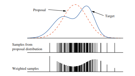
Samples from the proposal distribution are distributed according to $p\left(s^{t}\right.$ $\left.z^{t-1}, u^{t}, n^{t-1}\right)$, and therefore do not match the desired posterior $p\left(s^{t}\right.$ | $\left.z^{t}, u^{t}, n^{t}\right)$. This difference is corrected through importance sampling. An example of importance sampling is shown in Figure 3.6. Instead of sampling directly from the target distribution (shown as a solid line), samples are drawn from a simpler proposal distribution, a Gaussian (shown as a dashed line). In regions where the target distribution is larger than the proposal distribution, the samples receive higher weights. As a result, samples in this region will be picked more often. In regions where the target distribution is smaller than the proposal distribution, the samples will be given lower weights. In the limit of infinite samples, this procedure will produce samples distributed according to the target distribution.
For FastSLAM, the importance weight of each particle $w_{t}^{[i]}$ is equal to the ratio of the SLAM posterior and the proposal distribution described previously.
$$
w_{t}^{[m]}=\frac{\text { target distribution }}{\text { proposal distribution }}=\frac{p\left(s^{t,[m]} \mid z^{t}, u^{t}, n^{t}\right)}{p\left(s^{t,[m]} \mid z^{t-1}, u^{t}, n^{t-1}\right)}
$$
The numerator of (3.37) can be expanded using Bayes Rule. The normalizing constant in Bayes Rule can be safely ignored because the particle weights will be normalized before resampling.
$$
w_{t}^{[m]} \stackrel{\text { Bayes }}{\propto} \frac{p\left(z_{t} \mid s^{t,[m]}, z^{t-1}, u^{t}, n^{t}\right) p\left(s^{t,[m]} \mid z^{t-1}, u^{t}, n^{t}\right)}{p\left(s^{t,[m]} \mid z^{t-1}, u^{t}, n^{t-1}\right)}
$$
The second term of the numerator is not conditioned on the latest observation $z_{t}$, so the data association $n_{t}$ cannot provide any information about the robot’s path. Therefore it can be dropped.
$$
\begin{gathered}
w_{t}^{[m]} \stackrel{\text { Markov }}{=} \frac{p\left(z_{t} \mid s^{t,[m]}, z^{t-1}, u^{t}, n^{t}\right) p\left(s^{t,[m]} \mid z^{t-1}, u^{t}, n^{t-1}\right)}{p\left(s^{t,[m]} \mid z^{t-1}, u^{t}, n^{t-1}\right)} \
=p\left(z_{t} \mid s^{t,[m]}, z^{t-1}, u^{t}, n^{t}\right)
\end{gathered}
$$
The landmark estimator is an EKF, so this observation likelihood can be computed in closed form. This probability is commonly computed in terms of “innovation,” or the difference between the actual observation $z_{t}$ and the predicted observation $\hat{z}{t}$. The sequence of innovations in the EKF is Gaussian with zero mean and covariance $Z{n_{t}, t}$, where $Z_{n_{t}, t}$ is the innovation covariance matrix defined in (3.31) [3]. The probability of the observation $z_{t}$ is equal to the probability of the innovation $z_{t}-\hat{z}{t}$ being generated by this Gaussian, which can be written as: $$ w{t}^{[m]}=\frac{1}{\sqrt{\mid 2 \pi Z_{n_{t}, t}} \mid} \exp \left{-\frac{1}{2}\left(z_{t}-\hat{z}{n{t}, t}\right)^{T}\left[Z_{n_{t}, t}\right]^{-1}\left(z_{t}-\hat{z}{n{t}, t}\right)\right}
$$
Calculating the importance weight is a constant-time operation per particle. This calculation depends only on the dimensionality of the observation, which is constant for a given application.
机器人代写|SLAM代写机器人导航代考|Importance Resampling
Once the temporary particles have been assigned weights, a new set of samples $S_{t}$ is drawn from this set with replacement, with probabilities in proportion to the weights. A variety of sampling techniques for drawing $S_{t}$ can be found in [9]. In particular, Madow’s systematic sampling algorithm [56] is simple to implement and produces accurate results.
Implemented naively, resampling requires time linear in the number of landmarks $N$. This is due to the fact that each particle must be copied to the new particle set, and the length of each particle is proportional to $N$. In general, only a small fraction of the total landmarks will be observed at any one time, so copying the entire particle can be quite inefficient. In Section 3.7, we will show how a more sophisticated particle representation can eliminate unnecessary copying and reduce the computational requirement of FastSLAM to $O(M \log N)$.
At first glace, factoring the SLAM problem using the path of the robot may seem like a bad idea, because the length of the FastSLAM particles will grow over time. However, none of the the FastSLAM update equations depend on the total path length $t$. In fact, only the most recent pose $s_{t-1}^{[m]}$ is used to update the particle set. Consequently, we can silently “forget” all but the most recent robot pose in the parameterization of each particle. This avoids the obvious computational problem that would result if the dimensionality of the particle filter grows over time.
SLAM代写
机器人代写|SLAM代写机器人导航代考|Updating the Landmark Estimates
FastSLAM 表示条件地标估计p(θn∣s吨,和吨,在吨,n吨)在 (3.3) 中使用低维 EKF。现在,我将假设数据关联n吨是已知的。在第 3.4 节中,此限制将被删除。
由于地标估计以机器人的路径为条件,ñEKF 附着在每个粒子上小号吨. 后面超过n-th 地标位置θn很容易获得。它的计算取决于是否n=n吨,即是否有地标θn当时被观察到吨. 对于观察到的地标θn吨,我们遵循使用贝叶斯规则扩展后验的通常程序。
p(θn吨∣s吨,和吨,在吨,n吨)= 贝叶斯 这p(和吨∣θn吨,s吨,和吨−1,在吨,n吨)p(θn吨∣s吨,和吨−1,在吨,n吨)
接下来,马尔可夫属性用于简化方程的两项。观察和吨只取决于θn吨,s吨, 和n吨. 相似地,θn吨不受影响s吨,在吨, 或者n吨没有观察和吨.
p(θn吨∣s吨,和吨,在吨,n吨)= 马尔科夫 这p(和吨∣θn吨,s吨,n吨)p(θn吨∣s吨−1,和吨−1,在吨−1,n吨−1)
为了n≠n吨,我们保持地标后验不变。
p(θn≠n吨∣s吨,和吨,在吨,n吨)=p(θn≠n吨∣s吨−1,和吨−1,在吨−1,n吨−1)
FastSLAM 使用 EKF 实现更新方程(3.22)。与 SLAM 的 EKF 解决方案一样,该滤波器对感知模型使用线性高斯近似。我们注意到,使用实际的线性高斯观测模型,得到的分布p(θn∣s吨,和吨,在吨,n吨)是高斯的,即使运动模型是非线性的。这是对机器人姿势进行采样的结果。
非线性测量模型G(s吨,θn吨)将使用一阶泰勒展开来近似。地标估计器以固定的机器人路径为条件,因此此扩展仅结束θn吨. 我们将假设测量噪声是具有协方差的高斯噪声R吨.
和^吨=G(s吨[米],μn吨,吨−1) Gθn吨=∇θn吨G(s吨,θn吨)|s吨=s吨[米];θn吨=μn吨,吨−1[米] G(s吨,θn吨)≈和^吨+Gθ(θn吨−μn吨,吨−1[米])
在这种近似下,乘积 (3.22) 的第一项分布如下:
p(和吨∣θ一世,s吨,n吨)∼ñ(和吨;和^吨+Gθ(θn吨−μn吨,吨−1[米]),R吨)
机器人代写|SLAM代写机器人导航代考|Calculating Importance Weights
来自提案分布的样本根据p(s吨 和吨−1,在吨,n吨−1),因此不匹配所需的后验p(s吨 | 和吨,在吨,n吨). 这种差异通过重要性抽样得到纠正。图 3.6 显示了一个重要性抽样的例子。样本不是直接从目标分布(显示为实线)中采样,而是从更简单的提议分布中抽取,即高斯分布(显示为虚线)。在目标分布大于提议分布的区域中,样本获得更高的权重。因此,该区域的样本将被更频繁地挑选。在目标分布小于提议分布的区域,样本将被赋予较低的权重。在无限样本的限制下,这个过程会产生按照目标分布分布的样本。
对于 FastSLAM,每个粒子的重要性权重在吨[一世]等于 SLAM 后验与前面描述的提议分布的比率。在吨[米]= 目标分布 提案分发 =p(s吨,[米]∣和吨,在吨,n吨)p(s吨,[米]∣和吨−1,在吨,n吨−1)
(3.37) 的分子可以用贝叶斯法则展开。可以安全地忽略贝叶斯规则中的归一化常数,因为粒子权重将在重采样之前进行归一化。
在吨[米]∝ 贝叶斯 p(和吨∣s吨,[米],和吨−1,在吨,n吨)p(s吨,[米]∣和吨−1,在吨,n吨)p(s吨,[米]∣和吨−1,在吨,n吨−1)
分子的第二项不以最新观察为条件和吨,所以数据关联n吨无法提供有关机器人路径的任何信息。因此它可以被丢弃。
在吨[米]= 马尔科夫 p(和吨∣s吨,[米],和吨−1,在吨,n吨)p(s吨,[米]∣和吨−1,在吨,n吨−1)p(s吨,[米]∣和吨−1,在吨,n吨−1) =p(和吨∣s吨,[米],和吨−1,在吨,n吨)
地标估计器是 EKF,因此可以以封闭形式计算这种观察可能性。该概率通常根据“创新”或实际观察结果之间的差异来计算和吨和预测的观察和^吨. EKF 中的创新序列是具有零均值和协方差的高斯序列从n吨,吨, 在哪里从n吨,吨是 (3.31) [3] 中定义的创新协方差矩阵。观察的概率和吨等于创新的概率和吨−和^吨由这个高斯生成,可以写成:w{t}^{[m]}=\frac{1}{\sqrt{\mid 2 \pi Z_{n_{t}, t}} \mid} \exp \left{-\frac{1}{ 2}\left(z_{t}-\hat{z}{n{t}, t}\right)^{T}\left[Z_{n_{t}, t}\right]^{-1} \left(z_{t}-\hat{z}{n{t}, t}\right)\right}w{t}^{[m]}=\frac{1}{\sqrt{\mid 2 \pi Z_{n_{t}, t}} \mid} \exp \left{-\frac{1}{ 2}\left(z_{t}-\hat{z}{n{t}, t}\right)^{T}\left[Z_{n_{t}, t}\right]^{-1} \left(z_{t}-\hat{z}{n{t}, t}\right)\right}
计算重要性权重是每个粒子的恒定时间操作。此计算仅取决于观察的维度,对于给定的应用程序而言,该维度是恒定的。
机器人代写|SLAM代写机器人导航代考|Importance Resampling
一旦临时粒子被分配了权重,一组新的样本小号吨是从这个集合中抽取的,有放回,概率与权重成正比。绘图的多种采样技术小号吨可以在[9]中找到。特别是,Madow 的系统采样算法 [56] 易于实现并产生准确的结果。
天真地实施,重采样需要与地标数量成线性关系的时间ñ. 这是因为每个粒子都必须复制到新的粒子集,并且每个粒子的长度与ñ. 通常,在任何时候都只会观察到总界标的一小部分,因此复制整个粒子的效率可能非常低。在第 3.7 节中,我们将展示更复杂的粒子表示如何消除不必要的复制并将 FastSLAM 的计算要求降低到这(米日志ñ).
乍一看,使用机器人的路径来分解 SLAM 问题似乎是个坏主意,因为 FastSLAM 粒子的长度会随着时间的推移而增长。然而,FastSLAM 更新方程都不依赖于总路径长度吨. 事实上,只有最近的姿势s吨−1[米]用于更新粒子集。因此,我们可以在每个粒子的参数化中默默地“忘记”除了最近的机器人姿势之外的所有姿势。这避免了如果粒子滤波器的维数随时间增长而导致的明显计算问题。

统计代写请认准statistics-lab™. statistics-lab™为您的留学生涯保驾护航。
金融工程代写
金融工程是使用数学技术来解决金融问题。金融工程使用计算机科学、统计学、经济学和应用数学领域的工具和知识来解决当前的金融问题,以及设计新的和创新的金融产品。
非参数统计代写
非参数统计指的是一种统计方法,其中不假设数据来自于由少数参数决定的规定模型;这种模型的例子包括正态分布模型和线性回归模型。
广义线性模型代考
广义线性模型(GLM)归属统计学领域,是一种应用灵活的线性回归模型。该模型允许因变量的偏差分布有除了正态分布之外的其它分布。
术语 广义线性模型(GLM)通常是指给定连续和/或分类预测因素的连续响应变量的常规线性回归模型。它包括多元线性回归,以及方差分析和方差分析(仅含固定效应)。
有限元方法代写
有限元方法(FEM)是一种流行的方法,用于数值解决工程和数学建模中出现的微分方程。典型的问题领域包括结构分析、传热、流体流动、质量运输和电磁势等传统领域。
有限元是一种通用的数值方法,用于解决两个或三个空间变量的偏微分方程(即一些边界值问题)。为了解决一个问题,有限元将一个大系统细分为更小、更简单的部分,称为有限元。这是通过在空间维度上的特定空间离散化来实现的,它是通过构建对象的网格来实现的:用于求解的数值域,它有有限数量的点。边界值问题的有限元方法表述最终导致一个代数方程组。该方法在域上对未知函数进行逼近。[1] 然后将模拟这些有限元的简单方程组合成一个更大的方程系统,以模拟整个问题。然后,有限元通过变化微积分使相关的误差函数最小化来逼近一个解决方案。
tatistics-lab作为专业的留学生服务机构,多年来已为美国、英国、加拿大、澳洲等留学热门地的学生提供专业的学术服务,包括但不限于Essay代写,Assignment代写,Dissertation代写,Report代写,小组作业代写,Proposal代写,Paper代写,Presentation代写,计算机作业代写,论文修改和润色,网课代做,exam代考等等。写作范围涵盖高中,本科,研究生等海外留学全阶段,辐射金融,经济学,会计学,审计学,管理学等全球99%专业科目。写作团队既有专业英语母语作者,也有海外名校硕博留学生,每位写作老师都拥有过硬的语言能力,专业的学科背景和学术写作经验。我们承诺100%原创,100%专业,100%准时,100%满意。
随机分析代写
随机微积分是数学的一个分支,对随机过程进行操作。它允许为随机过程的积分定义一个关于随机过程的一致的积分理论。这个领域是由日本数学家伊藤清在第二次世界大战期间创建并开始的。
时间序列分析代写
随机过程,是依赖于参数的一组随机变量的全体,参数通常是时间。 随机变量是随机现象的数量表现,其时间序列是一组按照时间发生先后顺序进行排列的数据点序列。通常一组时间序列的时间间隔为一恒定值(如1秒,5分钟,12小时,7天,1年),因此时间序列可以作为离散时间数据进行分析处理。研究时间序列数据的意义在于现实中,往往需要研究某个事物其随时间发展变化的规律。这就需要通过研究该事物过去发展的历史记录,以得到其自身发展的规律。
回归分析代写
多元回归分析渐进(Multiple Regression Analysis Asymptotics)属于计量经济学领域,主要是一种数学上的统计分析方法,可以分析复杂情况下各影响因素的数学关系,在自然科学、社会和经济学等多个领域内应用广泛。
MATLAB代写
MATLAB 是一种用于技术计算的高性能语言。它将计算、可视化和编程集成在一个易于使用的环境中,其中问题和解决方案以熟悉的数学符号表示。典型用途包括:数学和计算算法开发建模、仿真和原型制作数据分析、探索和可视化科学和工程图形应用程序开发,包括图形用户界面构建MATLAB 是一个交互式系统,其基本数据元素是一个不需要维度的数组。这使您可以解决许多技术计算问题,尤其是那些具有矩阵和向量公式的问题,而只需用 C 或 Fortran 等标量非交互式语言编写程序所需的时间的一小部分。MATLAB 名称代表矩阵实验室。MATLAB 最初的编写目的是提供对由 LINPACK 和 EISPACK 项目开发的矩阵软件的轻松访问,这两个项目共同代表了矩阵计算软件的最新技术。MATLAB 经过多年的发展,得到了许多用户的投入。在大学环境中,它是数学、工程和科学入门和高级课程的标准教学工具。在工业领域,MATLAB 是高效研究、开发和分析的首选工具。MATLAB 具有一系列称为工具箱的特定于应用程序的解决方案。对于大多数 MATLAB 用户来说非常重要,工具箱允许您学习和应用专业技术。工具箱是 MATLAB 函数(M 文件)的综合集合,可扩展 MATLAB 环境以解决特定类别的问题。可用工具箱的领域包括信号处理、控制系统、神经网络、模糊逻辑、小波、仿真等。