如果你也在 怎样代写电动力学electrodynamics这个学科遇到相关的难题,请随时右上角联系我们的24/7代写客服。
电动力学是物理学的一个分支,处理快速变化的电场和磁场。
statistics-lab™ 为您的留学生涯保驾护航 在代写电动力学electrodynamics方面已经树立了自己的口碑, 保证靠谱, 高质且原创的统计Statistics代写服务。我们的专家在代写电动力学electrodynamics代写方面经验极为丰富,各种代写电动力学electrodynamics相关的作业也就用不着说。
我们提供的电动力学electrodynamics及其相关学科的代写,服务范围广, 其中包括但不限于:
- Statistical Inference 统计推断
- Statistical Computing 统计计算
- Advanced Probability Theory 高等概率论
- Advanced Mathematical Statistics 高等数理统计学
- (Generalized) Linear Models 广义线性模型
- Statistical Machine Learning 统计机器学习
- Longitudinal Data Analysis 纵向数据分析
- Foundations of Data Science 数据科学基础
物理代写|电动力学代写electromagnetism代考|Review of Brownian Probability
About half of [MTRV] is taken up with $(5.8),(5.12)$, and related expressions. When motivational and explanatory material is included, these expressions, along with their properties and implications, constitute almost all of the present
book whenever the Feynman quantum mechanical expression (8.29) of Section $8.6$ below is included.
[MTRV] uses the symbol $\mathcal{G}$ for geometric Brownian distribution function (5.12). while the symbol $G_{c}(I[N])$ is used to denote the joint distribution function for $c$-Brownian motion. So $G_{-\frac{1}{2}}$ gives standard or classical Brownian motion (5.8); while $G_{\frac{1}{2}}$ is used in [MTRV] for the Feynman theory of (8.29).
But in this book the symbol $G$ is used without subscript, allowing the context (Brownian motion or quantum mechanics) to show which meaning is intended.
To sum up, the theory of $(5.8),(5.12)$, and $(8.29)$ is covered in chapters 6,7 , and 8 of [MTRV]. It is not proposed to rehearse this theory here; but, instead, to highlight some aspects of it which are particularly relevant to the topics of this book.
In [MTRV], Brownian motion, geometric Brownian motion, and Feynman path integration (for single particle mechanical phenomena) are united in a single theory based on a version of Fresnel’s integral using a parameter $c=a+\iota b$, where $\iota=\sqrt{-1}, a \leq 0$, and $c \neq 0$ (so $a$ and $b$ are not both zero.)
The case $c=-\frac{1}{2}$ (real, negative) leads to Brownian and geometric Brownian motion. The case $c=\frac{\sqrt{-1}}{2}$ (pure imaginary) gives Feynman path integrals. The designation $c$-Brownian motion is intended to cover all cases, including those which are “intermediate” between real negative and pure imaginary.
The Fresnel evaluation is in theorem 133 (pages 261-262 of [MTRV]). For $c<0$ (real, negative) lemmas 12 and 13 (page 262) show that finite compositions (or addition) of normal distributions are normal, so that these distributions are additive in some sense. And provided the real part of $c$ is non-positive (with $c \neq 0$ ), lemmas 12 and 13 are valid for complex-valued $c$.
These results are crucial in going from finite compositions of distributions to infinite compositions, giving a theory of infinitely many (and “infinitely divisible” ${ }^{n}$ or continuum) of normal distributions (or c-normal distributions), leading to the theory of $c$-Brownian motion.
Joint probability distributions are defined on domains $\mathbf{R}^{\mathbf{T}}$ where $\mathbf{T}$ is typically a real interval open on the left and closed on the right, such as
$$
] 0, t], \quad] 0, \tau], \quad] \tau^{\prime}, \tau\right] \text {. }
$$
A joint distribution such as $(5.8),(5.12)$, or $(8.29)$, is constructed for samples
$$
N=\left{t_{1}, t_{2}, \ldots, t_{n-1}, t_{n}\right} \subset \mathbf{T}
$$
with $t_{0}$ taken to be the left hand boundary of interval $\mathbf{T}$, and $t_{n}$ the right hand boundary point.
物理代写|电动力学代写electromagnetism代考|Brownian Stochastic Integration
A stochastic integral with respect to Brownian processes can have forms
$$
\int_{0}^{t} g(s) d X(s), \quad \int_{0}^{t} f(X(s)) d X(s), \quad \int_{0}^{t} Z(s) d X(s) .
$$
Each random variable $X(s)(0<s \leq t)$ is normally distributed, so individually they are not too difficult.
But $\int_{0}^{t}$ involves a continuum of such normal distributions. Section $4.4$ mentions step functions, cylinder functions, and sampling functions as a progression of stages in dealing with this problem. This section applies a cylinder function approach to Brownian stochastic integrals. The idea is to replace the continuum ] $0, t]$ by discrete times $0=\tau_{0}<\tau_{1}<\cdots<\tau_{n}=t$. (In Part II, R. Feynman’s path integrals of cylinder functions use a countable infinity of discrete times $\tau_{j}$-)
For $0<t \leq \tau$ let $\mathbf{T}$ denote $] 0, t]$, closed at boundary $t$; and let $T$ denote $] 0, t[$, open at boundary $t$. Suppose an asset price process $X_{T}$ can be represented as
$$
X_{\mathrm{T}} \simeq x_{\mathrm{T}}\left[\mathbf{R}^{\mathbf{T}}, G\right]
$$
where $x(0)=0$ for all sample paths, and $G$ is the joint probability distribution function $G(I[N])$ of $(5.8)$ for standard Brownian motion. Assume the asset is some portfolio which (unlike shares) can take unbounded positive and negative values. In other words the “asset” (or portfolio) can also be a liability.
A distinction can be made between the value of the portfolio at any time $t$, and the earnings of the portfolio at time $t$.
The latter is intended to denote the stake of the investor or holder of the portfolio, taking account of the initial expenditure (denoted below by $\beta$ ) paid out by the investor in order to acquire possession of the portfolio to begin with.
The former represents a third party view of the portfolio, disregarding any cost of acquisition. If $w(t)$ is the value of the portfolio then earnings equal $w(t)-\beta$ for all $t$; where $\beta$ denotes the upfront cost to the investor of acquiring the portfolio at time $t=0$.
The value of the portfolio at any time $s$ depends on the size $\nu(s)$ of (or number of units of the assets/liabilities in) the portfolio. Then the value of the portfolio at time $s$ is $\nu(s) x(s)$. For the purpose of investigating stochastic integrals, the number $\nu(s)$ can have various interpretations, such as
$$
g(s), \quad Z(s), \quad f(X(s))
$$
where, for $0 \leq s \leq t, g(s)$ is a deterministic 4 function, $(Z(s))$ is a random process independent of the Brownian motion $(X(s))$, and $(f(X(s)))$ is a process which depends on $(X(s))$.
物理代写|电动力学代写electromagnetism代考|Some Features of Brownian Motion
Example 19 above suggests there is a need to consider some extreme behaviour of Brownian paths.
Mathematical Brownian motion is very “bad”. A stereotypical pictorial representation of a sample element of Brownian motion is a “jagged-path” graph consisting of straight line segments adjoining each other consecutively with sharp corners at the points where each one adjoins the next one.
Mathematically, however, a typical sample path is nowhere differentiable. This is much “worse” than the jagged-path graphical representation. Except for their end points, line segments are smooth, or differentiable. So the class of all such jagged paths are a $G$-null subset of the sample space $\Omega=\mathbf{R}^{\mathbf{T}}$.
The reason for this “badness” is that, typically, the increments or transitions $x\left(s^{\prime}\right)-x(s)$ vary as the square root of the time increment $s^{\prime}-s$. Calculating a derivative for $x(s)$ at $s$ involves
$$
\frac{x\left(s^{\prime}\right)-x(s)}{s^{\prime}-s}=\frac{1}{\sqrt{s^{\prime}-s}}\left(\frac{x\left(s^{\prime}\right)-x(s)}{\sqrt{s^{\prime}-s}}\right)
$$
which diverges as $s^{\prime} \rightarrow s$ for “typical” $x$ of Brownian motion, since the final factor remains finite for such $x$.
From a different perspective, mathematical Brownian motion is very “good”. This is because, typically ${ }^{10}$, its sample paths are uniformly continuous. The reason for this “goodness” is that, typically, the increments or transitions $x\left(s^{\prime}\right)$ $x(s)$ vary as the square root of the time increment $s^{\prime}-s$. So if $s^{\prime} \rightarrow s$ then $\sqrt{s^{\prime}-s} \rightarrow 0$ and hence $x\left(s^{\prime}\right) \rightarrow x(s) .$
These issues are discussed in detail in chapter 6 of [MTRV], and in many other presentations of the subject
Brownian motion includes sample paths which resemble the Dirichlet function of Example 13, and it includes straight lines, and it includes everything in between these two extremes.
In this book stochastic integrals have been presented as some kind of Stieltjes integral, involving integration of one point function $h_{1}(s)$ with respect to a different point function $h_{2}(s)$. (In Section $5.4$ the integrator function $h_{2}\left(s^{\prime}\right)$ $h_{2}(s)$ was supposed to be a Brownian sample path increment $x\left(s^{\prime}\right)-x(s)$; while the integrand function $h_{1}(s)$ was generally designated as $g(s)$.)
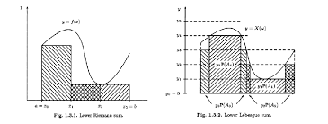
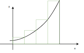
A basic Riemann-Stieltjes integral has Riemann sum approximations of the form
$$
\sum h_{1}\left(s^{\prime \prime}\right)\left(h_{2}\left(s^{\prime}\right)-h_{2}(s)\right)
$$
where $s^{\prime \prime}$ satisfies $s \leq s^{\prime \prime} \leq s^{\prime}$; so $s^{\prime \prime}$ could be taken to be $s$ for every term of the Riemann sum. This fits in with the usual form of the stochastic integral (notably in finance) where $s^{\prime \prime}$ is taken to be the initial $s$ of the time increment $\left[s, s^{\prime}[\right.$.
电动力学代考
物理代写|电动力学代写electromagnetism代考|Review of Brownian Probability
大约一半的 [MTRV] 被占用(5.8),(5.12),以及相关的表达方式。当包含激励性和解释性材料时,这些表达以及它们的属性和含义几乎构成了当前的所有内容
书每当费曼量子力学表达式(8.29)的第8.6以下包括在内。
[MTRV] 使用符号G对于几何布朗分布函数(5.12)。而符号GC(我[ñ])用于表示联合分布函数C-布朗运动。所以G−12给出标准或经典布朗运动 (5.8);尽管G12在 [MTRV] 中用于 (8.29) 的费曼理论。
但在这本书中,符号G不带下标使用,允许上下文(布朗运动或量子力学)显示预期的含义。
综上所述,理论(5.8),(5.12), 和(8.29)在 [MTRV] 的第 6,7 和 8 章中进行了介绍。不建议在这里排练这个理论;而是强调它的某些方面,这些方面与本书的主题特别相关。
在 [MTRV] 中,布朗运动、几何布朗运动和费曼路径积分(用于单粒子力学现象)结合在一个单一的理论中,该理论基于使用参数的菲涅耳积分版本C=一个+我b, 在哪里我=−1,一个≤0, 和C≠0(所以一个和b不都是零。)
案子C=−12(实数,负数)导致布朗运动和几何布朗运动。案子C=−12(纯虚数)给出费曼路径积分。指定C-布朗运动旨在涵盖所有情况,包括那些介于真实否定和纯想象之间的“中间”。
菲涅耳评估在定理 133 中([MTRV] 第 261-262 页)。为了C<0(实数,负数)引理 12 和 13(第 262 页)表明正态分布的有限组合(或加法)是正态的,因此这些分布在某种意义上是相加的。并提供了真实的部分C是非正数(与C≠0),引理 12 和 13 对复值有效C.
这些结果对于从分布的有限组合到无限组合至关重要,给出了无限多(和“无限可分”的理论)n或连续体)的正态分布(或 c-正态分布),导致理论C-布朗运动。
联合概率分布在域上定义R吨在哪里吨通常是左开右闭的实区间,例如
] 0, t], \quad] 0, \tau], \quad] \tau^{\prime}, \tau\right] \text {. }] 0, t], \quad] 0, \tau], \quad] \tau^{\prime}, \tau\right] \text {. }
联合分布,例如(5.8),(5.12), 或者(8.29), 是为样本构建的
N=\left{t_{1}, t_{2}, \ldots, t_{n-1}, t_{n}\right} \subset \mathbf{T}N=\left{t_{1}, t_{2}, \ldots, t_{n-1}, t_{n}\right} \subset \mathbf{T}
和吨0取为区间的左边界吨, 和吨n右手边的边界点。
物理代写|电动力学代写electromagnetism代考|Brownian Stochastic Integration
关于布朗过程的随机积分可以有形式
∫0吨G(s)dX(s),∫0吨F(X(s))dX(s),∫0吨从(s)dX(s).
每个随机变量X(s)(0<s≤吨)是正态分布的,所以单独它们并不太难。
但∫0吨涉及这种正态分布的连续统一体。部分4.4提到阶跃函数、圆柱函数和采样函数作为处理这个问题的一个阶段的进展。本节将圆柱函数方法应用于布朗随机积分。这个想法是替换连续体]0,吨]按离散时间0=τ0<τ1<⋯<τn=吨. (在第二部分中,R. Feynman 的柱面函数路径积分使用可数无穷大的离散时间τj-)
对于0<吨≤τ让吨表示]0,吨], 在边界处闭合吨; 然后让吨表示]0,吨[, 在边界处打开吨. 假设一个资产价格过程X吨可以表示为
X吨≃X吨[R吨,G]
在哪里X(0)=0对于所有样本路径,以及G是联合概率分布函数G(我[ñ])的(5.8)对于标准布朗运动。假设资产是一些(与股票不同)可以取无限正负值的投资组合。换句话说,“资产”(或投资组合)也可以是负债。
可以随时区分投资组合的价值吨,以及当时投资组合的收益吨.
后者旨在表示投资者或投资组合持有人的股份,考虑到初始支出(以下表示为b) 由投资者支付,以便一开始就获得投资组合的所有权。
前者代表投资组合的第三方观点,不考虑任何收购成本。如果在(吨)是投资组合的价值然后收益相等在(吨)−b对所有人吨; 在哪里b表示投资者当时获得投资组合的前期成本吨=0.
任何时候投资组合的价值s取决于大小ν(s)投资组合的数量(或资产/负债的单位数量)。那么投资组合在时间的价值s是ν(s)X(s). 为了研究随机积分,数ν(s)可以有多种解释,例如
G(s),从(s),F(X(s))
其中,对于0≤s≤吨,G(s)是确定性 4 函数,(从(s))是一个独立于布朗运动的随机过程(X(s)), 和(F(X(s)))是一个依赖于的过程(X(s)).
物理代写|电动力学代写electromagnetism代考|Some Features of Brownian Motion
上面的示例 19 表明有必要考虑布朗路径的一些极端行为。
数学布朗运动非常“糟糕”。布朗运动样本元素的典型图形表示是一个“锯齿状路径”图,由彼此连续相邻的直线段组成,每个直线段与下一个直线段相邻的点处有尖角。
然而,从数学上讲,典型的样本路径是无处可微的。这比锯齿状路径图形表示“糟糕”得多。除了端点之外,线段是平滑的或可微分的。所以所有这些锯齿状路径的类都是G- 样本空间的空子集Ω=R吨.
这种“坏事”的原因是,通常情况下,增量或过渡X(s′)−X(s)随时间增量的平方根而变化s′−s. 计算导数X(s)在s涉及
X(s′)−X(s)s′−s=1s′−s(X(s′)−X(s)s′−s)
它发散为s′→s对于“典型”X布朗运动的,因为对于这样的最终因素仍然是有限的X.
从不同的角度来看,数学布朗运动非常“好”。这是因为,通常10,其样本路径是一致连续的。这种“好”的原因是,通常,增量或过渡X(s′) X(s)随时间增量的平方根而变化s′−s. 因此,如果s′→s然后s′−s→0因此X(s′)→X(s).
[MTRV] 的第 6 章以及该主题的许多其他介绍中详细讨论了这些问题
布朗运动包括类似于示例 13 的狄利克雷函数的样本路径,它包括直线,它包括这两个极端之间的所有内容。
在本书中,随机积分被描述为某种 Stieltjes 积分,涉及单点函数的积分H1(s)关于不同的点函数H2(s). (在部分5.4积分器功能H2(s′) H2(s)应该是布朗样本路径增量X(s′)−X(s); 而被积函数H1(s)一般被指定为G(s).)
一个基本的 Riemann-Stieltjes 积分具有以下形式的 Riemann 和近似值
∑H1(s′′)(H2(s′)−H2(s))
在哪里s′′满足s≤s′′≤s′; 所以s′′可以认为是s对于黎曼和的每一项。这符合随机积分的通常形式(尤其是在金融领域),其中s′′被认为是初始的s时间增量[s,s′[.

统计代写请认准statistics-lab™. statistics-lab™为您的留学生涯保驾护航。
金融工程代写
金融工程是使用数学技术来解决金融问题。金融工程使用计算机科学、统计学、经济学和应用数学领域的工具和知识来解决当前的金融问题,以及设计新的和创新的金融产品。
非参数统计代写
非参数统计指的是一种统计方法,其中不假设数据来自于由少数参数决定的规定模型;这种模型的例子包括正态分布模型和线性回归模型。
广义线性模型代考
广义线性模型(GLM)归属统计学领域,是一种应用灵活的线性回归模型。该模型允许因变量的偏差分布有除了正态分布之外的其它分布。
术语 广义线性模型(GLM)通常是指给定连续和/或分类预测因素的连续响应变量的常规线性回归模型。它包括多元线性回归,以及方差分析和方差分析(仅含固定效应)。
有限元方法代写
有限元方法(FEM)是一种流行的方法,用于数值解决工程和数学建模中出现的微分方程。典型的问题领域包括结构分析、传热、流体流动、质量运输和电磁势等传统领域。
有限元是一种通用的数值方法,用于解决两个或三个空间变量的偏微分方程(即一些边界值问题)。为了解决一个问题,有限元将一个大系统细分为更小、更简单的部分,称为有限元。这是通过在空间维度上的特定空间离散化来实现的,它是通过构建对象的网格来实现的:用于求解的数值域,它有有限数量的点。边界值问题的有限元方法表述最终导致一个代数方程组。该方法在域上对未知函数进行逼近。[1] 然后将模拟这些有限元的简单方程组合成一个更大的方程系统,以模拟整个问题。然后,有限元通过变化微积分使相关的误差函数最小化来逼近一个解决方案。
tatistics-lab作为专业的留学生服务机构,多年来已为美国、英国、加拿大、澳洲等留学热门地的学生提供专业的学术服务,包括但不限于Essay代写,Assignment代写,Dissertation代写,Report代写,小组作业代写,Proposal代写,Paper代写,Presentation代写,计算机作业代写,论文修改和润色,网课代做,exam代考等等。写作范围涵盖高中,本科,研究生等海外留学全阶段,辐射金融,经济学,会计学,审计学,管理学等全球99%专业科目。写作团队既有专业英语母语作者,也有海外名校硕博留学生,每位写作老师都拥有过硬的语言能力,专业的学科背景和学术写作经验。我们承诺100%原创,100%专业,100%准时,100%满意。
随机分析代写
随机微积分是数学的一个分支,对随机过程进行操作。它允许为随机过程的积分定义一个关于随机过程的一致的积分理论。这个领域是由日本数学家伊藤清在第二次世界大战期间创建并开始的。
时间序列分析代写
随机过程,是依赖于参数的一组随机变量的全体,参数通常是时间。 随机变量是随机现象的数量表现,其时间序列是一组按照时间发生先后顺序进行排列的数据点序列。通常一组时间序列的时间间隔为一恒定值(如1秒,5分钟,12小时,7天,1年),因此时间序列可以作为离散时间数据进行分析处理。研究时间序列数据的意义在于现实中,往往需要研究某个事物其随时间发展变化的规律。这就需要通过研究该事物过去发展的历史记录,以得到其自身发展的规律。
回归分析代写
多元回归分析渐进(Multiple Regression Analysis Asymptotics)属于计量经济学领域,主要是一种数学上的统计分析方法,可以分析复杂情况下各影响因素的数学关系,在自然科学、社会和经济学等多个领域内应用广泛。
MATLAB代写
MATLAB 是一种用于技术计算的高性能语言。它将计算、可视化和编程集成在一个易于使用的环境中,其中问题和解决方案以熟悉的数学符号表示。典型用途包括:数学和计算算法开发建模、仿真和原型制作数据分析、探索和可视化科学和工程图形应用程序开发,包括图形用户界面构建MATLAB 是一个交互式系统,其基本数据元素是一个不需要维度的数组。这使您可以解决许多技术计算问题,尤其是那些具有矩阵和向量公式的问题,而只需用 C 或 Fortran 等标量非交互式语言编写程序所需的时间的一小部分。MATLAB 名称代表矩阵实验室。MATLAB 最初的编写目的是提供对由 LINPACK 和 EISPACK 项目开发的矩阵软件的轻松访问,这两个项目共同代表了矩阵计算软件的最新技术。MATLAB 经过多年的发展,得到了许多用户的投入。在大学环境中,它是数学、工程和科学入门和高级课程的标准教学工具。在工业领域,MATLAB 是高效研究、开发和分析的首选工具。MATLAB 具有一系列称为工具箱的特定于应用程序的解决方案。对于大多数 MATLAB 用户来说非常重要,工具箱允许您学习和应用专业技术。工具箱是 MATLAB 函数(M 文件)的综合集合,可扩展 MATLAB 环境以解决特定类别的问题。可用工具箱的领域包括信号处理、控制系统、神经网络、模糊逻辑、小波、仿真等。