如果你也在 怎样代写工程统计Engineering Statistics这个学科遇到相关的难题,请随时右上角联系我们的24/7代写客服。
工程统计结合了工程和统计,使用科学方法分析数据。工程统计涉及有关制造过程的数据,如:部件尺寸、公差、材料类型和制造过程控制。
statistics-lab™ 为您的留学生涯保驾护航 在代写工程统计Engineering Statistics方面已经树立了自己的口碑, 保证靠谱, 高质且原创的统计Statistics代写服务。我们的专家在代写工程统计Engineering Statistics代写方面经验极为丰富,各种代写工程统计Engineering Statistics相关的作业也就用不着说。
我们提供的工程统计Engineering Statistics及其相关学科的代写,服务范围广, 其中包括但不限于:
- Statistical Inference 统计推断
- Statistical Computing 统计计算
- Advanced Probability Theory 高等概率论
- Advanced Mathematical Statistics 高等数理统计学
- (Generalized) Linear Models 广义线性模型
- Statistical Machine Learning 统计机器学习
- Longitudinal Data Analysis 纵向数据分析
- Foundations of Data Science 数据科学基础
统计代写|工程统计作业代写Engineering Statistics代考|Discrete Distributions
There are two classes of distributions: Discrete and continuous. Discrete distributions are used to describe data that can have only discrete values. Such data have a specific probability associated with each value of the random variable. There are distinct and measurable step changes associated with each value of the variable. Some examples of discrete variables are the size of the last raise you received (it was not in fractions of a cent), the score of the last sporting event you watched, the number of personal protective equipment items available to you on your job, the number of first-quality computer chips on a silicon wafer, the number of defects in a skein of yarn, the energy of electrons in a particular quantum state, the number of raindrops that fall onto a square inch of land, etc.
The variable $x_{i}$ represents the count of events in the $i$ th category. The categories are mutually exclusive, such as alphabet letters, or pass/fail. The value of $x_{i}$ is an integer number. Looking at this paragraph, if $I=1$ represents the occurrence of the letter “a” and $I=2$ that of the letter ” $\mathrm{b}$ “, then the value of $x_{1}=18$ and $x_{2}=4$.
Probability density functions, $p d f\left(x_{i}\right)$ or simply $f\left(x_{i}\right)$, are associated with distributions of discrete variables, $x_{i}$ represent the probability of possible values of the ith data category. For example, if you flip a coin you expect $k=2$, two outcomes, Head and Tail, or 0 and 1 . If the first classification of $x_{1}=$ Head, then $f\left(x_{1}\right)=0.5$. All such probability functions have the following properties:
- $x_{i}$ are the discrete possible values of a variable $X$, and $x_{\mathrm{i}}$ is the $i$ th of the $k$ finite values of the outcome. Usually, the index $i$ places the $x_{i}$ values in ascending order.
- The probability functions are mathematical models of the population, of the infinity of possible samples, not of a finite sample of $k$ number of values.
- $f\left(x_{i}\right)$ is the frequency, the probability of occurrence that a value $x_{i}$ will occur. It is positive and real for each $x_{\dot{r}} f\left(x_{i}\right)=\lim {n \rightarrow \infty}\left{n{i} / n\right}$.
- $\sum_{i=1}^{k} f\left(x_{i}\right)=1$ where $k$ is the number of categories.
- $P(E)=\sum f\left(x_{i}\right)$ where the sum includes all $x_{i}$ in the event $E$.
These definitions illustrate the notation we use throughout this book. We use capital Latin letters for populations and lowercase Latin letters for particular numerical observation values from the populations. Lowercase Greek letters are used for population parameters. Point and cumulative distributions are identified by $f$ and $F$ (or alternately CDF) respectively. $P$ stands for “probability of …”. We are using the conventional notation for discrete distributions: $x$ in the summations of the cumulative distribution functions of discrete distributions sometimes represents the number of items in a class (group, collection, etc.) or at other times, $x$ represents the numerical value that quantifies the class. By using this notation, the formulas in this book are consistent with those you may find in other statistics books. We state this as a warning, because in conventional notation for variables, $x$ means the value of the variable as opposed to the number of occurrences in a category. The cumulative distribution function (CDF) is a function $F\left(x_{n}\right)$ obtained from the probability function and is defined for the values of $x_{i}$ of the random variable $X$ by
$$
F\left(x_{r}\right)=F\left(x_{r}\right)=P\left(X \leq x_{r}\right)= \begin{cases}0 & \text { for } X<x_{1} \ \sum_{i=1}^{r} f\left(x_{i}\right) & \text { where } x_{1} \leq X \leq x \ 1 & \text { for } X \geq x_{n}\end{cases}
$$
统计代写|工程统计作业代写Engineering Statistics代考|Discrete Uniform Distribution
When each discrete event has the same likelihood (probability) of occurring, the probability function is given by
$$
f\left(x_{i}\right)=\frac{1}{n}, \quad 1 \leq i<n
$$
where $n$ is the number of discrete values for $x$. For the cumulative discrete distribution function,
$$
F\left(x_{i}\right)=P\left(X \leq x_{i}\right)=\frac{i}{n}
$$
where $x_{1}<x_{2}<x_{3} \ldots<x_{n}$
A classic example is that of rolling a cubical die. The $n=6$ categories of possible outcomes are equally probable.
The $X$ in Equation (3.6) may represent either a dimensionless counting number ( 7 bolts), a category ( 3 Heads) or a dimensional real number (last raise was $\$ 437.25 / \mathrm{month}$ ); however, $X$ must be limited to a finite number, $n$, of discrete values. For the raise example, the discrete values are multiples of $1 \mathrm{c} / \mathrm{month}$. If the maximum possible raise could have been $\$ 600.00 /$ month, then $n=600.00 / .01+1=60,001$ (we cannot exclude the zero-raise event). Consequently, $x_{10,000}$ represents the 10,000 th value of $X$, which is $\$ 99.99 / \mathrm{mon}$ th.
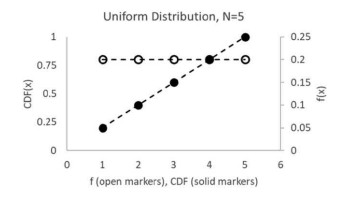
Figure $3.1$ illustrates the discrete uniform distribution for $n=5$, and the corresponding cumulative discrete uniform distribution, also for $n=5$.
Recognizing that each $x_{i}$ value has the same probability, or frequency of occurring, $f\left(x_{i}\right)=f\left(x_{j}\right)$, the mean and variance of the discrete uniform distribution are
$$
\begin{gathered}
\mu=\frac{1}{n} \sum_{i=1}^{n} x_{i} \
\sigma^{2}=\frac{1}{n} \sum_{i=1}^{n}\left(x_{i}-\mu\right)^{2}
\end{gathered}
$$
If the $x_{i}$ values are also equally incremented between $x_{1}=a$ and $x_{n}=b$, so that $x_{j+1}-x_{j}=$ $\Delta x=(b-a) / n$ (such as with a die which has sides with values of $1,2,3 \ldots, 6$, where $a=1$ and $b=6$ ) then
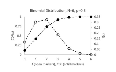
统计代写|工程统计作业代写Engineering Statistics代考|Binomial Distribution
A discrete distribution called the binomial occurs when any observation can be placed in only one of two mutually exclusive categories, such as greater-than or less-than-or-equalto, safe or unsafe, hot or cold, on or off, 0 or 1, pass or fail, Heads or Tails, etc. Although these characteristics are qualitative, the distribution can be made quantitative by assigning the values 0 and 1 to the two categories. The method of assignment is immaterial so long as it is consistent. Customarily, the categories are labeled success (value $=1$ ) and
failure (value $=0$ ). If $p=$ probability of success and $q=1-p=$ probability of failure in one trial of the experiment (one observation), the probability of exactly $x$ number of successes in $n$ trials can be described by the corresponding term of the binomial expansion, or
$$
f(x \mid n)=\left(\begin{array}{l}
n \
x
\end{array}\right) p^{x} q^{n-x} \equiv \frac{n !}{x !(n-x) !} p^{x} q^{n-x}, x=0,1,2, \ldots, n
$$
where $X$ may only have integer values.
Note: The $\left(\begin{array}{l}n \ x\end{array}\right)$ symbol does not mean $n$ divided by $x$, it represents $\frac{n !}{x !(n-x) !}$, which is the number of combinations (ways) of having $x$ occur in $n$ trials. If $n=4$ and $x=2$ then $\left(\begin{array}{l}n \ x\end{array}\right)=\frac{4 !}{2 !(4-2) !}=\frac{4 \times 3 \times 2 \times 1}{2 \times 1(2 \times 1)}=6$. The six possible success-fail patterns could be 1100,1010 , 1001, 0110, 0101, and $0011 .$
Note: The variable $x$ represents the numerical count in a particular category, it is not the value of the category.
Note: When $n$ is large, the factorial terms become large, and direct calculation of either the numerator or denominator can result in digital overflow. Fortunately, the number of integers in the numerator and denominator is equal, there are $n$ digits in each, and a best way to calculate the ratio is to alternate dividing and multiplying. But, many software packages provide convenient functions. In Excel the function is $f(x \mid n)=\operatorname{BINOMIAL} \cdot \mathrm{DIST}(x, n, p, 0)$. The binomial cumulative distribution function is
$$
F\left(x_{i} \mid n\right)=P\left(X \leq x_{i} \mid n\right)=\sum_{k=0}^{x_{i}}\left(\begin{array}{l}
n \
k
\end{array}\right) p^{k}(1-p)^{n-k}, i=0,1,2, \ldots, n
$$
where $X$ may have only integer values, for selected values of $n$ and $p$. The notation (something $\mid n)$ means “something given the value of $n^{\prime \prime}$. In Excel $F\left(x_{i} \mid n\right)=\operatorname{BINOMIAL}$.DIST $(x, n, p, 1)$. One can compute other probabilities such as $P\left(x_{i} \leq X \leq x_{i}\right)$, indicating the probability that an observation value, $X$, would be between and including $x_{i}$ and $x_{\dot{r}}$
$$
P\left(x_{i} \leq X \leq x_{j}\right)=P\left(X \leq x_{j}\right)-P\left(X \leq x_{i-1}\right)=F\left(x_{j}\right)-F\left(x_{i-1}\right)
$$
The best way to explain the use of Equation (3.11) is by use of a brief example. If you want $P(10 \leq X \leq 20)$, you need to exclude all values of $X$ which are not in the probability specification. In this case, we want to include only the values $X=10,11,12, \ldots, 20$. The values of $X=0,1,2, \ldots, 9$ must be excluded. As $x_{1}=10$, to exclude values below 10 , we must use $\left(x_{1}-1\right)=(10-1)=9$ as the index.
Specific values, such that the probability will be exactly $s$ successes in $n$ trials, can be found from
$$
P(X=s \mid n)=P(X \leq s \mid n)-P(X \leq(s-1) \mid n)
$$
工程统计代写
统计代写|工程统计作业代写Engineering Statistics代考|Discrete Distributions
有两类分布:离散和连续。离散分布用于描述只能具有离散值的数据。这样的数据具有与随机变量的每个值相关联的特定概率。变量的每个值都存在明显且可测量的阶跃变化。离散变量的一些例子是你上一次加薪的大小(不是几分之一)、你最后一次观看体育赛事的分数、你在工作中可用的个人防护装备数量、硅晶片上第一质量的计算机芯片的数量,一束纱线中的缺陷数量,特定量子态的电子能量,落在一平方英寸土地上的雨滴数量等。
变量X一世表示事件的计数一世类别。类别是互斥的,例如字母或通过/失败。的价值X一世是一个整数。看这一段,如果一世=1表示字母“a”的出现和一世=2那封信”b“,那么值X1=18和X2=4.
概率密度函数,pdF(X一世)或者干脆F(X一世),与离散变量的分布相关,X一世表示第 i 个数据类别的可能值的概率。例如,如果你掷硬币,你期望ķ=2,两个结果,头和尾,或 0 和 1。如果第一个分类X1=头,然后F(X1)=0.5. 所有这些概率函数都具有以下性质:
- X一世是变量的离散可能值X, 和X一世是个一世的第ķ结果的有限值。通常,索引一世将X一世值按升序排列。
- 概率函数是总体的数学模型,是无限可能样本的数学模型,而不是有限样本的数学模型。ķ值的数量。
- F(X一世)是频率,一个值出现的概率X一世会发生。对于每个 $x_{\dot{r}} f\left(x_{i}\right)=\lim {n \rightarrow \infty}\left{n {i} / n\right}$都是正实数.
- ∑一世=1ķF(X一世)=1在哪里ķ是类别的数量。
- 磷(和)=∑F(X一世)其中总和包括所有X一世在事件中和.
这些定义说明了我们在本书中使用的符号。我们使用大写拉丁字母表示总体,使用小写拉丁字母表示来自总体的特定数值观测值。小写希腊字母用于人口参数。点分布和累积分布由F和F(或交替CDF)分别。磷代表“……的概率”。我们对离散分布使用传统表示法:X在离散分布的累积分布函数的总和中有时表示一个类(组、集合等)或其他时候的项目数,X表示量化类的数值。通过使用这种表示法,本书中的公式与您在其他统计书籍中可能找到的公式是一致的。我们将此声明为警告,因为在变量的传统表示法中,X表示变量的值,而不是类别中的出现次数。累积分布函数 (CDF) 是一个函数F(Xn)从概率函数获得并定义为X一世随机变量X经过
F(Xr)=F(Xr)=磷(X≤Xr)={0 为了 X<X1 ∑一世=1rF(X一世) 在哪里 X1≤X≤X 1 为了 X≥Xn
统计代写|工程统计作业代写Engineering Statistics代考|Discrete Uniform Distribution
当每个离散事件具有相同的发生可能性(概率)时,概率函数由下式给出
F(X一世)=1n,1≤一世<n
在哪里n是离散值的数量X. 对于累积离散分布函数,
F(X一世)=磷(X≤X一世)=一世n
在哪里X1<X2<X3…<Xn
一个典型的例子是掷骰子。这n=6可能结果的类别同样可能。
这X等式 (3.6) 中的数字可以表示无量纲计数(7 个螺栓)、类别(3 个 Heads)或有量纲实数(最后一次提升是$437.25/米这n吨H); 然而,X必须限制在一个有限的数量,n, 离散值。对于 raise 示例,离散值是1C/米这n吨H. 如果最大可能的加薪可能是$600.00/月,然后n=600.00/.01+1=60,001(我们不能排除零加注事件)。最后,X10,000代表第 10,000 个值X,即$99.99/米这nth。
数字3.1说明离散均匀分布n=5,以及相应的累积离散均匀分布,也为n=5.
认识到每个X一世值具有相同的概率或发生频率,F(X一世)=F(Xj),离散均匀分布的均值和方差为
μ=1n∑一世=1nX一世 σ2=1n∑一世=1n(X一世−μ)2
如果X一世值也同样递增X1=一种和Xn=b, 以便Xj+1−Xj= ΔX=(b−一种)/n(例如骰子的面值为1,2,3…,6, 在哪里一种=1和b=6) 然后
统计代写|工程统计作业代写Engineering Statistics代考|Binomial Distribution
当任何观察只能放在两个相互排斥的类别中的一个时,就会出现称为二项式的离散分布,例如大于或小于或等于、安全或不安全、热或冷、开或关、0 或1,通过或失败,正面或反面等。虽然这些特征是定性的,但可以通过将值 0 和 1 分配给这两个类别来进行定量分布。分配方法是无关紧要的,只要它是一致的。通常,这些类别被标记为成功(价值=1) 和
失败(价值=0)。如果p=成功的概率和q=1−p=一次试验失败的概率(一次观察),准确的概率X成功次数n试验可以用二项式展开的相应项来描述,或者
F(X∣n)=(n X)pXqn−X≡n!X!(n−X)!pXqn−X,X=0,1,2,…,n
在哪里X可能只有整数值。
注意:(n X)符号不代表n除以X, 它代表n!X!(n−X)!,这是具有的组合(方式)的数量X发生在n试验。如果n=4和X=2然后(n X)=4!2!(4−2)!=4×3×2×12×1(2×1)=6. 六种可能的成功失败模式可能是 1100,1010 , 1001, 0110, 0101 和0011.
注意:变量X表示特定类别中的数字计数,它不是类别的值。
注意:当n大,阶乘项变大,直接计算分子或分母都会导致数字溢出。幸运的是,分子和分母中的整数个数相等,有n每个数字中的数字,计算比率的最佳方法是交替除法和乘法。但是,许多软件包提供了方便的功能。在 Excel 中,函数是F(X∣n)=二项式⋅D一世小号吨(X,n,p,0). 二项式累积分布函数为
F(X一世∣n)=磷(X≤X一世∣n)=∑ķ=0X一世(n ķ)pķ(1−p)n−ķ,一世=0,1,2,…,n
在哪里X对于选定的值,可能只有整数值n和p. 符号(东西∣n)意思是“给定价值的东西n′′. 在 Excel 中F(X一世∣n)=二项式.DIST(X,n,p,1). 可以计算其他概率,例如磷(X一世≤X≤X一世),表示观察值的概率,X, 将介于并包括X一世和Xr˙
磷(X一世≤X≤Xj)=磷(X≤Xj)−磷(X≤X一世−1)=F(Xj)−F(X一世−1)
解释公式(3.11)使用的最好方法是使用一个简短的例子。如果你想磷(10≤X≤20),你需要排除所有的值X不在概率规范中。在这种情况下,我们只想包含值X=10,11,12,…,20. 的价值观X=0,1,2,…,9必须排除。作为X1=10,要排除低于 10 的值,我们必须使用(X1−1)=(10−1)=9作为索引。
特定的值,这样概率将是准确的s成功n试验,可以从
磷(X=s∣n)=磷(X≤s∣n)−磷(X≤(s−1)∣n)

统计代写请认准statistics-lab™. statistics-lab™为您的留学生涯保驾护航。
金融工程代写
金融工程是使用数学技术来解决金融问题。金融工程使用计算机科学、统计学、经济学和应用数学领域的工具和知识来解决当前的金融问题,以及设计新的和创新的金融产品。
非参数统计代写
非参数统计指的是一种统计方法,其中不假设数据来自于由少数参数决定的规定模型;这种模型的例子包括正态分布模型和线性回归模型。
广义线性模型代考
广义线性模型(GLM)归属统计学领域,是一种应用灵活的线性回归模型。该模型允许因变量的偏差分布有除了正态分布之外的其它分布。
术语 广义线性模型(GLM)通常是指给定连续和/或分类预测因素的连续响应变量的常规线性回归模型。它包括多元线性回归,以及方差分析和方差分析(仅含固定效应)。
有限元方法代写
有限元方法(FEM)是一种流行的方法,用于数值解决工程和数学建模中出现的微分方程。典型的问题领域包括结构分析、传热、流体流动、质量运输和电磁势等传统领域。
有限元是一种通用的数值方法,用于解决两个或三个空间变量的偏微分方程(即一些边界值问题)。为了解决一个问题,有限元将一个大系统细分为更小、更简单的部分,称为有限元。这是通过在空间维度上的特定空间离散化来实现的,它是通过构建对象的网格来实现的:用于求解的数值域,它有有限数量的点。边界值问题的有限元方法表述最终导致一个代数方程组。该方法在域上对未知函数进行逼近。[1] 然后将模拟这些有限元的简单方程组合成一个更大的方程系统,以模拟整个问题。然后,有限元通过变化微积分使相关的误差函数最小化来逼近一个解决方案。
tatistics-lab作为专业的留学生服务机构,多年来已为美国、英国、加拿大、澳洲等留学热门地的学生提供专业的学术服务,包括但不限于Essay代写,Assignment代写,Dissertation代写,Report代写,小组作业代写,Proposal代写,Paper代写,Presentation代写,计算机作业代写,论文修改和润色,网课代做,exam代考等等。写作范围涵盖高中,本科,研究生等海外留学全阶段,辐射金融,经济学,会计学,审计学,管理学等全球99%专业科目。写作团队既有专业英语母语作者,也有海外名校硕博留学生,每位写作老师都拥有过硬的语言能力,专业的学科背景和学术写作经验。我们承诺100%原创,100%专业,100%准时,100%满意。
随机分析代写
随机微积分是数学的一个分支,对随机过程进行操作。它允许为随机过程的积分定义一个关于随机过程的一致的积分理论。这个领域是由日本数学家伊藤清在第二次世界大战期间创建并开始的。
时间序列分析代写
随机过程,是依赖于参数的一组随机变量的全体,参数通常是时间。 随机变量是随机现象的数量表现,其时间序列是一组按照时间发生先后顺序进行排列的数据点序列。通常一组时间序列的时间间隔为一恒定值(如1秒,5分钟,12小时,7天,1年),因此时间序列可以作为离散时间数据进行分析处理。研究时间序列数据的意义在于现实中,往往需要研究某个事物其随时间发展变化的规律。这就需要通过研究该事物过去发展的历史记录,以得到其自身发展的规律。
回归分析代写
多元回归分析渐进(Multiple Regression Analysis Asymptotics)属于计量经济学领域,主要是一种数学上的统计分析方法,可以分析复杂情况下各影响因素的数学关系,在自然科学、社会和经济学等多个领域内应用广泛。
MATLAB代写
MATLAB 是一种用于技术计算的高性能语言。它将计算、可视化和编程集成在一个易于使用的环境中,其中问题和解决方案以熟悉的数学符号表示。典型用途包括:数学和计算算法开发建模、仿真和原型制作数据分析、探索和可视化科学和工程图形应用程序开发,包括图形用户界面构建MATLAB 是一个交互式系统,其基本数据元素是一个不需要维度的数组。这使您可以解决许多技术计算问题,尤其是那些具有矩阵和向量公式的问题,而只需用 C 或 Fortran 等标量非交互式语言编写程序所需的时间的一小部分。MATLAB 名称代表矩阵实验室。MATLAB 最初的编写目的是提供对由 LINPACK 和 EISPACK 项目开发的矩阵软件的轻松访问,这两个项目共同代表了矩阵计算软件的最新技术。MATLAB 经过多年的发展,得到了许多用户的投入。在大学环境中,它是数学、工程和科学入门和高级课程的标准教学工具。在工业领域,MATLAB 是高效研究、开发和分析的首选工具。MATLAB 具有一系列称为工具箱的特定于应用程序的解决方案。对于大多数 MATLAB 用户来说非常重要,工具箱允许您学习和应用专业技术。工具箱是 MATLAB 函数(M 文件)的综合集合,可扩展 MATLAB 环境以解决特定类别的问题。可用工具箱的领域包括信号处理、控制系统、神经网络、模糊逻辑、小波、仿真等。