如果你也在 怎样代写广义线性模型generalized linear model这个学科遇到相关的难题,请随时右上角联系我们的24/7代写客服。
广义线性模型(GLiM,或GLM)是John Nelder和Robert Wedderburn在1972年制定的一种高级统计建模技术。它是一个包含许多其他模型的总称,它允许响应变量y具有除正态分布以外的误差分布。
statistics-lab™ 为您的留学生涯保驾护航 在代写广义线性模型generalized linear model方面已经树立了自己的口碑, 保证靠谱, 高质且原创的统计Statistics代写服务。我们的专家在代写广义线性模型generalized linear model代写方面经验极为丰富,各种代写广义线性模型generalized linear model相关的作业也就用不着说。
我们提供的广义线性模型generalized linear model及其相关学科的代写,服务范围广, 其中包括但不限于:
- Statistical Inference 统计推断
- Statistical Computing 统计计算
- Advanced Probability Theory 高等概率论
- Advanced Mathematical Statistics 高等数理统计学
- (Generalized) Linear Models 广义线性模型
- Statistical Machine Learning 统计机器学习
- Longitudinal Data Analysis 纵向数据分析
- Foundations of Data Science 数据科学基础
统计代写|广义线性模型代写generalized linear model代考|Beta Regression
Beta regression is useful for responses that are bounded in $(0,1)$ such as proportions. It could also be used for variables that are bounded in some other finite interval simply by rescaling to $(0,1)$. A Beta-distributed random variable $Y$ has density:
$$
f(y \mid a, b)=\frac{\Gamma(a+b)}{\Gamma(a) \Gamma(b)} y^{a-1}(1-y)^{b-1}
$$
for parameters $a, b$ and Gamma function $\Gamma()$. It is more convenient to transform the parameters so $\mu=a /(a+b)$ and $\phi=a+b$ so that $E Y=\mu$ and $\operatorname{var} Y=\mu(1-\mu) /(1+$ $\emptyset)$. We can then link the linear predictor $\eta$ using $\eta=g(\mu)$ using a link function $g$ where any of the choices used for the binomial model would be suitable.
An implementation of the Beta regression model can be found in the macv package of Wood (2006). We can apply this to the mammalsleep also used in the previous section.
The default choice of link is the logit function. The estimated value of $\phi$ is $8.927$. A comparison of the fitted values of this model and the quasi-binomial model fitted earlier reveals no substantial difference. The advantage of the Beta-based model is the full distributional model which would allow the construction of full predictive distributions rather than just a point estimate and standard error.
统计代写|广义线性模型代写generalized linear model代考|Latent Variables
Suppose that students answer questions on a test and that a specific student has an aptitude $T$. A particular question might have difficulty $d$ and the student will get the answer correct only if $T>d$. Now if we consider $d$ fixed and $T$ as a random variable with density $f$ and distribution function $F$, then the probability that the student will get the answer wrong is:
$$
p=P(T \leq d)=F(d)
$$
$T$ is called a latent variable. Suppose that the distribution of $T$ is logistic:
$$
F(y)=\frac{\exp (y-\mu) / \sigma}{1+\exp (y-\mu) / \sigma}
$$
$\mathrm{SO}$
$$
\operatorname{logit}(p)=-\mu / \sigma+d / \sigma
$$
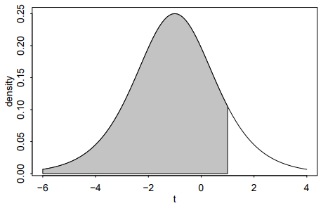
If we set $\beta_{0}=-\mu / \sigma$ and $\beta_{1}=1 / \sigma$, we now have a logistic regression model. We can illustrate this in the following example where we set $d=1$ and let $T$ have mean $-1$ and $\sigma=1$ :
$x<-\operatorname{seq}(-6,4,0.1)$
$y<-d \log _{\text {is }}(x$, location $=-1)$
plot (x,y, type=”1″, ylab=”density”, $x l a b=” t “)$
i1 $<-(x<1)$
polygon (c $(x[11], 1,-6), c(y[11], 0,0)$, col=’ gray’)
The plot in Figure $4.1$ shows a logistically distributed latent variable. We can see that this distribution is apparently very similar to the normal distribution. The shaded area represents the probability of getting an answer wrong. As the mean aptitude of this student is somewhat less than the difficulty of the question, this probability is substantially greater than one half.
This idea also arises in a bioassay where we might treat an animal, plant or person with some concentration of a treatment and observe the outcome. For example, suppose we are interested in the concentration of insecticide to be used in exterminating a pest. Insects will have varying tolerances for the toxin and will survive if their tolerance is greater than the dose. In this context, the term tolerance distribution for $T$ is used. Applications in several other areas exist where we observe only a binary outcome but believe this to be generated by some continuous but unobserved variable.
统计代写|广义线性模型代写generalized linear model代考|Link Functions
Until now we have used logit link function to connect the probability and the linear predictor. But other choices of link function are reasonable. We need a function that bounds the probability between zero and one. We also expect the link function to be monotone. It is conceivable that the success probability may go up and down as the linear predictor increases but this circumstance is best modeled by adding nonlinear components to the linear predictors such as quadratic terms rather than modifying the link function. The latent variable formulation suggests some other possibilities for the link function. Here are some choices which are implemented in the glm () function:
- Probit: $\eta=\Phi^{-1}(p)$ where $\Phi$ is the normal cumulative distribution function. This arises from a normally distributed latent variable.
- Complementary $\log -\log : \eta=\log (-\log (1-p))$. A Gumbel-distributed latent variable will lead to this.
- Cauchit: $\eta=\tan ^{-1}(\pi(p-1 / 2))$ which is motivated by a Cauchy-distributed latent variable.
We can illustrate the choices using some data from Bliss (1935) on the numbers of insects dying at different levels of insecticide concentration. We fit all four link functions:
These are not very different, but now look at a wider range from $[-4,8]$. We apply the predict function to each of the four models forming a matrix of predicted values. We label the columns and add the information about the dose. The tidyr package is useful for reformatting data from a wide format of multiple measured values per row to a long format where there is only one response value per row. This is accomplished using the gather () function. This format, where each row is an observation and each column is a variable, is the most convenient form for many $R$ analyses. Finally, the ggplot 2 package is useful for completing and well-labeled plot.
广义线性模型代考
统计代写|广义线性模型代写generalized linear model代考|Beta Regression
Beta 回归对于有界的响应很有用(0,1)比如比例。它也可以用于限制在其他有限区间内的变量,只需重新缩放到(0,1). 一个 Beta 分布的随机变量是有密度:
F(是∣一个,b)=Γ(一个+b)Γ(一个)Γ(b)是一个−1(1−是)b−1
对于参数一个,b和 Gamma 函数Γ(). 转换参数更方便,所以μ=一个/(一个+b)和φ=一个+b以便和是=μ和曾是是=μ(1−μ)/(1+ ∅). 然后我们可以链接线性预测器这使用这=G(μ)使用链接功能G用于二项式模型的任何选择都是合适的。
Beta 回归模型的实现可以在 Wood (2006) 的 macv 包中找到。我们可以将其应用于上一节中使用的哺乳动物睡眠。
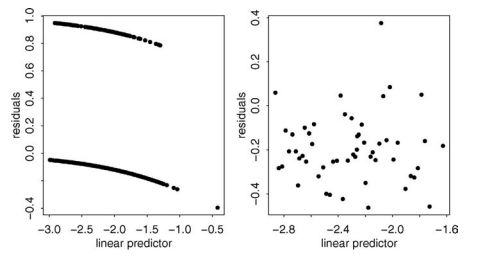
链接的默认选择是 logit 函数。的估计值φ是8.927. 该模型的拟合值与之前拟合的准二项式模型的比较显示没有实质性差异。基于 Beta 的模型的优点是完整的分布模型,它允许构建完整的预测分布,而不仅仅是点估计和标准误差。
统计代写|广义线性模型代写generalized linear model代考|Latent Variables
假设学生在测试中回答问题并且特定学生具有能力吨. 一个特定的问题可能有困难d并且学生只有在以下情况下才能得到正确的答案吨>d. 现在如果我们考虑d固定和吨作为具有密度的随机变量F和分布函数F,则学生答错的概率为:
p=磷(吨≤d)=F(d)
吨称为潜变量。假设分布吨是逻辑:
F(是)=经验(是−μ)/σ1+经验(是−μ)/σ
小号○
罗吉特(p)=−μ/σ+d/σ
如果我们设置b0=−μ/σ和b1=1/σ,我们现在有一个逻辑回归模型。我们可以在下面设置的示例中说明这一点d=1然后让吨有意思−1和σ=1 :
X<−序列(−6,4,0.1)
是<−d日志是 (X, 地点=−1)
绘图(x,y,类型=“1”,ylab=“密度”,Xl一个b=”吨“)
i1<−(X<1)
多边形(c(X[11],1,−6),C(是[11],0,0), col=’gray’)
图中的情节4.1显示了一个逻辑分布的潜变量。我们可以看到,这种分布显然与正态分布非常相似。阴影区域代表回答错误的概率。由于该学生的平均能力略低于问题的难度,因此该概率大大大于二分之一。
这个想法也出现在生物测定中,我们可能会对动物、植物或人进行一定程度的治疗并观察结果。例如,假设我们对用于消灭害虫的杀虫剂浓度感兴趣。昆虫对毒素有不同的耐受性,如果它们的耐受性大于剂量,它们就会存活下来。在这种情况下,术语公差分布吨用来。在其他几个领域的应用中,我们只观察到二元结果,但认为这是由一些连续但未观察到的变量产生的。
统计代写|广义线性模型代写generalized linear model代考|Link Functions
到目前为止,我们已经使用 logit 链接函数来连接概率和线性预测器。但链接功能的其他选择是合理的。我们需要一个将概率限制在零和一之间的函数。我们还期望链接函数是单调的。可以想象,随着线性预测器的增加,成功概率可能会上下波动,但这种情况最好通过向线性预测器添加非线性分量(例如二次项)而不是修改链接函数来建模。潜变量公式为链接函数提出了一些其他的可能性。以下是在 glm () 函数中实现的一些选项:
- 概率:这=披−1(p)在哪里披是正态累积分布函数。这是由一个正态分布的潜变量引起的。
- 补充日志−日志:这=日志(−日志(1−p)). 一个 Gumbel 分布的潜在变量将导致这一点。
- 考希特:这=棕褐色−1(圆周率(p−1/2))这是由柯西分布的潜在变量驱动的。
我们可以使用 Bliss (1935) 中关于在不同杀虫剂浓度水平下死亡的昆虫数量的一些数据来说明这些选择。我们适合所有四个链接功能:
这些并没有太大的不同,但现在从更广泛的范围来看[−4,8]. 我们将预测函数应用于形成预测值矩阵的四个模型中的每一个。我们标记列并添加有关剂量的信息。tidyr 包可用于将数据从每行多个测量值的宽格式重新格式化为每行只有一个响应值的长格式。这是使用gather () 函数完成的。这种格式,其中每一行是一个观察值,每一列是一个变量,对于许多人来说是最方便的形式R分析。最后,ggplot 2 包对于完成和标记良好的绘图很有用。

统计代写请认准statistics-lab™. statistics-lab™为您的留学生涯保驾护航。
金融工程代写
金融工程是使用数学技术来解决金融问题。金融工程使用计算机科学、统计学、经济学和应用数学领域的工具和知识来解决当前的金融问题,以及设计新的和创新的金融产品。
非参数统计代写
非参数统计指的是一种统计方法,其中不假设数据来自于由少数参数决定的规定模型;这种模型的例子包括正态分布模型和线性回归模型。
广义线性模型代考
广义线性模型(GLM)归属统计学领域,是一种应用灵活的线性回归模型。该模型允许因变量的偏差分布有除了正态分布之外的其它分布。
术语 广义线性模型(GLM)通常是指给定连续和/或分类预测因素的连续响应变量的常规线性回归模型。它包括多元线性回归,以及方差分析和方差分析(仅含固定效应)。
有限元方法代写
有限元方法(FEM)是一种流行的方法,用于数值解决工程和数学建模中出现的微分方程。典型的问题领域包括结构分析、传热、流体流动、质量运输和电磁势等传统领域。
有限元是一种通用的数值方法,用于解决两个或三个空间变量的偏微分方程(即一些边界值问题)。为了解决一个问题,有限元将一个大系统细分为更小、更简单的部分,称为有限元。这是通过在空间维度上的特定空间离散化来实现的,它是通过构建对象的网格来实现的:用于求解的数值域,它有有限数量的点。边界值问题的有限元方法表述最终导致一个代数方程组。该方法在域上对未知函数进行逼近。[1] 然后将模拟这些有限元的简单方程组合成一个更大的方程系统,以模拟整个问题。然后,有限元通过变化微积分使相关的误差函数最小化来逼近一个解决方案。
tatistics-lab作为专业的留学生服务机构,多年来已为美国、英国、加拿大、澳洲等留学热门地的学生提供专业的学术服务,包括但不限于Essay代写,Assignment代写,Dissertation代写,Report代写,小组作业代写,Proposal代写,Paper代写,Presentation代写,计算机作业代写,论文修改和润色,网课代做,exam代考等等。写作范围涵盖高中,本科,研究生等海外留学全阶段,辐射金融,经济学,会计学,审计学,管理学等全球99%专业科目。写作团队既有专业英语母语作者,也有海外名校硕博留学生,每位写作老师都拥有过硬的语言能力,专业的学科背景和学术写作经验。我们承诺100%原创,100%专业,100%准时,100%满意。
随机分析代写
随机微积分是数学的一个分支,对随机过程进行操作。它允许为随机过程的积分定义一个关于随机过程的一致的积分理论。这个领域是由日本数学家伊藤清在第二次世界大战期间创建并开始的。
时间序列分析代写
随机过程,是依赖于参数的一组随机变量的全体,参数通常是时间。 随机变量是随机现象的数量表现,其时间序列是一组按照时间发生先后顺序进行排列的数据点序列。通常一组时间序列的时间间隔为一恒定值(如1秒,5分钟,12小时,7天,1年),因此时间序列可以作为离散时间数据进行分析处理。研究时间序列数据的意义在于现实中,往往需要研究某个事物其随时间发展变化的规律。这就需要通过研究该事物过去发展的历史记录,以得到其自身发展的规律。
回归分析代写
多元回归分析渐进(Multiple Regression Analysis Asymptotics)属于计量经济学领域,主要是一种数学上的统计分析方法,可以分析复杂情况下各影响因素的数学关系,在自然科学、社会和经济学等多个领域内应用广泛。
MATLAB代写
MATLAB 是一种用于技术计算的高性能语言。它将计算、可视化和编程集成在一个易于使用的环境中,其中问题和解决方案以熟悉的数学符号表示。典型用途包括:数学和计算算法开发建模、仿真和原型制作数据分析、探索和可视化科学和工程图形应用程序开发,包括图形用户界面构建MATLAB 是一个交互式系统,其基本数据元素是一个不需要维度的数组。这使您可以解决许多技术计算问题,尤其是那些具有矩阵和向量公式的问题,而只需用 C 或 Fortran 等标量非交互式语言编写程序所需的时间的一小部分。MATLAB 名称代表矩阵实验室。MATLAB 最初的编写目的是提供对由 LINPACK 和 EISPACK 项目开发的矩阵软件的轻松访问,这两个项目共同代表了矩阵计算软件的最新技术。MATLAB 经过多年的发展,得到了许多用户的投入。在大学环境中,它是数学、工程和科学入门和高级课程的标准教学工具。在工业领域,MATLAB 是高效研究、开发和分析的首选工具。MATLAB 具有一系列称为工具箱的特定于应用程序的解决方案。对于大多数 MATLAB 用户来说非常重要,工具箱允许您学习和应用专业技术。工具箱是 MATLAB 函数(M 文件)的综合集合,可扩展 MATLAB 环境以解决特定类别的问题。可用工具箱的领域包括信号处理、控制系统、神经网络、模糊逻辑、小波、仿真等。