如果你也在 怎样代写数值分析和优化numerical analysis and optimazation这个学科遇到相关的难题,请随时右上角联系我们的24/7代写客服。
数值分析是根据数学模型提出的问题,建立求解问题的数值计算方法并进行方法的理论分析,直到编制出算法程序上机计算得到数值结果,以及对结果进行分析。
statistics-lab™ 为您的留学生涯保驾护航 在代写数值分析和优化numerical analysis and optimazation方面已经树立了自己的口碑, 保证靠谱, 高质且原创的统计Statistics代写服务。我们的专家在代写数值分析和优化numerical analysis and optimazation方面经验极为丰富,各种代写数值分析和优化numerical analysis and optimazation相关的作业也就用不着说。
我们提供的数值分析和优化numerical analysis and optimazation及其相关学科的代写,服务范围广, 其中包括但不限于:
- Statistical Inference 统计推断
- Statistical Computing 统计计算
- Advanced Probability Theory 高等楖率论
- Advanced Mathematical Statistics 高等数理统计学
- (Generalized) Linear Models 广义线性模型
- Statistical Machine Learning 统计机器学习
- Longitudinal Data Analysis 纵向数据分析
- Foundations of Data Science 数据科学基础
统计代写|数值分析和优化代写numerical analysis and optimazation代考|Householder Reflections
Definition $2.5$ (Householder reflections). Let $\mathbf{u} \in \mathbb{R}^{n}$ be a non-zero vector. The $n \times n$ matrix of the form
$$
I-2 \frac{\mathbf{u}^{T}}{| \mathbf{u}^{2}}
$$
is called a Householder reflection.
A Householder reflection describes a reflection about a hyperplane which is orthogonal to the vector $\mathbf{u} /|\mathbf{u}|$ and which contains the origin. Each such matrix is symmetric and orthogonal, since
$$
\begin{aligned}
\left(I-2 \frac{\mathbf{u} \mathbf{u}^{T}}{|\mathbf{u}|^{2}}\right)^{T}\left(I-2 \frac{\mathbf{u u}^{T}}{|\mathbf{u}|^{2}}\right) &=\left(I-2 \frac{\mathbf{u} \mathbf{u}^{T}}{|\mathbf{u}|^{2}}\right)^{2} \
&=I-4 \frac{\mathbf{u} \mathbf{u}^{T}}{|\mathbf{u}|^{2}}+4 \frac{\mathbf{u}\left(\mathbf{u}^{T} \mathbf{u}\right) \mathbf{u}^{T}}{|\mathbf{u}|^{4}}=I .
\end{aligned}
$$
We can use Householder reflections instead of Givens rotations to calculate a QR factorization.
With each multiplication of an $n \times m$ matrix $A$ by a Householder reflection we want to introduce zeros under the diagonal in an entire column. To start with we construct a reflection which transforms the first nonzero column $\mathbf{a} \in$ $\mathbf{R}^{n}$ of $A$ into a multiple of the first unit vector $\mathbf{e}{1}$. In other words we want to choose $\mathbf{u} \in \mathbb{R}^{n}$ such that the last $n-1$ entries of $$ \left(I-2 \frac{\mathbf{u}^{T}}{|\mathbf{u}|^{2}}\right) \mathbf{a}=\mathbf{a}-2 \frac{\mathbf{u}^{T} \mathbf{a}}{|\mathbf{u}|^{2}} \mathbf{u} $$ vanish. Since we are free to choose the length of u, we normalize it such that $|u|^{2}=2 \mathbf{u}^{T} \mathbf{a}$, which is possible since $\mathbf{a} \neq 0$. The right side of Equation (2.3) then simplifies to $\mathbf{a}-\mathbf{u}$ and we have $u{i}=a_{i}$ for $i=2, \ldots, n$. Using this we can rewrite the normalization as
$$
2 u_{1} a_{1}+2 \sum_{i=2}^{n} a_{i}^{2}=u_{1}^{2}+\sum_{i=2}^{n} a_{i}^{2}
$$
Gathering the terms and extending the sum, we have
$$
u_{1}^{2}-2 u_{1} a_{1}+a_{1}^{2}-\sum_{i=1}^{n} a_{i}^{2}=0 \Leftrightarrow\left(u_{1}-a_{1}\right)^{2}=\sum_{i=1}^{n} a_{i}^{2} .
$$
Thus $u_{1}=a_{1} \pm|\mathbf{a}|$. In numerical applications it is usual to let the sign be the same sign as $a_{1}$ to avoid $|\mathbf{u}|$ becoming too small, since a division by a very small number can lead to numerical difficulties.
统计代写|数值分析和优化代写numerical analysis and optimazation代考|Linear Least Squares
Consider a system of linear equations $A \mathbf{x}=\mathbf{b}$ where $A$ is an $n \times m$ matrix and $\mathbf{b} \in \mathbb{R}^{n}$.
In the case $n<m$ there are not enough equations to define a unique solution. The system is called under-determined. All possible solutions form a vector space of dimension $r$, where $r \leq m-n$. This problem seldom arises in practice, since generally we choose a solution space in accordance with the available data. An example, however, are cubic splines, which we will encounter later.
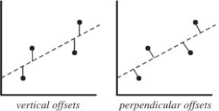
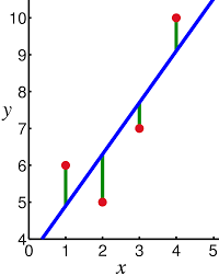
In the case $n>m$ there are more equations than unknowns. The system is called over-determined. This situation may arise where a simple data model is fitted to a large number of data points. Problems of this form occur frequently when we collect $n$ observations which often carry measurement errors, and we want to build an $m$-dimensional linear model where generally $m$ is much smaller than $n$. In statistics this is known as linear regression. Many machine learning algorithms have been developed to address this problem (see for example [2] C. M. Bishop Pattern Recognition and Machine Learning).
We consider the simplest approach, that is, we seek $\mathbf{x} \in \mathbb{R}^{m}$ that minimizes the Euclidean norm $|A \mathbf{x}-\mathbf{b}|$. This is known as the least-squares problem.
统计代写|数值分析和优化代写numerical analysis and optimazation代考|Iterative Schemes and Splitting
Given a linear system of the form $A \mathbf{x}=\mathbf{b}$, where $A$ is an $n \times n$ matrix and $\mathbf{x}, \mathbf{b} \in \mathbb{R}^{n}$, solving it by factorization is frequently very expensive for large $n$. However, we can rewrite it in the form
$$
(A-B) \mathbf{x}=-B \mathbf{x}+\mathbf{b}
$$
where the matrix $B$ is chosen in such a way that $A-B$ is non-singular and the system $(A-B) \mathbf{x}=\mathbf{y}$ is easily solved for any right-hand side $\mathbf{y}$. A simple iterative scheme starts with an estimate $\mathbf{x}^{(0)} \in \mathbb{R}^{n}$ of the solution (this could be arbitrary) and generates the sequence $\mathbf{x}^{(k)}, k=1,2, \ldots$, by solving
$$
(A-B) \mathbf{x}^{(k+1)}=-B \mathbf{x}^{(k)}+\mathbf{b} .
$$
This technique is called splitting. If the sequence converges to a limit, $\lim _{k \rightarrow \infty} \mathbf{x}^{(k)}=\hat{\mathbf{x}}$, then taking the limit on both sides of Equation (2.4) gives $(A-B) \hat{\mathbf{x}}=-B \hat{\mathbf{x}}+\mathbf{b}$. Hence $\hat{\mathbf{x}}$ is a solution of $A \mathbf{x}=\mathbf{b}$.
What are the necessary and sufficient conditions for convergence? Suppose that $A$ is non-singular and therefore has a unique solution $\mathbf{x}^{}$. Since $\mathbf{x}^{}$ solves $A \mathbf{x}=\mathbf{b}$, it also satisfies $(A-B) \mathbf{x}^{}=-B \mathbf{x}^{}+\mathbf{b}$. Subtracting this equation from (2.4) gives
$$
(A-B)\left(\mathbf{x}^{(k+1)}-\mathbf{x}^{}\right)=-B\left(\mathbf{x}^{(k)}-\mathbf{x}^{}\right)
$$
We denote $\mathbf{x}^{(k)}-\mathbf{x}^{*}$ by $\mathbf{e}^{(k)}$. It is the error in the $k^{\text {th }}$ iteration. Since $A-B$ is non-singular, we can write
$$
\mathbf{e}^{(k+1)}=-(A-B)^{-1} B \mathbf{e}^{(k)}
$$
The matrix $H:=-(A-B)^{-1} B$ is known as the iteration matrix. In practical applications $H$ is not calculated. We analyze its properties theoretically in order to determine whether or not we have convergence. We will encounter such analyses later on.
数值分析代写
统计代写|数值分析和优化代写numerical analysis and optimazation代考|Householder Reflections
定义2.5(住户反思)。让在∈Rn是一个非零向量。这n×n形式的矩阵
一世−2在吨|在2
称为 Householder 反射。
Householder反射描述了关于与向量正交的超平面的反射在/|在|其中包含起源。每个这样的矩阵都是对称且正交的,因为
(一世−2在在吨|在|2)吨(一世−2在在吨|在|2)=(一世−2在在吨|在|2)2 =一世−4在在吨|在|2+4在(在吨在)在吨|在|4=一世.
我们可以使用 Householder 反射而不是 Givens 旋转来计算 QR 分解。
每次乘以一个n×米矩阵一种通过 Householder 反射,我们希望在整个列的对角线下方引入零。首先,我们构造一个反射来转换第一个非零列一种∈ Rn的一种成第一个单位向量的倍数和1. 换句话说,我们要选择在∈Rn这样最后n−1的条目(一世−2在吨|在|2)一种=一种−2在吨一种|在|2在消失。由于我们可以自由选择 u 的长度,因此我们对其进行归一化,使得|在|2=2在吨一种,这是可能的,因为一种≠0. 等式 (2.3) 的右侧则简化为一种−在我们有在一世=一种一世为了一世=2,…,n. 使用它,我们可以将规范化重写为
2在1一种1+2∑一世=2n一种一世2=在12+∑一世=2n一种一世2
收集条款并扩展总和,我们有
在12−2在1一种1+一种12−∑一世=1n一种一世2=0⇔(在1−一种1)2=∑一世=1n一种一世2.
因此在1=一种1±|一种|. 在数值应用中,通常让符号与一种1避免|在|变得太小,因为除以非常小的数字会导致数字困难。
统计代写|数值分析和优化代写numerical analysis and optimazation代考|Linear Least Squares
考虑一个线性方程组一种X=b在哪里一种是一个n×米矩阵和b∈Rn.
在这种情况下n<米没有足够的方程来定义唯一解。该系统称为欠定系统。所有可能的解形成一个维向量空间r, 在哪里r≤米−n. 这个问题在实践中很少出现,因为通常我们根据可用数据选择解空间。然而,一个例子是三次样条,我们稍后会遇到。
在这种情况下n>米方程多于未知数。该系统称为超定。当一个简单的数据模型适合大量数据点时,可能会出现这种情况。这种形式的问题在我们收集时经常出现n经常带有测量误差的观察结果,我们想建立一个米维线性模型,其中通常米远小于n. 在统计学中,这被称为线性回归。已经开发了许多机器学习算法来解决这个问题(参见例如 [2] CM Bishop Pattern Recognition and Machine Learning)。
我们考虑最简单的方法,即我们寻求X∈R米最小化欧几里得范数|一种X−b|. 这被称为最小二乘问题。
统计代写|数值分析和优化代写numerical analysis and optimazation代考|Iterative Schemes and Splitting
给定一个线性系统的形式一种X=b, 在哪里一种是一个n×n矩阵和X,b∈Rn, 通过因式分解解决它通常对于大型n. 但是,我们可以将其重写为形式
(一种−乙)X=−乙X+b
矩阵在哪里乙以这样的方式选择一种−乙是非奇异的并且系统(一种−乙)X=是很容易解决任何右手边是. 一个简单的迭代方案从估计开始X(0)∈Rn解(这可以是任意的)并生成序列X(ķ),ķ=1,2,…, 通过求解
(一种−乙)X(ķ+1)=−乙X(ķ)+b.
这种技术称为分裂。如果序列收敛到一个极限,林ķ→∞X(ķ)=X^,然后在等式(2.4)两边取极限,得到(一种−乙)X^=−乙X^+b. 因此X^是一个解决方案一种X=b.
收敛的充分必要条件是什么?假设一种是非奇异的,因此具有唯一的解决方案X. 自从X解决一种X=b, 也满足(一种−乙)X=−乙X+b. 从 (2.4) 中减去这个方程得到
(一种−乙)(X(ķ+1)−X)=−乙(X(ķ)−X)
我们表示X(ķ)−X∗经过和(ķ). 这是中的错误ķth 迭代。自从一种−乙是非奇异的,我们可以写
和(ķ+1)=−(一种−乙)−1乙和(ķ)
矩阵H:=−(一种−乙)−1乙称为迭代矩阵。在实际应用中H不计算。我们从理论上分析它的性质,以确定我们是否具有收敛性。我们稍后会遇到这样的分析。

统计代写请认准statistics-lab™. statistics-lab™为您的留学生涯保驾护航。统计代写|python代写代考
随机过程代考
在概率论概念中,随机过程是随机变量的集合。 若一随机系统的样本点是随机函数,则称此函数为样本函数,这一随机系统全部样本函数的集合是一个随机过程。 实际应用中,样本函数的一般定义在时间域或者空间域。 随机过程的实例如股票和汇率的波动、语音信号、视频信号、体温的变化,随机运动如布朗运动、随机徘徊等等。
贝叶斯方法代考
贝叶斯统计概念及数据分析表示使用概率陈述回答有关未知参数的研究问题以及统计范式。后验分布包括关于参数的先验分布,和基于观测数据提供关于参数的信息似然模型。根据选择的先验分布和似然模型,后验分布可以解析或近似,例如,马尔科夫链蒙特卡罗 (MCMC) 方法之一。贝叶斯统计概念及数据分析使用后验分布来形成模型参数的各种摘要,包括点估计,如后验平均值、中位数、百分位数和称为可信区间的区间估计。此外,所有关于模型参数的统计检验都可以表示为基于估计后验分布的概率报表。
广义线性模型代考
广义线性模型(GLM)归属统计学领域,是一种应用灵活的线性回归模型。该模型允许因变量的偏差分布有除了正态分布之外的其它分布。
statistics-lab作为专业的留学生服务机构,多年来已为美国、英国、加拿大、澳洲等留学热门地的学生提供专业的学术服务,包括但不限于Essay代写,Assignment代写,Dissertation代写,Report代写,小组作业代写,Proposal代写,Paper代写,Presentation代写,计算机作业代写,论文修改和润色,网课代做,exam代考等等。写作范围涵盖高中,本科,研究生等海外留学全阶段,辐射金融,经济学,会计学,审计学,管理学等全球99%专业科目。写作团队既有专业英语母语作者,也有海外名校硕博留学生,每位写作老师都拥有过硬的语言能力,专业的学科背景和学术写作经验。我们承诺100%原创,100%专业,100%准时,100%满意。
机器学习代写
随着AI的大潮到来,Machine Learning逐渐成为一个新的学习热点。同时与传统CS相比,Machine Learning在其他领域也有着广泛的应用,因此这门学科成为不仅折磨CS专业同学的“小恶魔”,也是折磨生物、化学、统计等其他学科留学生的“大魔王”。学习Machine learning的一大绊脚石在于使用语言众多,跨学科范围广,所以学习起来尤其困难。但是不管你在学习Machine Learning时遇到任何难题,StudyGate专业导师团队都能为你轻松解决。
多元统计分析代考
基础数据: $N$ 个样本, $P$ 个变量数的单样本,组成的横列的数据表
变量定性: 分类和顺序;变量定量:数值
数学公式的角度分为: 因变量与自变量
时间序列分析代写
随机过程,是依赖于参数的一组随机变量的全体,参数通常是时间。 随机变量是随机现象的数量表现,其时间序列是一组按照时间发生先后顺序进行排列的数据点序列。通常一组时间序列的时间间隔为一恒定值(如1秒,5分钟,12小时,7天,1年),因此时间序列可以作为离散时间数据进行分析处理。研究时间序列数据的意义在于现实中,往往需要研究某个事物其随时间发展变化的规律。这就需要通过研究该事物过去发展的历史记录,以得到其自身发展的规律。
回归分析代写
多元回归分析渐进(Multiple Regression Analysis Asymptotics)属于计量经济学领域,主要是一种数学上的统计分析方法,可以分析复杂情况下各影响因素的数学关系,在自然科学、社会和经济学等多个领域内应用广泛。
MATLAB代写
MATLAB 是一种用于技术计算的高性能语言。它将计算、可视化和编程集成在一个易于使用的环境中,其中问题和解决方案以熟悉的数学符号表示。典型用途包括:数学和计算算法开发建模、仿真和原型制作数据分析、探索和可视化科学和工程图形应用程序开发,包括图形用户界面构建MATLAB 是一个交互式系统,其基本数据元素是一个不需要维度的数组。这使您可以解决许多技术计算问题,尤其是那些具有矩阵和向量公式的问题,而只需用 C 或 Fortran 等标量非交互式语言编写程序所需的时间的一小部分。MATLAB 名称代表矩阵实验室。MATLAB 最初的编写目的是提供对由 LINPACK 和 EISPACK 项目开发的矩阵软件的轻松访问,这两个项目共同代表了矩阵计算软件的最新技术。MATLAB 经过多年的发展,得到了许多用户的投入。在大学环境中,它是数学、工程和科学入门和高级课程的标准教学工具。在工业领域,MATLAB 是高效研究、开发和分析的首选工具。MATLAB 具有一系列称为工具箱的特定于应用程序的解决方案。对于大多数 MATLAB 用户来说非常重要,工具箱允许您学习和应用专业技术。工具箱是 MATLAB 函数(M 文件)的综合集合,可扩展 MATLAB 环境以解决特定类别的问题。可用工具箱的领域包括信号处理、控制系统、神经网络、模糊逻辑、小波、仿真等。