如果你也在 怎样代写时间序列分析Time-Series Analysis这个学科遇到相关的难题,请随时右上角联系我们的24/7代写客服。
时间序列分析是分析在一个时间间隔内收集的一系列数据点的具体方式。在时间序列分析中,分析人员在设定的时间段内以一致的时间间隔记录数据点,而不仅仅是间歇性或随机地记录数据点。
statistics-lab™ 为您的留学生涯保驾护航 在代写时间序列分析Time-Series Analysis方面已经树立了自己的口碑, 保证靠谱, 高质且原创的统计Statistics代写服务。我们的专家在代写时间序列分析Time-Series Analysis代写方面经验极为丰富,各种代写时间序列分析Time-Series Analysis相关的作业也就用不着说。
我们提供的时间序列分析Time-Series Analysis及其相关学科的代写,服务范围广, 其中包括但不限于:
- Statistical Inference 统计推断
- Statistical Computing 统计计算
- Advanced Probability Theory 高等概率论
- Advanced Mathematical Statistics 高等数理统计学
- (Generalized) Linear Models 广义线性模型
- Statistical Machine Learning 统计机器学习
- Longitudinal Data Analysis 纵向数据分析
- Foundations of Data Science 数据科学基础
统计代写|时间序列分析代写Time-Series Analysis代考|Frequency Resolution of Autoregressive Spectral Analysis
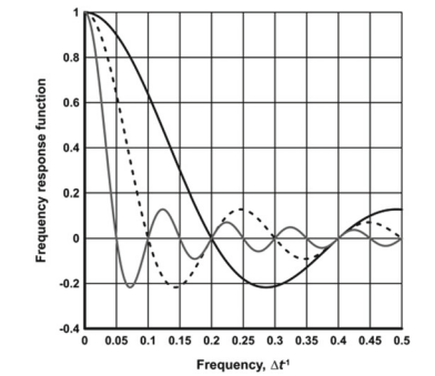
The AR (or MEM) spectral estimation provides an analytical formula for the estimated spectrum. It means that the spectral resolution in the formula is such that the value of spectral density can be calculated at any frequency. This is true, but the actual resolution is defined by the AR order: the number of extrema and inflection points in the spectral curve corresponding to an $\operatorname{AR}(p)$ model cannot be higher than $p$ (see Sect. 4.3). Therefore, a high resolution requires a high AR order, but a high-order model cannot be obtained with a short time series.
By definition, a linearly regular random process does not contain any strictly periodic components. This feature may cause some doubts about the ability of parametric time series analysis designed for regular processes to detect sharp peaks at frequencies which are close to each other, for example, when the data contain harmonic oscillations. Actually, the ability of autoregressive spectral analysis in this respect is very high under just one condition: getting accurate results requires having enough data for analysis. (Certainly, this requirement holds for all nonparametric method of spectral analysis such as Blackman and Tukey’s, MTM, Welch’s, etc.)
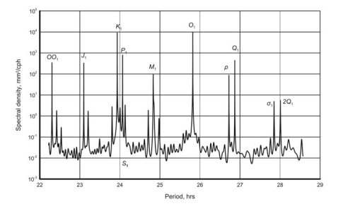
A unique case of harmonic oscillations with perfectly known frequencies within the Earth system is tides. The frequencies of tidal constituents are known precisely from astronomy; the amplitudes are determined from observations. The autoregressive analysis in the frequency domain provides a convenient tool for estimating frequencies of harmonic oscillations that are contained in time series of tidal phenomena. If the frequencies are determined correctly in sea level observations, one may hope that they will also be determined correctly in any other stationary data.
The example below is designed to verify how accurately the maximum entropy spectral analysis can determine the frequencies of tidal constituents by analyzing the time series of sea level at station 9414317 , Pier $221 / 2$, San Francisco, USA, using $10^{5}$ hourly sea level observations starting from January 28,2000 . The data source is $# 3$ in Appendix. A part of the record (about 50 days) is shown in Fig. 4.7. The tides obviously dominate the record.
统计代写|时间序列分析代写Time-Series Analysis代考|Example of AR Analysis in Time and Frequency Domains
Consider the entire process of time series analysis using as an example the annual values of Tripole Index (TPI) for the Interdecadal Pacific Oscillation (Henley et al. 2015). The time series shown in Fig. $4.9$ extends from 1854 through $2018(N=165)$; it is closely related to other El Niño-Southern Oscillation indices but differs from them in some respects. The data source is taken from the Web site #5 in Appendix to this chapter. The time series does not contain any statistically significant trend, and its behavior allows one to assume, without any further analysis, that it can be treated as a sample of a stationary random process. The test for Gaussianity showed that the probability density function of this time series can be regarded as normal.
The time series has been analyzed in the time domain by fitting to it $\mathrm{AR}(p)$ models of orders from $p=0$ through $p=16$ (one-tenth of the time series length). Three of the five order selection criteria used in this book have chosen the order $p=3$ :
$$
x_{t} \approx 0.46 x_{t-1}-0.29 x_{t-2}+0.15 x_{t-3}+a_{t}
$$
The RMS error of all estimated AR coefficients equals to approximately $0.08$ so that the coefficients are statistically significant at the confidence level $0.9$ used in this book.
The estimates of the mean value and standard deviation are $\bar{x} \approx-0.15$ and $\hat{\sigma}_{x} \approx 0.61$. The respective confidence intervals for the mean value and variance estimates obtained for the TPI time series expressed with model (4.11) are [ $-0.25$,
$-0.04]$ and $[0.55,0.68]$. These confidence intervals are determined in accordance with Eqs. (4.1) -(4.4) using estimates of the numbers of independent observations $\bar{N}=93$ and $\hat{N}=130$ obtained for the AR(3) model (4.11). These values are calculated through the correlation function estimate under the assumption that the correlation function $r(k)$ at lags $k=1,2,3$ coincides with the sample estimates while its further values behave in the maximum entropy mode. This correlation function obtained according to Eq. (4.5) diminishes very fast so that the numbers of independent observations $\bar{N}$ and $\hat{N}$ do not differ drastically from the total number of observations $N$.
The innovation sequence variance $\sigma_{a}^{2} \approx 0.31$ and the predictability (persistence) criterion $r_{e}(1)=\sqrt{1-\sigma_{a}^{2} / \sigma_{x}^{2}}$ equals $0.17$ meaning that the unpredictable innovation sequence $a_{t}$ plays a dominant role in the time series of Tripole Index. This time series is quite close to a white noise sequence, and the variance of its prediction errors will be high.
统计代写|时间序列分析代写Time-Series Analysis代考|Properties of Climate Indices
At climatic time scales, the basic statistical properties of a large number of geophysical time series-about 3000 -has been summarized in the fundamental work by Dobrovolski $(2000)$ dealing with stochastic models of scalar climatic data. The time series in that book include surface temperature, atmospheric pressure, precipitation, sea level, and some other geophysical variables observed at individual stations; the data set includes 195 time series of sea surface temperature averaged within $5^{\circ} \times 5^{\circ}$ squares. Most of those time series are best approximated with either a white noise or a Markov process (Dobrovolski 2000 , p. 135). The white noise model AR(0) can be justly regarded as a specific case of the $\mathrm{AR}(1)$ model. The prevalence of the $\mathrm{AR}(1)$ model for climatic time series obtained without large-scale spatial averaging has been noted recently in Privalsky and Yushkov (2018), but the results given in Dobrovolski $(2000)$ are based upon a much larger observation base.
In this section, we will complement the available information by studying first a number of geophysical time series that are often used as climate indicators or indices; their names usually contain the term “oscillation” or “index.” The list is given in Table 5.1, and the data sources are shown in the Appendix to this chapter. In all cases, the value of $\Delta t$ is one year. Along with the optimal AR orders $p$ for the time series, the table contains the values of statistical predictability criterion (3.7): $r_{e}(1)=\sqrt{1-\sigma_{a}^{2} / \sigma_{x}^{2}}$, where $\sigma_{x}^{2}$ and $\sigma_{a}^{2}$ are the time series variance and the variance of its innovation sequence.
The sources of data listed in the table are given in Appendix to this chapter: the numbers in the first column of the table coincide with the numbers in the Appendix.
Two characteristic features are common for the time series in Table 5.1: all of them can be regarded as Gaussian, and, with one exception, all of them have low statistical predictability. This means that they present sample records of random processes similar to a white noise; that is, their behavior in the time domain is very irregular, and, consequently, none of them contains oscillations as the term is understood in physics. The exception is the relatively high predictability of the Atlantic Multidecadal Oscillation. Thus, judging by the low optimal AR orders and the low predictability, one may say that though the optimal model for most of these time series is not AR(1) their behavior does not contradict the assumption of the Markov character of climate variability and that the value of the autoregressive coefficient is significantly smaller than one.
时间序列分析代考
统计代写|时间序列分析代写Time-Series Analysis代考|Frequency Resolution of Autoregressive Spectral Analysis
AR(或 MEM)谱估计为估计的谱提供了一个分析公式。这意味着公式中的光谱分辨率使得光谱密度的值可以在任何频率下计算。这是真的,但实际分辨率由 AR 阶定义:光谱曲线中极值和拐点的数量对应于和(p)型号不能高于p(见第 4.3 节)。因此,高分辨率需要高AR阶数,而时间序列短却无法得到高阶模型。
根据定义,线性规则随机过程不包含任何严格的周期性分量。此功能可能会导致对为常规过程设计的参数时间序列分析检测彼此接近的频率处的尖峰的能力产生一些疑问,例如,当数据包含谐波振荡时。实际上,自回归光谱分析在这方面的能力非常高,仅在一个条件下:获得准确的结果需要有足够的数据进行分析。(当然,此要求适用于所有非参数光谱分析方法,例如 Blackman 和 Tukey’s、MTM、Welch’s 等)
地球系统内具有完全已知频率的谐波振荡的一个独特情况是潮汐。潮汐成分的频率可以从天文学中准确得知;幅度由观察确定。频域中的自回归分析为估计包含在潮汐现象时间序列中的谐波振荡频率提供了一种方便的工具。如果在海平面观测中正确确定了频率,人们可能希望在任何其他固定数据中也能正确确定频率。
下面的示例旨在通过分析码头 9414317 站的海平面时间序列来验证最大熵谱分析如何准确地确定潮汐成分的频率221/2,美国旧金山,使用105从 2000 年 1 月 28 日开始的每小时海平面观测。数据源是# 3# 3在附录中。部分记录(约 50 天)如图 4.7 所示。潮汐显然占主导地位。
统计代写|时间序列分析代写Time-Series Analysis代考|Example of AR Analysis in Time and Frequency Domains
以年代际太平洋涛动的三极子指数 (TPI) 的年度值为例,考虑时间序列分析的整个过程(Henley 等人,2015 年)。时间序列如图所示。4.9从 1854 年延伸到2018(ñ=165); 它与其他厄尔尼诺-南方涛动指数密切相关,但在某些方面有所不同。数据源取自本章附录中的网站#5。时间序列不包含任何统计上显着的趋势,并且它的行为允许人们在没有任何进一步分析的情况下假设它可以被视为平稳随机过程的样本。高斯性检验表明,该时间序列的概率密度函数可视为正态。
时间序列已通过拟合在时域中进行了分析一个R(p)订单型号来自p=0通过p=16(时间序列长度的十分之一)。本书中使用的五个订单选择标准中的三个选择了订单p=3 :
X吨≈0.46X吨−1−0.29X吨−2+0.15X吨−3+一个吨
所有估计的 AR 系数的 RMS 误差大约等于0.08使得系数在置信水平上具有统计显着性0.9本书中使用。
平均值和标准差的估计是X¯≈−0.15和σ^X≈0.61. 用模型 (4.11) 表示的 TPI 时间序列的平均值和方差估计值各自的置信区间为 [−0.25,
−0.04]和[0.55,0.68]. 这些置信区间是根据方程式确定的。(4.1) -(4.4) 使用独立观察次数的估计ñ¯=93和ñ^=130为 AR(3) 模型 (4.11) 获得。这些值是在相关函数的假设下通过相关函数估计计算得出的r(ķ)在滞后ķ=1,2,3与样本估计值一致,而其进一步的值表现为最大熵模式。该相关函数根据方程式获得。(4.5) 减少得非常快,因此独立观察的数量ñ¯和ñ^与观察总数没有太大差异ñ.
创新序列方差σ一个2≈0.31和可预测性(持久性)标准r和(1)=1−σ一个2/σX2等于0.17意味着不可预测的创新序列一个吨在三极子指数的时间序列中起主导作用。这个时间序列非常接近白噪声序列,其预测误差的方差会很大。
统计代写|时间序列分析代写Time-Series Analysis代考|Properties of Climate Indices
在气候时间尺度上,Dobrovolski 在基础工作中总结了大量地球物理时间序列(约 3000 个)的基本统计特性(2000)处理标量气候数据的随机模型。那本书中的时间序列包括地表温度、大气压力、降水、海平面和在各个站观测到的其他一些地球物理变量;该数据集包括 195 个时间序列的平均海表温度5∘×5∘正方形。大多数这些时间序列最好用白噪声或马尔可夫过程来近似(Dobrovolski 2000,第 135 页)。白噪声模型 AR(0) 可以公正地看作是一个R(1)模型。的流行一个R(1)最近在 Privalsky 和 Yushkov (2018) 中注意到了在没有大尺度空间平均的情况下获得的气候时间序列模型,但在 Dobrovolski 中给出的结果(2000)是基于更大的观察基础。
在本节中,我们将通过首先研究一些经常用作气候指标或指数的地球物理时间序列来补充现有信息;它们的名称通常包含术语“振荡”或“指数”。列表见表 5.1,数据来源见本章附录。在所有情况下,价值Δ吨是一年。连同最佳的 AR 订单p对于时间序列,该表包含统计可预测性标准 (3.7) 的值:r和(1)=1−σ一个2/σX2, 在哪里σX2和σ一个2是时间序列方差及其创新序列的方差。
表中数据来源见本章附录:表中第一栏数字与附录数字一致。
表 5.1 中的时间序列有两个共同的特征:它们都可以被认为是高斯的,并且除了一个例外,它们都具有低的统计可预测性。这意味着它们呈现类似于白噪声的随机过程的样本记录;也就是说,它们在时域中的行为非常不规则,因此它们都不包含物理学中所理解的振荡。例外是大西洋多年代际涛动的相对较高的可预测性。因此,从低最优 AR 阶数和低可预测性来看,

统计代写请认准statistics-lab™. statistics-lab™为您的留学生涯保驾护航。
金融工程代写
金融工程是使用数学技术来解决金融问题。金融工程使用计算机科学、统计学、经济学和应用数学领域的工具和知识来解决当前的金融问题,以及设计新的和创新的金融产品。
非参数统计代写
非参数统计指的是一种统计方法,其中不假设数据来自于由少数参数决定的规定模型;这种模型的例子包括正态分布模型和线性回归模型。
广义线性模型代考
广义线性模型(GLM)归属统计学领域,是一种应用灵活的线性回归模型。该模型允许因变量的偏差分布有除了正态分布之外的其它分布。
术语 广义线性模型(GLM)通常是指给定连续和/或分类预测因素的连续响应变量的常规线性回归模型。它包括多元线性回归,以及方差分析和方差分析(仅含固定效应)。
有限元方法代写
有限元方法(FEM)是一种流行的方法,用于数值解决工程和数学建模中出现的微分方程。典型的问题领域包括结构分析、传热、流体流动、质量运输和电磁势等传统领域。
有限元是一种通用的数值方法,用于解决两个或三个空间变量的偏微分方程(即一些边界值问题)。为了解决一个问题,有限元将一个大系统细分为更小、更简单的部分,称为有限元。这是通过在空间维度上的特定空间离散化来实现的,它是通过构建对象的网格来实现的:用于求解的数值域,它有有限数量的点。边界值问题的有限元方法表述最终导致一个代数方程组。该方法在域上对未知函数进行逼近。[1] 然后将模拟这些有限元的简单方程组合成一个更大的方程系统,以模拟整个问题。然后,有限元通过变化微积分使相关的误差函数最小化来逼近一个解决方案。
tatistics-lab作为专业的留学生服务机构,多年来已为美国、英国、加拿大、澳洲等留学热门地的学生提供专业的学术服务,包括但不限于Essay代写,Assignment代写,Dissertation代写,Report代写,小组作业代写,Proposal代写,Paper代写,Presentation代写,计算机作业代写,论文修改和润色,网课代做,exam代考等等。写作范围涵盖高中,本科,研究生等海外留学全阶段,辐射金融,经济学,会计学,审计学,管理学等全球99%专业科目。写作团队既有专业英语母语作者,也有海外名校硕博留学生,每位写作老师都拥有过硬的语言能力,专业的学科背景和学术写作经验。我们承诺100%原创,100%专业,100%准时,100%满意。
随机分析代写
随机微积分是数学的一个分支,对随机过程进行操作。它允许为随机过程的积分定义一个关于随机过程的一致的积分理论。这个领域是由日本数学家伊藤清在第二次世界大战期间创建并开始的。
时间序列分析代写
随机过程,是依赖于参数的一组随机变量的全体,参数通常是时间。 随机变量是随机现象的数量表现,其时间序列是一组按照时间发生先后顺序进行排列的数据点序列。通常一组时间序列的时间间隔为一恒定值(如1秒,5分钟,12小时,7天,1年),因此时间序列可以作为离散时间数据进行分析处理。研究时间序列数据的意义在于现实中,往往需要研究某个事物其随时间发展变化的规律。这就需要通过研究该事物过去发展的历史记录,以得到其自身发展的规律。
回归分析代写
多元回归分析渐进(Multiple Regression Analysis Asymptotics)属于计量经济学领域,主要是一种数学上的统计分析方法,可以分析复杂情况下各影响因素的数学关系,在自然科学、社会和经济学等多个领域内应用广泛。
MATLAB代写
MATLAB 是一种用于技术计算的高性能语言。它将计算、可视化和编程集成在一个易于使用的环境中,其中问题和解决方案以熟悉的数学符号表示。典型用途包括:数学和计算算法开发建模、仿真和原型制作数据分析、探索和可视化科学和工程图形应用程序开发,包括图形用户界面构建MATLAB 是一个交互式系统,其基本数据元素是一个不需要维度的数组。这使您可以解决许多技术计算问题,尤其是那些具有矩阵和向量公式的问题,而只需用 C 或 Fortran 等标量非交互式语言编写程序所需的时间的一小部分。MATLAB 名称代表矩阵实验室。MATLAB 最初的编写目的是提供对由 LINPACK 和 EISPACK 项目开发的矩阵软件的轻松访问,这两个项目共同代表了矩阵计算软件的最新技术。MATLAB 经过多年的发展,得到了许多用户的投入。在大学环境中,它是数学、工程和科学入门和高级课程的标准教学工具。在工业领域,MATLAB 是高效研究、开发和分析的首选工具。MATLAB 具有一系列称为工具箱的特定于应用程序的解决方案。对于大多数 MATLAB 用户来说非常重要,工具箱允许您学习和应用专业技术。工具箱是 MATLAB 函数(M 文件)的综合集合,可扩展 MATLAB 环境以解决特定类别的问题。可用工具箱的领域包括信号处理、控制系统、神经网络、模糊逻辑、小波、仿真等。