如果你也在 怎样代写生物统计biostatistics这个学科遇到相关的难题,请随时右上角联系我们的24/7代写客服。
生物统计学是将统计技术应用于健康相关领域的科学研究,包括医学、生物学和公共卫生,并开发新的工具来研究这些领域。
statistics-lab™ 为您的留学生涯保驾护航 在代写生物统计biostatistics方面已经树立了自己的口碑, 保证靠谱, 高质且原创的统计Statistics代写服务。我们的专家在代写生物统计biostatistics代写方面经验极为丰富,各种生物统计biostatistics相关的作业也就用不着说。
我们提供的生物统计biostatistics及其相关学科的代写,服务范围广, 其中包括但不限于:
- Statistical Inference 统计推断
- Statistical Computing 统计计算
- Advanced Probability Theory 高等概率论
- Advanced Mathematical Statistics 高等数理统计学
- (Generalized) Linear Models 广义线性模型
- Statistical Machine Learning 统计机器学习
- Longitudinal Data Analysis 纵向数据分析
- Foundations of Data Science 数据科学基础
统计代写|生物统计代写biostatistics代考|The Sample Size for Simple and Systematic Random Samples
In a simple random sample or a systematic random sample, the sample size required to produce a prespecified bound on the error of estimation for estimating the mean is based on the number of units in the population $(N)$, and the approximate variance of the population $\sigma^{2}$. Moreover, given the values of $N$ and $\sigma^{2}$, the sample size required for estimating a mean $\mu$ with bound on the error of estimation $B$ with a simple or systematic random sample is
$$
n=\frac{N \sigma^{2}}{(N-1) D+\sigma^{2}}
$$
where $D=\frac{B^{2}}{4}$. Note that this formula will not generally return a whole number for the sample size $n$; when the formula does not return a whole number for the sample size, the sample size should be taken to be the next largest whole number.
Example 3.11
Suppose a simple random sample is going to be taken from a population of $N=5000$ units with a variance of $\sigma^{2}=50$. If the bound on the error of estimation of the mean is supposed to be $B=1.5$, then the sample size required for the simple random sample selected from this population is
$$
n=\frac{5000(50)}{4999\left(\frac{1.5^{2}}{4}\right)+50}=87.35
$$
Since $87.35$ units cannot be sampled, the sample size that should be used is $n=88$. Also, $n=$ 88 would be the sample size required for a systematic random sample from this population when the desired bound on the error of estimation for estimating the mean is $B=1.5$. In this case, the systematic random sample would be a 1 in 56 systematic random sample since $\frac{5000}{88} \approx 56$.
In many research projects, the values of $N$ or $\sigma^{2}$ are often unknown. When either $N$ or $\sigma^{2}$ is unknown, the formula for determining the sample size to produce a bound on the error of estimation for a simple random sample can still be used as long as the approximate values of $N$ and $\sigma^{2}$ are available. In this case, the resulting sample size will produce a bound on the error of estimation that is close to $B$ provided the approximate values of $N$ and $\sigma^{2}$ are reasonably accurate.
The proportion of the units in the population that are sampled is $n / N$, which is called the sampling proportion. When a rough guess of the size of the population cannot be reasonably made, but it is clear that the sampling proportion will be less than $5 \%$, then an alternative formula for determining the sample size is needed. In this case, the sample size required for a simple random sample or a systematic random sample having bound on the error of estimation $B$ for estimating the mean is approximately
$$
n=\frac{4 \sigma^{2}}{B^{2}}
$$
统计代写|生物统计代写biostatistics代考|The Sample Size for a Stratified Random Sample
Recall that a stratified random sample is simply a collection of simple random samples selected from the subpopulations in the target population. In a stratified random sample, there are two sample size considerations, namely, the overall sample size $n$ and the allocation of $n$ units over the strata. When there are $k$ strata, the strata sample sizes will be denoted by $n_{1}, n_{2}, n_{3}, \ldots, n_{k}$, where the number to be sampled in strata 1 is $n_{1}$, the number to be sampled in strata 2 is $n_{2}$, and so on.
There are several different ways of determining the overall sample size and its allocation in a stratified random sample. In particular, proportional allocation and optimal allocation are two commonly used allocation plans. Throughout the discussion of these two allocation plans, it will be assumed that the target population has $k$ strata, $N$ units, and $N_{j}$ is the number of units in the $j$ th stratum.
The sample size used in a stratified random sample and the most efficient allocation of the sample will depend on several factors including the variability within each of the strata, the proportion of the target population in each of the strata, and the costs associated with sampling the units from the strata. Let $\sigma_{i}$ be the standard deviation of the $i$ th stratum, $W_{i}=N_{i} / N$ the proportion of the target population in the $i$ th stratum, $C_{0}$ the initial cost of sampling, $C_{i}$ the cost of obtaining an observation from the $i$ th stratum, and $C$ is the total cost of sampling. Then, the cost of sampling with a stratified random sample is
$$
C=C_{0}+C_{1} n_{1}+C_{2} n_{2}+\cdots+C_{k} n_{k}
$$
The process of determining the sample size for a stratified random sample requires that the allocation of the sample be determined first. The allocation of the sample size $n$ over the $k$ strata is based on the sampling proportions that are denoted by $w_{1}, w_{2}, \ldots w_{k}$. Once the sampling proportions and the overall sample size $n$ have been determined, the $i$ th stratum sample size is $n_{i}=n \times w_{i}$.
The simplest allocation plan for a stratified random sample is proportional allocation that takes the sampling proportions to be proportional to the strata sizes. Thus, in proportional allocation, the sampling proportion for the $i$ th stratum is equal to the proportion of the population in the ith stratum. That is, the sampling proportion for the $i$ th stratum is
$$
w_{i}=\frac{N_{i}}{N}
$$
The overall sample size for a stratified random sample based on proportional allocation that will have bound on error of estimation for estimating the mean equal to $B$ is
$$
n=\frac{N_{1} \sigma_{1}^{2}+N_{2} \sigma_{2}^{2}+\cdots+N_{k} \sigma_{k}^{2}}{N\left[\frac{B^{2}}{4}\right]+\frac{1}{N}\left(N_{1} \sigma_{1}^{2}+N_{2} \sigma_{2}^{2}+\cdots+N_{k} \sigma_{k}^{2}\right)}
$$
The sample size for the simple random sample that will be selected from the $i$ th stratum according to proportional allocation is
$$
n \times w_{i}=n \times \frac{N_{i}}{N}
$$
统计代写|生物统计代写biostatistics代考|Bar and Pie Charts
In the case of qualitative or discrete data, the graphical statistics that are most often used to summarize the data in the observed sample are the bar chart and the pie chart since the
important parameters of the distribution of a qualitative variable are population proportions. Thus, for a qualitative variable the sample proportions are the values that will be displayed in a bar chart or a pie chart.
In Chapter 2, the distribution of a qualitative variable was often presented in a bar chart in which the height of a bar represented the proportion or the percentage of the population having each quality the variable takes on. With an observed sample, bar charts can be used to represent the sample proportions or percentages for each of the qualities the variable takes on and can be used to make statistical inferences about the population distribution of the variable.
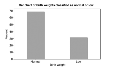
There are many types of bar charts including simple bar charts, stacked bar charts, and comparative side-by-side bar charts. An example of a simple bar chart for the weight classification for babies, which takes on the values normal and low, in the Birth Weight data set is shown in Figure 4.1.
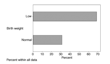
Note that a bar chart represents the category percentages or proportions with bars of height equal to the percentage or proportion of sample observations falling in a particular category. The widths of the bars should be equal and chosen so that an appealing chart is produced. Bar charts may be drawn with either horizontal or vertical bars, and the bars in a bar chart may or may not be separated by a gap. An example of a bar chart with horizontal bars is given in Figure $4.2$ for the weight classification of babies in the Birth Weight data set.
In creating a bar chart it is important that
- the proportions or percentages in each bar can be easily determined to make the bar chart easier to read and interpret.
- the total percentage represented in the bar chart should be 100 since a distribution contains $100 \%$ of the population units.
- the qualities associated with an ordinal variable are listed in the proper relative order! With a nominal variable the order of the categories is not important.
- the bar chart has the axes of the bar chart clearly labeled so that it is clear whether the bars represent a percentage or a proportion.
- the bar chart has either a caption or a title that clearly describes the nature of the bar chart.
生物统计代考
统计代写|生物统计代写biostatistics代考|The Sample Size for Simple and Systematic Random Samples
在简单随机样本或系统随机样本中,为估计均值而对估计误差产生预先指定的界限所需的样本量基于总体中的单位数(ñ),以及总体的近似方差σ2. 此外,鉴于ñ和σ2, 估计平均值所需的样本量μ估计误差有界乙一个简单或系统的随机样本是
n=ñσ2(ñ−1)D+σ2
在哪里D=乙24. 请注意,此公式通常不会返回样本量的整数n; 当公式没有返回样本量的整数时,应将样本量取为下一个最大的整数。
例 3.11
假设一个简单的随机样本将从人口中抽取ñ=5000方差为的单位σ2=50. 如果平均值估计误差的界限应该是乙=1.5,则从该总体中选择的简单随机样本所需的样本量为
n=5000(50)4999(1.524)+50=87.35
自从87.35单位不能被抽样,应该使用的样本量是n=88. 还,n=当估计平均值的估计误差的期望界限为乙=1.5. 在这种情况下,系统随机样本将是 56 个系统随机样本中的 1 个,因为500088≈56.
在许多研究项目中,ñ或者σ2往往是未知的。当ñ或者σ2是未知的,确定样本大小以产生一个简单随机样本的估计误差界限的公式仍然可以使用,只要近似值ñ和σ2可用。在这种情况下,得到的样本量将产生一个接近于估计误差的界限乙提供的近似值ñ和σ2是相当准确的。
被抽样单位在总体中的比例为n/ñ,称为抽样比例。当无法合理地对总体规模做出粗略的猜测,但很明显抽样比例会小于5%,则需要一个用于确定样本量的替代公式。在这种情况下,简单随机样本或系统随机样本所需的样本量限制了估计误差乙估计平均值大约是
n=4σ2乙2
统计代写|生物统计代写biostatistics代考|The Sample Size for a Stratified Random Sample
回想一下,分层随机样本只是从目标人群的亚群中选择的简单随机样本的集合。在分层随机样本中,有两个样本量考虑,即总体样本量n和分配n地层上的单位。当有ķ分层,分层样本大小将表示为n1,n2,n3,…,nķ,其中第 1 层中要采样的数量是n1,第 2 层中要采样的数量为n2, 等等。
有几种不同的方法可以确定总体样本量及其在分层随机样本中的分配。尤其是比例分配和最优分配是两种常用的分配方案。在这两个分配计划的讨论中,将假设目标人群有ķ地层,ñ单位,和ñj是单元的数量j第层。
分层随机样本中使用的样本量和样本的最有效分配将取决于几个因素,包括每个层内的可变性、每个层中目标人群的比例以及与抽样相关的成本来自地层的单位。让σ一世是标准差一世第层,在一世=ñ一世/ñ目标人群的比例一世第层,C0抽样的初始成本,C一世获得观察的成本一世th 层,和C是抽样的总成本。那么,分层随机样本的抽样成本为
C=C0+C1n1+C2n2+⋯+Cķnķ
确定分层随机样本的样本量的过程需要首先确定样本的分配。样本量的分配n超过ķ分层基于由表示的抽样比例在1,在2,…在ķ. 一旦抽样比例和总体样本量n已经确定,一世第层样本量为n一世=n×在一世.
分层随机样本的最简单分配计划是比例分配,它使抽样比例与分层大小成比例。因此,在比例分配中,一世第 th 层等于第 i 层中人口的比例。即,抽样比例为一世第层是
在一世=ñ一世ñ
基于比例分配的分层随机样本的总样本量,估计平均值的估计误差为乙是
n=ñ1σ12+ñ2σ22+⋯+ñķσķ2ñ[乙24]+1ñ(ñ1σ12+ñ2σ22+⋯+ñķσķ2)
将从中选择的简单随机样本的样本量一世根据比例分配的第层是
n×在一世=n×ñ一世ñ
统计代写|生物统计代写biostatistics代考|Bar and Pie Charts
在定性或离散数据的情况下,最常用于总结观察样本中数据的图形统计是条形图和饼图,因为
定性变量分布的重要参数是人口比例。因此,对于定性变量,样本比例是将显示在条形图或饼图中的值。
在第 2 章中,定性变量的分布通常以条形图的形式呈现,其中条形的高度表示具有该变量所具有的每种质量的总体的比例或百分比。对于观察到的样本,条形图可用于表示变量所具有的每种质量的样本比例或百分比,并可用于对变量的总体分布进行统计推断。
有许多类型的条形图,包括简单条形图、堆叠条形图和比较并排条形图。图 4.1 显示了婴儿体重分类的简单条形图示例,它在出生体重数据集中采用正常值和低值。
请注意,条形图表示类别百分比或比例,高度条的高度等于样本观测值落入特定类别的百分比或比例。条形的宽度应相等并进行选择,以便生成吸引人的图表。条形图可以用水平或垂直条形绘制,条形图中的条形可能会或可能不会被间隙分隔。图 1 给出了一个带有水平条的条形图示例4.2用于出生体重数据集中婴儿的体重分类。
在创建条形图时,重要的是
- 可以轻松确定每个条形中的比例或百分比,以使条形图更易于阅读和解释。
- 条形图中表示的总百分比应为 100,因为分布包含100%人口单位。
- 与序数变量相关的质量以正确的相对顺序列出!对于名义变量,类别的顺序并不重要。
- 条形图清楚地标记了条形图的轴,以便清楚条形是代表百分比还是比例。
- 条形图具有清楚地描述条形图性质的标题或标题。

统计代写请认准statistics-lab™. statistics-lab™为您的留学生涯保驾护航。
金融工程代写
金融工程是使用数学技术来解决金融问题。金融工程使用计算机科学、统计学、经济学和应用数学领域的工具和知识来解决当前的金融问题,以及设计新的和创新的金融产品。
非参数统计代写
非参数统计指的是一种统计方法,其中不假设数据来自于由少数参数决定的规定模型;这种模型的例子包括正态分布模型和线性回归模型。
广义线性模型代考
广义线性模型(GLM)归属统计学领域,是一种应用灵活的线性回归模型。该模型允许因变量的偏差分布有除了正态分布之外的其它分布。
术语 广义线性模型(GLM)通常是指给定连续和/或分类预测因素的连续响应变量的常规线性回归模型。它包括多元线性回归,以及方差分析和方差分析(仅含固定效应)。
有限元方法代写
有限元方法(FEM)是一种流行的方法,用于数值解决工程和数学建模中出现的微分方程。典型的问题领域包括结构分析、传热、流体流动、质量运输和电磁势等传统领域。
有限元是一种通用的数值方法,用于解决两个或三个空间变量的偏微分方程(即一些边界值问题)。为了解决一个问题,有限元将一个大系统细分为更小、更简单的部分,称为有限元。这是通过在空间维度上的特定空间离散化来实现的,它是通过构建对象的网格来实现的:用于求解的数值域,它有有限数量的点。边界值问题的有限元方法表述最终导致一个代数方程组。该方法在域上对未知函数进行逼近。[1] 然后将模拟这些有限元的简单方程组合成一个更大的方程系统,以模拟整个问题。然后,有限元通过变化微积分使相关的误差函数最小化来逼近一个解决方案。
tatistics-lab作为专业的留学生服务机构,多年来已为美国、英国、加拿大、澳洲等留学热门地的学生提供专业的学术服务,包括但不限于Essay代写,Assignment代写,Dissertation代写,Report代写,小组作业代写,Proposal代写,Paper代写,Presentation代写,计算机作业代写,论文修改和润色,网课代做,exam代考等等。写作范围涵盖高中,本科,研究生等海外留学全阶段,辐射金融,经济学,会计学,审计学,管理学等全球99%专业科目。写作团队既有专业英语母语作者,也有海外名校硕博留学生,每位写作老师都拥有过硬的语言能力,专业的学科背景和学术写作经验。我们承诺100%原创,100%专业,100%准时,100%满意。
随机分析代写
随机微积分是数学的一个分支,对随机过程进行操作。它允许为随机过程的积分定义一个关于随机过程的一致的积分理论。这个领域是由日本数学家伊藤清在第二次世界大战期间创建并开始的。
时间序列分析代写
随机过程,是依赖于参数的一组随机变量的全体,参数通常是时间。 随机变量是随机现象的数量表现,其时间序列是一组按照时间发生先后顺序进行排列的数据点序列。通常一组时间序列的时间间隔为一恒定值(如1秒,5分钟,12小时,7天,1年),因此时间序列可以作为离散时间数据进行分析处理。研究时间序列数据的意义在于现实中,往往需要研究某个事物其随时间发展变化的规律。这就需要通过研究该事物过去发展的历史记录,以得到其自身发展的规律。
回归分析代写
多元回归分析渐进(Multiple Regression Analysis Asymptotics)属于计量经济学领域,主要是一种数学上的统计分析方法,可以分析复杂情况下各影响因素的数学关系,在自然科学、社会和经济学等多个领域内应用广泛。
MATLAB代写
MATLAB 是一种用于技术计算的高性能语言。它将计算、可视化和编程集成在一个易于使用的环境中,其中问题和解决方案以熟悉的数学符号表示。典型用途包括:数学和计算算法开发建模、仿真和原型制作数据分析、探索和可视化科学和工程图形应用程序开发,包括图形用户界面构建MATLAB 是一个交互式系统,其基本数据元素是一个不需要维度的数组。这使您可以解决许多技术计算问题,尤其是那些具有矩阵和向量公式的问题,而只需用 C 或 Fortran 等标量非交互式语言编写程序所需的时间的一小部分。MATLAB 名称代表矩阵实验室。MATLAB 最初的编写目的是提供对由 LINPACK 和 EISPACK 项目开发的矩阵软件的轻松访问,这两个项目共同代表了矩阵计算软件的最新技术。MATLAB 经过多年的发展,得到了许多用户的投入。在大学环境中,它是数学、工程和科学入门和高级课程的标准教学工具。在工业领域,MATLAB 是高效研究、开发和分析的首选工具。MATLAB 具有一系列称为工具箱的特定于应用程序的解决方案。对于大多数 MATLAB 用户来说非常重要,工具箱允许您学习和应用专业技术。工具箱是 MATLAB 函数(M 文件)的综合集合,可扩展 MATLAB 环境以解决特定类别的问题。可用工具箱的领域包括信号处理、控制系统、神经网络、模糊逻辑、小波、仿真等。