如果你也在 怎样代写生物统计学Biostatistics这个学科遇到相关的难题,请随时右上角联系我们的24/7代写客服。
生物统计学是将统计技术应用于健康相关领域的科学研究,包括医学、生物学和公共卫生,并开发新的工具来研究这些领域。
statistics-lab™ 为您的留学生涯保驾护航 在代写生物统计学Biostatistics方面已经树立了自己的口碑, 保证靠谱, 高质且原创的统计Statistics代写服务。我们的专家在代写生物统计学Biostatistics方面经验极为丰富,各种代写生物统计学Biostatistics相关的作业也就用不着说。
我们提供的生物统计学Biostatistics及其相关学科的代写,服务范围广, 其中包括但不限于:
- Statistical Inference 统计推断
- Statistical Computing 统计计算
- Advanced Probability Theory 高等楖率论
- Advanced Mathematical Statistics 高等数理统计学
- (Generalized) Linear Models 广义线性模型
- Statistical Machine Learning 统计机器学习
- Longitudinal Data Analysis 纵向数据分析
- Foundations of Data Science 数据科学基础
统计代写|生物统计学作业代写Biostatistics代考|Mean and Variance
As seen in Sections $3.3$ and $3.4$, a probability density function $f$ is defined so that:
(a) $f(k)=\operatorname{Pr}(X=k)$ in the discrete case
(b) $f(x) d x=\operatorname{Pr}(x \leq X \leq x+d x)$ in the continuous case
For a continuous distribution, such as the normal distribution, the mean $\mu$ and variance $\sigma^{2}$ are calculated from:
(a) $\mu=\int x f(x) d x$
(b) $\sigma^{2}=\int(x-\mu)^{2} f(x) d x$
For a discrete distribution, such as the binomial distribution or Poisson distribution, the mean $\mu$ and variance $\sigma^{2}$ are calculated from:
(a) $\mu=\sum x f(x)$
(b) $\sigma^{2}=\sum(x-\mu)^{2} f(x)$
For example, we have for the binomial distribution,
$$
\begin{aligned}
\mu &=n p \
\sigma^{2} &=n p(1-p)
\end{aligned}
$$
and for the Poisson distribution,
$$
\begin{aligned}
\mu &=\theta \
\sigma^{2} &=\theta
\end{aligned}
$$
统计代写|生物统计学作业代写Biostatistics代考|Pair-Matched Case–Control Study
Data from epidemiologic studies may come from various sources, the two fundamental designs being retrospective and prospective (or cohort). Retrospective studies gather past data from selected cases (diseased individuals) and controls (nondiseased individuals) to determine differences, if any, in the exposure to a suspected risk factor. They are commonly referred to as case-control studies. Cases of a specific disease, such as lung cancer, are ascertained as they arise from population-based disease registers or lists of hospital admissions, and controls are sampled either as disease-free persons from the population at risk or as hospitalized patients having a diagnosis other than the one under investigation. The advantages of a case-control study are that it is economical and that it is possible to answer research questions relatively quickly because the cases are already available. Suppose that each person in a large population has been classified as exposed or not exposed to a certain factor, and as having or not having some disease. The population may then be enumerated in a $2 \times 2$ table (Table 3.12), with entries being the proportions of the total population.
Using these proportions, the association (if any) between the factor and the disease could be measured by the ratio of risks (or relative risk) of being disease positive for those with or without the factor:
$$
\begin{aligned}
\text { relative risk } &=\frac{P_{1}}{P_{1}+P_{3}} \div \frac{P_{2}}{P_{2}+P_{4}} \
&=\frac{P_{1}\left(P_{2}+P_{4}\right)}{P_{2}\left(P_{1}+P_{3}\right)}
\end{aligned}
$$
since in many (although not all) situations, the proportions of subjects classified as disease positive will be small. That is, $P_{1}$ is small in comparison with $P_{3}$, and $P_{2}$ will be small in comparison with $P_{4}$. In such a case, the relative risk is almost equal to
$$
\begin{aligned}
\theta &=\frac{P_{1} P_{4}}{P_{2} P_{3}} \
&=\frac{P_{1} / P_{3}}{P_{2} / P_{4}}
\end{aligned}
$$
the odds ratio of being disease positive, or
$$
=\frac{P_{1} / P_{2}}{P_{3} / P_{4}}
$$
the odds ratio of being exposed. This justifies the use of an odds ratio to determine differences, if any, in the exposure to a suspected risk factor.
As a technique to control confounding factors in a designed study, individual cases are matched, often one to one, to a set of controls chosen to have similar values for the important confounding variables. The simplest example of pair-matched data occurs with a single binary exposure (e.g., smoking versus nonsmoking). The data for outcomes can be represented by a $2 \times 2$ table (Table 3.13) where $(+,-)$ denotes (exposed, unexposed).
For example, $n_{10}$ denotes the number of pairs where the case is exposed, but the matched control is unexposed. The most suitable statistical model for making inferences about the odds ratio $\theta$ is to use the conditional probability of the number of exposed cases among the discordant pairs. Given $n=n_{10}+n_{01}$ being fixed, it can be seen that $n_{10}$ has $B(n, p)$, where
$$
p=\frac{\theta}{1+\theta}
$$
统计代写|生物统计学作业代写Biostatistics代考|NOTES ON COMPUTATIONS
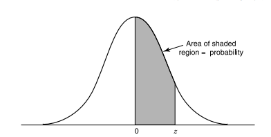
In Sections $1.4$ and $2.5$ we covered basic techniques for Microsoft’s Excel: how to open/form a spreadsheet, save it, retrieve it, and perform certain descriptive statistical tasks. Topics included data-entry steps, such as select and drag, use of formula bar, bar and pie charts, histograms, calculations of descritive statistics such as mean and standard deviation, and calculation of a coefficient of correlation. In this short section we focus on probability models related to the calculation of areas under density curves, especially normal curves and $t$ curves.
Normal Curves The first two steps are the same as in obtaining descriptive statistics (but no data are needed now): (1) click the paste function icon, $\mathrm{f}^{*}$, and (2) click Statistical. Among the functions available, two are related to normal curves: NORMDIST and NORMINV. Excel provides needed information for any normal distribution, not just the standard normal distribution as in Appendix B. Upon selecting either one of the two functions above, a box appears asking you to provide (1) the mean $\mu,(2)$ the standard deviation $\sigma$, and (3) in the last row, marked cumulative, to enter TRUE (there is a choice $F A L S E$, but you do not need that). The answer will appear in a preselected cell.
- NORMDIST gives the area under the normal curve (with mean and variance provided) all the way from the far-left side (minus infinity) to the value $x$ that you have to specify. For example, if you specify $\mu=0$ and $\sigma=1$, the return is the area under the standard normal curve up to the point specified (which is the same as the number from Appendix B plus $0.5)$.
- NORMINV performs the inverse process, where you provide the area under the normal curve (a number between 0 and 1), together with the mean $\mu$ and standard deviation $\sigma$, and requests the point $x$ on the horizontal axis so that the area under that normal curve from the far-left side (minus infinity) to the value $x$ is equal to the number provided between 0 and 1. For example, if you put in $\mu=0, \sigma=1$, and probability $=0.975$, the return is $1.96$; unlike Appendix $B$, if you want a number in the right tail of the curve, the input probability should be a number greater than $0.5$.
The $t$ Curves: Procedures TDIST and TINV We want to learn how to find the areas under the normal curves so that we can determine the $p$ values for statistical tests (a topic starting in Chapter 5). Another popular family in this category is the $t$ distributions, which begin with the same first two steps: (1) click the paste function icon, $\mathrm{f}^{*}$, and (2) click Statistical. Among the functions available, two related to the $t$ distributions are TDIST and TINV. Similar to the case of NORMDIST and NORMINV, TDIST gives the area under the $t$ curve, and TINV performs the inverse process where you provide the area under the curve and request point $x$ on the horizontal axis. In each case you have to provide the degrees of freedom. In addition, in the last row, marked with tails, enter: - (Tails=) $I$ if you want one-sided
- (Tails $=) 2$ if you want $t$ wo-sided
(More details on the concepts of one- and two-sided areas are given in Chapter
5.) For example: - Example 1: If you enter $(\mathrm{x}=) 2.73,($ deg freedom $=) 18$, and, (Tails $=) 1$, you’re requesting the area under a $t$ curve with 18 degrees of freedom and to the right of $2.73$ (i.e., right tail); the answer is $0.00687$.
- Example 2: If you enter $(\mathrm{x}=) 2.73$, (deg freedom $=) 18$, and (Tails $=) 2$, you’re requesting the area under a $t$ curve with 18 degrees of freedom and to the right of $2.73$ and to the left of $-2.73$ (i.e., both right and left tails); the answer is $0.01374$, which is twice the previous answer of $0.00687$.
生物统计代写
统计代写|生物统计学作业代写Biostatistics代考|Mean and Variance
如部分所示3.3和3.4, 一个概率密度函数F被定义为:
(a)F(ķ)=公关(X=ķ)在离散情况下
(b)F(X)dX=公关(X≤X≤X+dX)在连续情况下
对于连续分布,例如正态分布,均值μ和方差σ2由以下计算得出:
(a)μ=∫XF(X)dX
(二)σ2=∫(X−μ)2F(X)dX
对于离散分布,例如二项分布或泊松分布,均值μ和方差σ2计算自:
(一种)μ=∑XF(X)
(二)σ2=∑(X−μ)2F(X)
例如,对于二项分布,我们有,
μ=np σ2=np(1−p)
对于泊松分布,
μ=θ σ2=θ
统计代写|生物统计学作业代写Biostatistics代考|Pair-Matched Case–Control Study
流行病学研究的数据可能来自各种来源,两种基本设计是回顾性和前瞻性(或队列)。回顾性研究从选定的病例(患病个体)和对照(非患病个体)收集过去的数据,以确定暴露于疑似风险因素的差异(如果有)。它们通常被称为病例对照研究。特定疾病(例如肺癌)的病例是从基于人群的疾病登记册或住院名单中确定的,并且对照从处于危险中的人群中作为无病人群或作为确诊的住院患者进行抽样除了正在调查的那个。病例对照研究的优点是经济实惠,并且可以相对快速地回答研究问题,因为病例已经可用。假设大量人群中的每个人都被分类为暴露于或未暴露于某种因素,以及患有或不患有某种疾病。然后可以在一个2×2表(表 3.12),条目是总人口的比例。
使用这些比例,因素和疾病之间的关联(如果有的话)可以通过有或没有因素的人疾病阳性的风险(或相对风险)的比率来衡量: 相对风险 =磷1磷1+磷3÷磷2磷2+磷4 =磷1(磷2+磷4)磷2(磷1+磷3)
因为在许多(尽管不是全部)情况下,被归类为疾病阳性的受试者的比例很小。那是,磷1与磷3, 和磷2与磷4. 在这种情况下,相对风险几乎等于
θ=磷1磷4磷2磷3 =磷1/磷3磷2/磷4
疾病阳性的优势比,或
=磷1/磷2磷3/磷4
暴露的几率。这证明了使用优势比来确定暴露于可疑风险因素的差异(如果有)是合理的。
作为在设计研究中控制混杂因素的一种技术,个别案例通常一对一地匹配到一组选择为重要混杂变量具有相似值的控制。配对数据的最简单示例发生在单个二元暴露(例如,吸烟与不吸烟)中。结果的数据可以表示为2×2表(表 3.13) 其中(+,−)表示(曝光,未曝光)。
例如,n10表示案例暴露但匹配的控制未暴露的对数。最适合推断优势比的统计模型θ是使用不一致对中暴露病例数的条件概率。给定n=n10+n01被修复,可以看出n10拥有乙(n,p), 在哪里
p=θ1+θ
统计代写|生物统计学作业代写Biostatistics代考|NOTES ON COMPUTATIONS
在部分1.4和2.5我们介绍了 Microsoft Excel 的基本技术:如何打开/形成电子表格、保存、检索它以及执行某些描述性统计任务。主题包括数据输入步骤,例如选择和拖动、公式栏、条形图和饼图的使用、直方图、描述性统计数据(例如均值和标准差)的计算以及相关系数的计算。在这个简短的部分中,我们将重点关注与密度曲线下面积计算相关的概率模型,尤其是正态曲线和吨曲线。
正态曲线 前两步与获取描述性统计相同(但现在不需要数据):(1)点击粘贴功能图标,F∗,和 (2) 单击统计。在可用的函数中,有两个与正态曲线相关:NORMDIST 和 NORMINV。Excel 提供任何正态分布所需的信息,而不仅仅是附录 B 中的标准正态分布。选择上述两个函数中的任何一个后,会出现一个框,要求您提供 (1) 平均值μ,(2)标准差σ,和(3)在最后一行,标记为累积,输入TRUE(有一个选择F一种大号小号和,但你不需要那个)。答案将出现在预选的单元格中。
- NORMDIST 给出从最左侧(负无穷大)一直到值的正态曲线下面积(提供均值和方差)X您必须指定。例如,如果您指定μ=0和σ=1,返回是标准正态曲线下到指定点的面积(与附录 B 中的数字相同加上0.5).
- NORMINV 执行逆过程,您提供正态曲线下的面积(0 到 1 之间的数字)以及平均值μ和标准差σ, 并请求点X在水平轴上,使得从最左侧(负无穷大)到该值的正态曲线下的面积X等于在 0 和 1 之间提供的数字。例如,如果您输入μ=0,σ=1, 和概率=0.975,回报是1.96; 不同于附录乙,如果你想在曲线的右尾有一个数字,输入概率应该是一个大于0.5.
这吨曲线:过程 TDIST 和 TINV 我们想学习如何找到正态曲线下的区域,以便我们可以确定p统计检验的值(从第 5 章开始的主题)。此类别中另一个受欢迎的家庭是吨发行版,前两个步骤相同:(1)单击粘贴功能图标,F∗,和 (2) 单击统计。在可用的功能中,有两个与吨分布是 TDIST 和 TINV。与 NORMDIST 和 NORMINV 的情况类似,TDIST 给出了吨曲线,TINV 执行逆过程,您提供曲线下面积和请求点X在水平轴上。在每种情况下,您都必须提供自由度。此外,在最后一行标有尾巴的地方,输入: - (尾巴=)一世如果你想要一面
- (尾巴=)2如果你想吨双面
(有关单面和双面区域概念的更多详细信息,请参见第
5 章。)例如: - 示例 1:如果您输入(X=)2.73,(你自由=)18, 并且, (尾巴=)1,您正在请求 a 下的区域吨具有 18 个自由度和右侧的曲线2.73(即右尾);答案是0.00687.
- 示例 2:如果您输入(X=)2.73,(你的自由=)18, 和 (尾巴=)2,您正在请求 a 下的区域吨具有 18 个自由度和右侧的曲线2.73和左边−2.73(即左右尾巴);答案是0.01374,这是先前答案的两倍0.00687.

统计代写请认准statistics-lab™. statistics-lab™为您的留学生涯保驾护航。统计代写|python代写代考
随机过程代考
在概率论概念中,随机过程是随机变量的集合。 若一随机系统的样本点是随机函数,则称此函数为样本函数,这一随机系统全部样本函数的集合是一个随机过程。 实际应用中,样本函数的一般定义在时间域或者空间域。 随机过程的实例如股票和汇率的波动、语音信号、视频信号、体温的变化,随机运动如布朗运动、随机徘徊等等。
贝叶斯方法代考
贝叶斯统计概念及数据分析表示使用概率陈述回答有关未知参数的研究问题以及统计范式。后验分布包括关于参数的先验分布,和基于观测数据提供关于参数的信息似然模型。根据选择的先验分布和似然模型,后验分布可以解析或近似,例如,马尔科夫链蒙特卡罗 (MCMC) 方法之一。贝叶斯统计概念及数据分析使用后验分布来形成模型参数的各种摘要,包括点估计,如后验平均值、中位数、百分位数和称为可信区间的区间估计。此外,所有关于模型参数的统计检验都可以表示为基于估计后验分布的概率报表。
广义线性模型代考
广义线性模型(GLM)归属统计学领域,是一种应用灵活的线性回归模型。该模型允许因变量的偏差分布有除了正态分布之外的其它分布。
statistics-lab作为专业的留学生服务机构,多年来已为美国、英国、加拿大、澳洲等留学热门地的学生提供专业的学术服务,包括但不限于Essay代写,Assignment代写,Dissertation代写,Report代写,小组作业代写,Proposal代写,Paper代写,Presentation代写,计算机作业代写,论文修改和润色,网课代做,exam代考等等。写作范围涵盖高中,本科,研究生等海外留学全阶段,辐射金融,经济学,会计学,审计学,管理学等全球99%专业科目。写作团队既有专业英语母语作者,也有海外名校硕博留学生,每位写作老师都拥有过硬的语言能力,专业的学科背景和学术写作经验。我们承诺100%原创,100%专业,100%准时,100%满意。
机器学习代写
随着AI的大潮到来,Machine Learning逐渐成为一个新的学习热点。同时与传统CS相比,Machine Learning在其他领域也有着广泛的应用,因此这门学科成为不仅折磨CS专业同学的“小恶魔”,也是折磨生物、化学、统计等其他学科留学生的“大魔王”。学习Machine learning的一大绊脚石在于使用语言众多,跨学科范围广,所以学习起来尤其困难。但是不管你在学习Machine Learning时遇到任何难题,StudyGate专业导师团队都能为你轻松解决。
多元统计分析代考
基础数据: $N$ 个样本, $P$ 个变量数的单样本,组成的横列的数据表
变量定性: 分类和顺序;变量定量:数值
数学公式的角度分为: 因变量与自变量
时间序列分析代写
随机过程,是依赖于参数的一组随机变量的全体,参数通常是时间。 随机变量是随机现象的数量表现,其时间序列是一组按照时间发生先后顺序进行排列的数据点序列。通常一组时间序列的时间间隔为一恒定值(如1秒,5分钟,12小时,7天,1年),因此时间序列可以作为离散时间数据进行分析处理。研究时间序列数据的意义在于现实中,往往需要研究某个事物其随时间发展变化的规律。这就需要通过研究该事物过去发展的历史记录,以得到其自身发展的规律。
回归分析代写
多元回归分析渐进(Multiple Regression Analysis Asymptotics)属于计量经济学领域,主要是一种数学上的统计分析方法,可以分析复杂情况下各影响因素的数学关系,在自然科学、社会和经济学等多个领域内应用广泛。
MATLAB代写
MATLAB 是一种用于技术计算的高性能语言。它将计算、可视化和编程集成在一个易于使用的环境中,其中问题和解决方案以熟悉的数学符号表示。典型用途包括:数学和计算算法开发建模、仿真和原型制作数据分析、探索和可视化科学和工程图形应用程序开发,包括图形用户界面构建MATLAB 是一个交互式系统,其基本数据元素是一个不需要维度的数组。这使您可以解决许多技术计算问题,尤其是那些具有矩阵和向量公式的问题,而只需用 C 或 Fortran 等标量非交互式语言编写程序所需的时间的一小部分。MATLAB 名称代表矩阵实验室。MATLAB 最初的编写目的是提供对由 LINPACK 和 EISPACK 项目开发的矩阵软件的轻松访问,这两个项目共同代表了矩阵计算软件的最新技术。MATLAB 经过多年的发展,得到了许多用户的投入。在大学环境中,它是数学、工程和科学入门和高级课程的标准教学工具。在工业领域,MATLAB 是高效研究、开发和分析的首选工具。MATLAB 具有一系列称为工具箱的特定于应用程序的解决方案。对于大多数 MATLAB 用户来说非常重要,工具箱允许您学习和应用专业技术。工具箱是 MATLAB 函数(M 文件)的综合集合,可扩展 MATLAB 环境以解决特定类别的问题。可用工具箱的领域包括信号处理、控制系统、神经网络、模糊逻辑、小波、仿真等。