如果你也在 怎样代写生物统计学Biostatistics这个学科遇到相关的难题,请随时右上角联系我们的24/7代写客服。
生物统计学是将统计技术应用于健康相关领域的科学研究,包括医学、生物学和公共卫生,并开发新的工具来研究这些领域。
statistics-lab™ 为您的留学生涯保驾护航 在代写生物统计学Biostatistics方面已经树立了自己的口碑, 保证靠谱, 高质且原创的统计Statistics代写服务。我们的专家在代写生物统计学Biostatistics方面经验极为丰富,各种代写生物统计学Biostatistics相关的作业也就用不着说。
我们提供的生物统计学Biostatistics及其相关学科的代写,服务范围广, 其中包括但不限于:
- Statistical Inference 统计推断
- Statistical Computing 统计计算
- Advanced Probability Theory 高等楖率论
- Advanced Mathematical Statistics 高等数理统计学
- (Generalized) Linear Models 广义线性模型
- Statistical Machine Learning 统计机器学习
- Longitudinal Data Analysis 纵向数据分析
- Foundations of Data Science 数据科学基础
统计代写|生物统计学作业代写Biostatistics代考|Frequency Distribution
There is no difficulty if the data set is small, for we can arrange those few numbers and write them, say, in increasing order; the result would be sufficiently clear; Figure $2.1$ is an example. For fairly large data sets, a useful device for summarization is the formation of a frequency table or frequency distribution. This is a table showing the number of observations, called frequency, within certain ranges of values of the variable under investigation. For example, taking the variable to be the age at death, we have the following example; the second column of the table provides the frequencies.
Example 2.1 Table $2.1$ gives the number of deaths by age for the state of Minnesota in $1987 .$
If a data set is to be grouped to form a frequency distribution, difficulties should be recognized, and an efficient strategy is needed for better communication. First, there is no clear-cut rule on the number of intervals or classes. With too many intervals, the data are not summarized enough for a clear visualization of how they are distributed. On the other hand, too few intervals are undesirable because the data are oversummarized, and some of the details of the distribution may be lost. In general, between 5 and 15 intervals are acceptable; of course, this also depends on the number of observations, we can and should use more intervals for larger data sets.
The widths of the intervals must also be decided. Example $2.1$ shows the special case of mortality data, where it is traditional to show infant deaths (deaths of persons who are born live but die before living one year). Without such specific reasons, intervals generally should be of the same width. This common width $w$ may be determined by dividing the range $R$ by $k$, the number of intervals:
$$
w=\frac{R}{k}
$$
where the range $R$ is the difference between the smallest and largest in the data set. In addition, a width should be chosen so that it is convenient to use or easy to recognize, such as a multiple of 5 (or 1 , for example, if the data set has a narrow range). Similar considerations apply to the choice of the beginning of the first interval; it is a convenient number that is low enough for the first interval to include the smallest observation. Finally, care should be taken in deciding in which interval to place an observation falling on one of the interval boundaries. For example, a consistent rule could be made so as to place such an observation in the interval of which the observation in question is the lower limit.
统计代写|生物统计学作业代写Biostatistics代考|Histogram and the Frequency Polygon
A convenient way of displaying a frequency table is by means of a histogram and/or a frequency polygon. A histogram is a diagram in which:
- The horizontal scale represents the value of the variable marked at interval boundaries.
- The vertical scale represents the frequency or relative frequency in each interval (see the exceptions below).
A histogram presents us with a graphic picture of the distribution of measurements. This picture consists of rectangular bars joining each other, one for each interval, as shown in Figure $2.2$ for the data set of Example 2.2. If disjoint intervals are used, such as in Table $2.2$, the horizontal axis is marked with true boundaries. A true boundary is the average of the upper limit of one interval and the lower limit of the next-higher interval. For example, $19.5$ serves as the true upper boundary of the first interval and the true lower boundary for the second interval. In cases where we need to compare the shapes of the histograms representing different data sets, or if intervals are of unequal widths, the height of each rectangular bar should represent the density of the interval, where the interval density is defined by
$$
\text { density }=\frac{\text { relative frequency }(\%)}{\text { interval width }}
$$
The unit for density is percent per unit (of measurement): for example, percent per year. If we graph densities on the vertical axis, the relative frequency is represented by the area of the rectangular bar, and the total area under the histogram is $100 \%$. It may always be a good practice to graph densities on the vertical axis with or without having equal class width; when class widths are
equal, the shape of the histogram looks similar to the graph, with relative frequencies on the vertical axis.
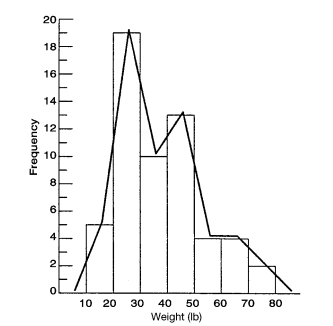
To draw a frequency polygon, we first place a dot at the midpoint of the upper base of each rectangular bar. The points are connected with straight lines. At the ends, the points are connected to the midpoints of the previous and succeeding intervals (these are make-up intervals with zero frequency, where widths are the widths of the first and last intervals, respectively). A frequency polygon so constructed is another way to portray graphically the distribution of a data set (Figure 2.3). The frequency polygon can also be shown without the histogram on the same graph.
The frequency table and its graphical relatives, the histogram and the frequency polygon, have a number of applications, as explained below; the first leads to a research question and the second leads to a new analysis strategy.
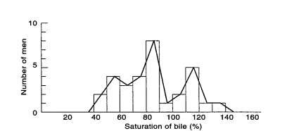
- When data are homogeneous, the table and graphs usually show a unimodal pattern with one peak in the middle part. A bimodal pattern might indicate the possible influence or effect of a certain hidden factor or factors.
统计代写|生物统计学作业代写Biostatistics代考|Cumulative Frequency Graph and Percentiles
Cumulative relative frequency, or cumulative percentage, gives the percentage of persons having a measurement less than or equal to the upper boundary of the class interval. Data from Table $2.2$ for the distribution of weights of 57 children are reproduced and supplemented with a column for cumulative relative frequency in Table 2.6. This last column is easy to form; you do it by successively accumulating the relative frequencies of each of the various intervals. In the table the cumulative percentage for the first three intervals is
$$
8.8+33.3+17.5=59.6
$$
and we can say that $59.6 \%$ of the children in the data set have a weight of $39.5$ $\mathrm{lb}$ or less. Or, as another example, $96.4 \%$ of children weigh $69.5 \mathrm{lb}$ or less, and so on.
The cumulative relative frequency can be presented graphically as in Figure 2.6. This type of curve is called a cumulative frequency graph. To construct such a graph, we place a point with a horizontal axis marked at the upper class boundary and a vertical axis marked at the corresponding cumulative frequency. Each point represents the cumulative relative frequency and the points are connected with straight lines. At the left end it is connected to the lower boundary of the first interval. If disjoint intervals such as
$$
\begin{aligned}
&10-19 \
&20-29 \
&\text { etc. } .
\end{aligned}
$$
are used, points are placed at the true boundaries.
The cumulative percentages and their graphical representation, the cumulative frequency graph, have a number of applications. When two cumulative frequency graphs, representing two different data sets, are placed on the same
graph, they provide a rapid visual comparison without any need to compare individual intervals. Figure $2.7$ gives such a comparison of family incomes using data of Example $2.5$.
The cumulative frequency graph provides a class of important statistics known as percentiles or percentile scores. The 90 th percentile, for example, is the numerical value that exceeds $90 \%$ of the values in the data set and is exceeded by only $10 \%$ of them. Or, as another example, the 80 th percentile is that numerical value that exceeds $80 \%$ of the values contained in the data set and is exceeded by $20 \%$ of them, and so on. The 50 th percentile is commonly
called the median. In Figure $2.7$ the median family income in 1983 for nonwhites was about $\$ 17,500$, compared to a median of about $\$ 22,000$ for white families. To get the median, we start at the $50 \%$ point on the vertical axis and go horizontally until meeting the cumulative frequency graph; the projection of this intersection on the horizontal axis is the median. Other percentiles are obtained similarly.
The cumulative frequency graph also provides an important application in the formation of health norms (see Figure $2.8$ ) for the monitoring of physical progress (weight and height) of infants and children. Here, the same percentiles, say the 90 th, of weight or height of groups of different ages are joined by a curve.
生物统计代写
统计代写|生物统计学作业代写Biostatistics代考|Frequency Distribution
如果数据集很小,也没有什么困难,因为我们可以把这几个数字排列起来,比如按升序写;结果将足够清楚;数字2.1是一个例子。对于相当大的数据集,一个有用的汇总方法是形成频率表或频率分布。这是一个表格,显示了在所调查变量的某些值范围内的观察次数(称为频率)。例如,将变量作为死亡年龄,我们有以下示例;表的第二列提供了频率。
示例 2.1 表2.1给出明尼苏达州按年龄划分的死亡人数1987.
如果要将数据集分组以形成频率分布,则应认识到困难,并且需要有效的策略以更好地进行通信。首先,对于区间或类的数量没有明确的规则。如果间隔太多,则数据的汇总不足以清晰地显示它们的分布方式。另一方面,太少的间隔是不可取的,因为数据被过度汇总,并且可能会丢失一些分布的细节。一般来说,5 到 15 个间隔是可以接受的;当然,这也取决于观察的数量,我们可以而且应该为更大的数据集使用更多的区间。
间隔的宽度也必须确定。例子2.1显示死亡率数据的特殊情况,传统上显示婴儿死亡(出生时活着但未满一年就死亡的人的死亡)。如果没有这些具体原因,间隔通常应该具有相同的宽度。这个共同的宽度在可以通过划分范围来确定R经过ķ,区间数:
在=Rķ
范围在哪里R是数据集中最小和最大之间的差异。此外,宽度应选择方便使用或易于识别,例如 5 的倍数(或 1,例如,如果数据集范围较窄)。类似的考虑适用于第一个间隔开始的选择;这是一个方便的数字,它足够低,可以让第一个间隔包含最小的观察值。最后,在决定将观测值放置在哪个区间边界上时,应小心谨慎。例如,可以制定一致的规则,以便将这样的观察置于所讨论的观察为下限的区间中。
统计代写|生物统计学作业代写Biostatistics代考|Histogram and the Frequency Polygon
显示频率表的一种方便方式是通过直方图和/或频率多边形。直方图是一种图表,其中:
- 水平刻度表示在区间边界处标记的变量的值。
- 垂直刻度表示每个间隔中的频率或相对频率(请参阅下面的例外情况)。
直方图向我们展示了测量分布的图形。这张图片由相互连接的矩形条组成,每个间隔一个,如图2.2对于示例 2.2 的数据集。如果使用不相交的区间,例如在表中2.2,横轴标有真实边界。真正的边界是一个区间的上限和下一个更高区间的下限的平均值。例如,19.5用作第一个区间的真实上边界和第二个区间的真实下边界。在我们需要比较代表不同数据集的直方图形状的情况下,或者如果区间的宽度不相等,则每个矩形条的高度应该代表区间的密度,其中区间密度定义为
密度 = 相对频率 (%) 间隔宽度
密度的单位是每单位(测量)的百分比:例如,每年的百分比。如果我们在纵轴上绘制密度图,则相对频率由矩形条的面积表示,直方图下的总面积为100%. 在具有或不具有相等类宽度的情况下,在垂直轴上绘制密度图可能总是一个好习惯;当班级宽度为
相等,直方图的形状看起来与图表相似,相对频率在垂直轴上。
为了绘制频率多边形,我们首先在每个矩形条的上底的中点放置一个点。这些点用直线连接。在末端,这些点连接到前一个和后一个区间的中点(这些是零频率的补充区间,其中宽度分别是第一个和最后一个区间的宽度)。如此构造的频率多边形是另一种以图形方式描绘数据集分布的方式(图 2.3)。频率多边形也可以在没有直方图的情况下显示在同一图表上。
频率表及其相关图形、直方图和频率多边形有多种应用,如下所述;第一个引出一个研究问题,第二个引出一个新的分析策略。
- 当数据是同质的时,表格和图表通常显示一个单峰模式,中间有一个峰。双峰模式可能表明某个或多个隐藏因素的可能影响或效果。
统计代写|生物统计学作业代写Biostatistics代考|Cumulative Frequency Graph and Percentiles
累积相对频率或累积百分比给出了测量值小于或等于类区间上边界的人的百分比。表中的数据2.2对于 57 名儿童的体重分布,在表 2.6 中复制并补充了累积相对频率列。最后一列很容易形成;您可以通过连续累积每个不同间隔的相对频率来做到这一点。在表中,前三个间隔的累积百分比是
8.8+33.3+17.5=59.6
我们可以说59.6%数据集中的孩子的权重为39.5 lb或更少。或者,作为另一个例子,96.4%的孩子称重69.5lb或更少,等等。
累积相对频率可以用图形表示,如图 2.6 所示。这种类型的曲线称为累积频率图。为了构建这样的图,我们放置一个点,其水平轴标记在上层边界,垂直轴标记在相应的累积频率处。每个点代表累积的相对频率,并用直线连接。在左端,它连接到第一个区间的下边界。如果不相交的间隔,例如
10−19 20−29 等等 .
被使用时,点被放置在真正的边界上。
累积百分比及其图形表示,累积频率图,有许多应用。当代表两个不同数据集的两个累积频率图放在同一个
图表,它们提供了快速的视觉比较,而无需比较各个间隔。数字2.7使用示例数据对家庭收入进行了这样的比较2.5.
累积频率图提供了一类重要的统计数据,称为百分位数或百分位数分数。例如,第 90 个百分位数是超过90%数据集中的值,仅超过10%其中。或者,作为另一个例子,第 80 个百分位数是超过80%包含在数据集中的值并超过20%其中,等等。第 50 个百分位通常是
称为中位数。如图2.71983 年非白人的家庭收入中位数约为$17,500, 与大约的中位数相比$22,000对于白人家庭。为了得到中位数,我们从50%点在垂直轴上,然后水平走,直到遇到累积频率图;这个交点在横轴上的投影就是中位数。其他百分位数以类似方式获得。
累积频率图在健康规范的形成中也提供了重要的应用(见图2.8) 用于监测婴儿和儿童的身体进步(体重和身高)。在这里,不同年龄组的体重或身高的相同百分位数(例如第 90 个百分位数)由一条曲线连接起来。

统计代写请认准statistics-lab™. statistics-lab™为您的留学生涯保驾护航。统计代写|python代写代考
随机过程代考
在概率论概念中,随机过程是随机变量的集合。 若一随机系统的样本点是随机函数,则称此函数为样本函数,这一随机系统全部样本函数的集合是一个随机过程。 实际应用中,样本函数的一般定义在时间域或者空间域。 随机过程的实例如股票和汇率的波动、语音信号、视频信号、体温的变化,随机运动如布朗运动、随机徘徊等等。
贝叶斯方法代考
贝叶斯统计概念及数据分析表示使用概率陈述回答有关未知参数的研究问题以及统计范式。后验分布包括关于参数的先验分布,和基于观测数据提供关于参数的信息似然模型。根据选择的先验分布和似然模型,后验分布可以解析或近似,例如,马尔科夫链蒙特卡罗 (MCMC) 方法之一。贝叶斯统计概念及数据分析使用后验分布来形成模型参数的各种摘要,包括点估计,如后验平均值、中位数、百分位数和称为可信区间的区间估计。此外,所有关于模型参数的统计检验都可以表示为基于估计后验分布的概率报表。
广义线性模型代考
广义线性模型(GLM)归属统计学领域,是一种应用灵活的线性回归模型。该模型允许因变量的偏差分布有除了正态分布之外的其它分布。
statistics-lab作为专业的留学生服务机构,多年来已为美国、英国、加拿大、澳洲等留学热门地的学生提供专业的学术服务,包括但不限于Essay代写,Assignment代写,Dissertation代写,Report代写,小组作业代写,Proposal代写,Paper代写,Presentation代写,计算机作业代写,论文修改和润色,网课代做,exam代考等等。写作范围涵盖高中,本科,研究生等海外留学全阶段,辐射金融,经济学,会计学,审计学,管理学等全球99%专业科目。写作团队既有专业英语母语作者,也有海外名校硕博留学生,每位写作老师都拥有过硬的语言能力,专业的学科背景和学术写作经验。我们承诺100%原创,100%专业,100%准时,100%满意。
机器学习代写
随着AI的大潮到来,Machine Learning逐渐成为一个新的学习热点。同时与传统CS相比,Machine Learning在其他领域也有着广泛的应用,因此这门学科成为不仅折磨CS专业同学的“小恶魔”,也是折磨生物、化学、统计等其他学科留学生的“大魔王”。学习Machine learning的一大绊脚石在于使用语言众多,跨学科范围广,所以学习起来尤其困难。但是不管你在学习Machine Learning时遇到任何难题,StudyGate专业导师团队都能为你轻松解决。
多元统计分析代考
基础数据: $N$ 个样本, $P$ 个变量数的单样本,组成的横列的数据表
变量定性: 分类和顺序;变量定量:数值
数学公式的角度分为: 因变量与自变量
时间序列分析代写
随机过程,是依赖于参数的一组随机变量的全体,参数通常是时间。 随机变量是随机现象的数量表现,其时间序列是一组按照时间发生先后顺序进行排列的数据点序列。通常一组时间序列的时间间隔为一恒定值(如1秒,5分钟,12小时,7天,1年),因此时间序列可以作为离散时间数据进行分析处理。研究时间序列数据的意义在于现实中,往往需要研究某个事物其随时间发展变化的规律。这就需要通过研究该事物过去发展的历史记录,以得到其自身发展的规律。
回归分析代写
多元回归分析渐进(Multiple Regression Analysis Asymptotics)属于计量经济学领域,主要是一种数学上的统计分析方法,可以分析复杂情况下各影响因素的数学关系,在自然科学、社会和经济学等多个领域内应用广泛。
MATLAB代写
MATLAB 是一种用于技术计算的高性能语言。它将计算、可视化和编程集成在一个易于使用的环境中,其中问题和解决方案以熟悉的数学符号表示。典型用途包括:数学和计算算法开发建模、仿真和原型制作数据分析、探索和可视化科学和工程图形应用程序开发,包括图形用户界面构建MATLAB 是一个交互式系统,其基本数据元素是一个不需要维度的数组。这使您可以解决许多技术计算问题,尤其是那些具有矩阵和向量公式的问题,而只需用 C 或 Fortran 等标量非交互式语言编写程序所需的时间的一小部分。MATLAB 名称代表矩阵实验室。MATLAB 最初的编写目的是提供对由 LINPACK 和 EISPACK 项目开发的矩阵软件的轻松访问,这两个项目共同代表了矩阵计算软件的最新技术。MATLAB 经过多年的发展,得到了许多用户的投入。在大学环境中,它是数学、工程和科学入门和高级课程的标准教学工具。在工业领域,MATLAB 是高效研究、开发和分析的首选工具。MATLAB 具有一系列称为工具箱的特定于应用程序的解决方案。对于大多数 MATLAB 用户来说非常重要,工具箱允许您学习和应用专业技术。工具箱是 MATLAB 函数(M 文件)的综合集合,可扩展 MATLAB 环境以解决特定类别的问题。可用工具箱的领域包括信号处理、控制系统、神经网络、模糊逻辑、小波、仿真等。