如果你也在 怎样代写蒙特卡洛方法Monte Carlo method这个学科遇到相关的难题,请随时右上角联系我们的24/7代写客服。
蒙特卡洛方法,或称蒙特卡洛实验,是一类广泛的计算算法,依靠重复随机抽样来获得数值结果。其基本概念是利用随机性来解决原则上可能是确定性的问题。
statistics-lab™ 为您的留学生涯保驾护航 在代写蒙特卡洛方法Monte Carlo method方面已经树立了自己的口碑, 保证靠谱, 高质且原创的统计Statistics代写服务。我们的专家在代写蒙特卡洛方法Monte Carlo method代写方面经验极为丰富,各种代写蒙特卡洛方法Monte Carlo method相关的作业也就用不着说。
我们提供的蒙特卡洛方法Monte Carlo method及其相关学科的代写,服务范围广, 其中包括但不限于:
- Statistical Inference 统计推断
- Statistical Computing 统计计算
- Advanced Probability Theory 高等概率论
- Advanced Mathematical Statistics 高等数理统计学
- (Generalized) Linear Models 广义线性模型
- Statistical Machine Learning 统计机器学习
- Longitudinal Data Analysis 纵向数据分析
- Foundations of Data Science 数据科学基础
统计代写|蒙特卡洛方法代写Monte Carlo method代考|Use of Radiation Distribution Factors When Some Surface Net Heat Fluxes Are Specified
We now address the situation where surface elements $1,2, \ldots, N$ have specified net heat fluxes and surfaces $N+1, N+2, \ldots, n$ have specified temperatures. To begin, let us consider the special case where $N=1$; that is, where only the first of $n$ surface elements has a specified net heat flux, with the remaining surfaces having specified temperatures. In this case Eq. (3.35) may be written
$$
q_{1}=\varepsilon_{1}\left[\left(1-D_{11}\right) \sigma T_{1}^{4}-\sum_{j=2}^{n} \sigma T_{j}^{4} D_{i j}\right]
$$
Equation (3.36) can be solved explicitly for the unknown surface temperature $T_{1}$ in terms of the known surface net heat flux $q_{1}$ and the known surface temperatures; that is,
$$
\sigma T_{1}^{4}=\frac{1}{1-D_{11}}\left(\frac{q_{1}}{\varepsilon_{1}}+\sum_{j=2}^{n} \sigma T_{j}^{4} D_{i j}\right)
$$
In the more general case where several surface elements have specified net heat fluxes we can rearrange Eq. (3.35) to obtain
$$
q_{i}+\varepsilon_{i} \sum_{j=N+1}^{n} \sigma T_{j}^{4} D_{i j}=\varepsilon_{i} \sum_{j=1}^{N} \sigma T_{j}^{4}\left(\delta_{i j}-D_{i j}\right), \quad 1 \leq i \leq N_{\star}
$$
Equation (3.38) represents $N$ equations in the $N$ unknown surface temperatures in terms of the $N$ known surface net heat fluxes and the $n-N$ known surface temperatures. It can be rewritten symbolically as
$$
\Theta_{i}=\Psi_{i j} \Omega_{j},
$$
where
$$
\Theta_{i}=q_{i}+\varepsilon_{i} \sum_{j=N+1}^{n} \sigma T_{j}^{4} D_{i j}, \quad 1 \leq i \leq N,
$$
is a known vector,
$$
\Psi_{i j}=\varepsilon_{i}\left(\delta_{i j}-D_{i j}\right), \quad 1 \leq i \leq N, \quad 1 \leq j \leq N,
$$
and
$$
\Omega_{j}=\sigma T_{j}^{4}, \quad 1 \leq j \leq N,
$$
is an unknown vector whose elements are sought. We obtain the unknown surface temperatures by inverting the matrix defined by Eq. (3.41) and then using it to operate on the vector defined by Eq. (3.40); that is,
$$
\Omega_{i}=\left[\Psi_{i j}\right]^{-1} \Theta_{j}, \quad 1 \leq i \leq N .
$$
The unknown surface net heat fluxes are then computed using Eq. (3.35) applied over the range $N+1 \leq i \leq n$.
统计代写|蒙特卡洛方法代写Monte Carlo method代考|Bidirectional Spectral Surfaces
Experience confirms that reflection from a surface is generally neither diffuse nor specular. Rather, at a given wavelength the distribution of reflected energy depends on the mechanical and chemical preparation
of the surface and on the direction of incidence. Diffuse and specular reflections represent the two extremes of bidirectional reflectivity. Both extremes may be approached but rarely achieved in practice. Various theories have been proposed for predicting bidirectional spectral reflection and directional spectral emission and absorption for generic surfaces. The interested reader is referred to Chapter 4 in Ref. [1], where this topic is pursued in more detail. However, metrology remains the only sure path to surface models that accurately capture the directional spectral behavior of real surfaces.
A simple two-component model for directional reflectivity was introduced in Chapter 1 (Figure 1.9), where it is suggested that a directional reflection pattern can be somewhat approximated as a suitably weighted combination of spectral and diffuse reflection. Different versions of this approximation would have to be applied for each wavelength of interest, using different weight factors for each wavelength. Any success this approach might have would be due in large measure to the fact that the distribution of radiant energy within an enclosure is governed by integral equations rather than by differential equations. Integration at least partially “averages out” positive and negative excursions from reality, as illustrated in Figure 4.1. Inspection of the figure reveals that, even though
$f_{1}(x)$ is a more detailed and presumably more accurate description of local behavior than $f_{2}(x)$, it may nonetheless be true, to an acceptable approximation, that
$$
\int_{0}^{1} f_{1}(x) d x \cong \int_{0}^{1} f_{2}(x) d x
$$
统计代写|蒙特卡洛方法代写Monte Carlo method代考|Principles Underlying a Practical Bidirectional Reflection Model
Useful bidirectional reflection models are generally based on measurements, although they are frequently informed by theory. As we learned in Sections $2.12$ and $2.13$, the optical behaviors of electrically non-conducting (dielectric) and electrically conducting (metal) surfaces are fundamentally different. In general, metal surfaces are strong specular reflectors while dielectric surfaces tend to be weak diffuse reflectors. In both cases the directional distribution of reflected radiation is known to be strongly influenced by the topography, chemical state, and degree of contamination of the surface. With the exception of certain optical components (such as mirrors, lenses, and filters), it is unlikely that a bidirectional spectral reflectivity model based entirely on theory would accurately represent the optical behavior of a surface of practical engineering interest. Therefore, in cases where high accuracy is required, a successful surface optical model must be at least semiempirical if not based entirely on measurements of the optical behavior of the surface to be modeled.
In this chapter we first demonstrate the application of semiempirical approaches for two surface coatings engineered to exhibit specific $-$ and somewhat unique – optical behaviors. In the first example we consider a highly absorptive commercial coating whose small component of reflectivity is highly directional to the point of being almost specular, and in the second example we consider another commercial coating that is highly reflective but whose reflectivity is nearly diffuse. Both of these coatings are widely used in optical applications requiring an unusual combination of both metallic and dielectric behaviors. We then follow up by presenting a completely general approach suitable for applications where a full set of experimental data is available.
We begin by recalling the bidirectional spectral reflectivity from Chapter 2,$\begin{aligned} \rho_{\lambda}^{\prime \prime} &=\rho\left(\lambda, \vartheta_{i}, \varphi_{i}, \vartheta_{r}, \varphi_{r}\right) \equiv \frac{d i_{\lambda, r}\left(\lambda, \vartheta_{i}, \varphi_{i}, \vartheta_{r}, \varphi_{r}\right)}{i_{\lambda, i}\left(\lambda, \vartheta_{i}, \varphi_{i}\right) \cos \vartheta_{i} d \Omega_{i}} \ & \equiv B R D F\left(\lambda, \vartheta_{i}, \varphi_{i}, \vartheta_{r}, \varphi_{r}\right) \end{aligned}$
蒙特卡洛方法代考
统计代写|蒙特卡洛方法代写Monte Carlo method代考|Use of Radiation Distribution Factors When Some Surface Net Heat Fluxes Are Specified
我们现在解决表面元素的情况1,2,…,ñ具有指定的净热通量和表面ñ+1,ñ+2,…,n有规定的温度。首先,让我们考虑一下特殊情况ñ=1; 也就是说,只有第一个n表面元素具有指定的净热通量,其余表面具有指定的温度。在这种情况下,方程式。(3.35) 可以写成
q1=e1[(1−D11)σ吨14−∑j=2nσ吨j4D一世j]
对于未知的表面温度,方程 (3.36) 可以明确求解吨1根据已知的表面净热通量q1和已知的表面温度;那是,
σ吨14=11−D11(q1e1+∑j=2nσ吨j4D一世j)
在更一般的情况下,几个表面元素指定了净热通量,我们可以重新排列方程。(3.35) 获得
q一世+e一世∑j=ñ+1nσ吨j4D一世j=e一世∑j=1ñσ吨j4(d一世j−D一世j),1≤一世≤ñ⋆
等式 (3.38) 表示ñ中的方程ñ未知的表面温度ñ已知地表净热通量和n−ñ已知的表面温度。它可以象征性地重写为
θ一世=Ψ一世jΩj,
在哪里
θ一世=q一世+e一世∑j=ñ+1nσ吨j4D一世j,1≤一世≤ñ,
是一个已知向量,
Ψ一世j=e一世(d一世j−D一世j),1≤一世≤ñ,1≤j≤ñ,
和
Ωj=σ吨j4,1≤j≤ñ,
是寻找其元素的未知向量。我们通过反转方程式定义的矩阵来获得未知的表面温度。(3.41)然后用它对方程定义的向量进行操作。(3.40);那是,
Ω一世=[Ψ一世j]−1θj,1≤一世≤ñ.
然后使用方程式计算未知的表面净热通量。(3.35) 应用于范围ñ+1≤一世≤n.
统计代写|蒙特卡洛方法代写Monte Carlo method代考|Bidirectional Spectral Surfaces
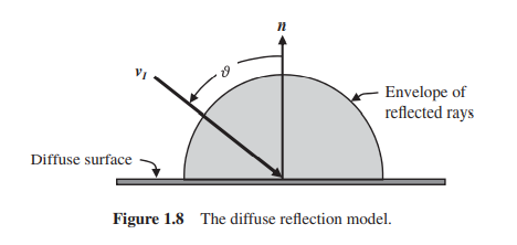
经验证实,来自表面的反射通常既不是漫反射也不是镜面反射。相反,在给定波长下,反射能量的分布取决于机械和化学制备
表面和入射方向。漫反射和镜面反射代表双向反射率的两个极端。这两个极端都可以接近,但在实践中很少能实现。已经提出了各种理论来预测通用表面的双向光谱反射和定向光谱发射和吸收。感兴趣的读者可以参考参考文献中的第 4 章。[1],其中更详细地探讨了该主题。然而,计量学仍然是获得准确捕捉真实表面的定向光谱行为的表面模型的唯一可靠途径。
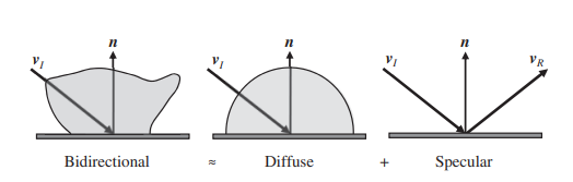
第 1 章介绍了一个简单的定向反射率双分量模型(图 1.9),其中建议定向反射模式在某种程度上可以近似为光谱和漫反射的适当加权组合。这种近似的不同版本必须应用于每个感兴趣的波长,对每个波长使用不同的权重因子。这种方法可能取得的任何成功在很大程度上归功于这样一个事实,即外壳内的辐射能分布由积分方程而不是微分方程控制。如图 4.1 所示,整合至少部分地“平均”了现实中的正负偏移。对该图的检查表明,即使
F1(X)是对局部行为的更详细和可能更准确的描述F2(X),但在可接受的近似值上,它可能是正确的,即
∫01F1(X)dX≅∫01F2(X)dX
统计代写|蒙特卡洛方法代写Monte Carlo method代考|Principles Underlying a Practical Bidirectional Reflection Model
有用的双向反射模型通常基于测量值,尽管它们经常受到理论的影响。正如我们在章节中学到的2.12和2.13,不导电(电介质)和导电(金属)表面的光学行为根本不同。一般来说,金属表面是强镜面反射器,而电介质表面往往是弱漫反射器。在这两种情况下,反射辐射的方向分布都受到表面的地形、化学状态和污染程度的强烈影响。除了某些光学组件(例如镜子、透镜和滤光片)之外,完全基于理论的双向光谱反射率模型不太可能准确地表示具有实际工程兴趣的表面的光学行为。因此,在需要高精度的情况下,
在本章中,我们首先展示了半经验方法对两种表面涂层的应用,这些涂层被设计为展示特定的−并且有些独特 – 光学行为。在第一个示例中,我们考虑了一种高吸收性商业涂层,其反射率的小部分高度定向到几乎是镜面的点,在第二个示例中,我们考虑了另一种高反射率但反射率几乎是漫射的商业涂层。这两种涂层都广泛用于需要金属和介电行为的不寻常组合的光学应用。然后,我们提出了一种完全通用的方法,适用于有全套实验数据的应用程序。
我们首先回顾第 2 章中的双向光谱反射率,ρλ′′=ρ(λ,ϑ一世,披一世,ϑr,披r)≡d一世λ,r(λ,ϑ一世,披一世,ϑr,披r)一世λ,一世(λ,ϑ一世,披一世)因ϑ一世dΩ一世 ≡乙RDF(λ,ϑ一世,披一世,ϑr,披r)

统计代写请认准statistics-lab™. statistics-lab™为您的留学生涯保驾护航。
金融工程代写
金融工程是使用数学技术来解决金融问题。金融工程使用计算机科学、统计学、经济学和应用数学领域的工具和知识来解决当前的金融问题,以及设计新的和创新的金融产品。
非参数统计代写
非参数统计指的是一种统计方法,其中不假设数据来自于由少数参数决定的规定模型;这种模型的例子包括正态分布模型和线性回归模型。
广义线性模型代考
广义线性模型(GLM)归属统计学领域,是一种应用灵活的线性回归模型。该模型允许因变量的偏差分布有除了正态分布之外的其它分布。
术语 广义线性模型(GLM)通常是指给定连续和/或分类预测因素的连续响应变量的常规线性回归模型。它包括多元线性回归,以及方差分析和方差分析(仅含固定效应)。
有限元方法代写
有限元方法(FEM)是一种流行的方法,用于数值解决工程和数学建模中出现的微分方程。典型的问题领域包括结构分析、传热、流体流动、质量运输和电磁势等传统领域。
有限元是一种通用的数值方法,用于解决两个或三个空间变量的偏微分方程(即一些边界值问题)。为了解决一个问题,有限元将一个大系统细分为更小、更简单的部分,称为有限元。这是通过在空间维度上的特定空间离散化来实现的,它是通过构建对象的网格来实现的:用于求解的数值域,它有有限数量的点。边界值问题的有限元方法表述最终导致一个代数方程组。该方法在域上对未知函数进行逼近。[1] 然后将模拟这些有限元的简单方程组合成一个更大的方程系统,以模拟整个问题。然后,有限元通过变化微积分使相关的误差函数最小化来逼近一个解决方案。
tatistics-lab作为专业的留学生服务机构,多年来已为美国、英国、加拿大、澳洲等留学热门地的学生提供专业的学术服务,包括但不限于Essay代写,Assignment代写,Dissertation代写,Report代写,小组作业代写,Proposal代写,Paper代写,Presentation代写,计算机作业代写,论文修改和润色,网课代做,exam代考等等。写作范围涵盖高中,本科,研究生等海外留学全阶段,辐射金融,经济学,会计学,审计学,管理学等全球99%专业科目。写作团队既有专业英语母语作者,也有海外名校硕博留学生,每位写作老师都拥有过硬的语言能力,专业的学科背景和学术写作经验。我们承诺100%原创,100%专业,100%准时,100%满意。
随机分析代写
随机微积分是数学的一个分支,对随机过程进行操作。它允许为随机过程的积分定义一个关于随机过程的一致的积分理论。这个领域是由日本数学家伊藤清在第二次世界大战期间创建并开始的。
时间序列分析代写
随机过程,是依赖于参数的一组随机变量的全体,参数通常是时间。 随机变量是随机现象的数量表现,其时间序列是一组按照时间发生先后顺序进行排列的数据点序列。通常一组时间序列的时间间隔为一恒定值(如1秒,5分钟,12小时,7天,1年),因此时间序列可以作为离散时间数据进行分析处理。研究时间序列数据的意义在于现实中,往往需要研究某个事物其随时间发展变化的规律。这就需要通过研究该事物过去发展的历史记录,以得到其自身发展的规律。
回归分析代写
多元回归分析渐进(Multiple Regression Analysis Asymptotics)属于计量经济学领域,主要是一种数学上的统计分析方法,可以分析复杂情况下各影响因素的数学关系,在自然科学、社会和经济学等多个领域内应用广泛。
MATLAB代写
MATLAB 是一种用于技术计算的高性能语言。它将计算、可视化和编程集成在一个易于使用的环境中,其中问题和解决方案以熟悉的数学符号表示。典型用途包括:数学和计算算法开发建模、仿真和原型制作数据分析、探索和可视化科学和工程图形应用程序开发,包括图形用户界面构建MATLAB 是一个交互式系统,其基本数据元素是一个不需要维度的数组。这使您可以解决许多技术计算问题,尤其是那些具有矩阵和向量公式的问题,而只需用 C 或 Fortran 等标量非交互式语言编写程序所需的时间的一小部分。MATLAB 名称代表矩阵实验室。MATLAB 最初的编写目的是提供对由 LINPACK 和 EISPACK 项目开发的矩阵软件的轻松访问,这两个项目共同代表了矩阵计算软件的最新技术。MATLAB 经过多年的发展,得到了许多用户的投入。在大学环境中,它是数学、工程和科学入门和高级课程的标准教学工具。在工业领域,MATLAB 是高效研究、开发和分析的首选工具。MATLAB 具有一系列称为工具箱的特定于应用程序的解决方案。对于大多数 MATLAB 用户来说非常重要,工具箱允许您学习和应用专业技术。工具箱是 MATLAB 函数(M 文件)的综合集合,可扩展 MATLAB 环境以解决特定类别的问题。可用工具箱的领域包括信号处理、控制系统、神经网络、模糊逻辑、小波、仿真等。