如果你也在 怎样代写贝叶斯分析Bayesian Analysis这个学科遇到相关的难题,请随时右上角联系我们的24/7代写客服。
贝叶斯分析,一种统计推断方法(以英国数学家托马斯-贝叶斯命名),允许人们将关于人口参数的先验信息与样本所含信息的证据相结合,以指导统计推断过程。
statistics-lab™ 为您的留学生涯保驾护航 在代写贝叶斯分析Bayesian Analysis方面已经树立了自己的口碑, 保证靠谱, 高质且原创的统计Statistics代写服务。我们的专家在代写贝叶斯分析Bayesian Analysis代写方面经验极为丰富,各种代写贝叶斯分析Bayesian Analysis相关的作业也就用不着说。
我们提供的贝叶斯分析Bayesian Analysis及其相关学科的代写,服务范围广, 其中包括但不限于:
- Statistical Inference 统计推断
- Statistical Computing 统计计算
- Advanced Probability Theory 高等概率论
- Advanced Mathematical Statistics 高等数理统计学
- (Generalized) Linear Models 广义线性模型
- Statistical Machine Learning 统计机器学习
- Longitudinal Data Analysis 纵向数据分析
- Foundations of Data Science 数据科学基础
统计代写|贝叶斯分析代写Bayesian Analysis代考|Credibility estimates
In actuarial studies, a credibility estimate is one which can be expressed as a weighted average of the form
$$
C=(1-k) A+k B \text {, }
$$
where:
$\begin{array}{ll}A & \text { is the subjective estimate (or the collateral data estimate) } \ B & \text { is the objective estimate (or the direct data estimate) } \ k \quad \text { is the credibility factor, a number that is between } 0 \text { and } 1 \ & \text { (inclusive) and represents the weight assigned to the } \ \text { objective estimate. }\end{array}$
A high value of $k$ implies $C \cong B$, representing a situation where the objective estimate is assigned ‘high credibility’. A primary aim of credibility theory is to determine an appropriate value or formula for $k$, as is done, for example, in the theory of the Bühlmann model (Bühlmann, 1967). Many Bayesian models lead to a point estimate which can be expressed as an intuitively appealing credibility estimate.
Earlier we showed that
$$
(\theta \mid y) \sim \operatorname{Beta}(\alpha+y, \beta+n-y),
$$
and hence that the posterior mean of $\theta$ is
$$
\hat{\theta}=E(\theta \mid y)=\frac{(\alpha+y)}{(\alpha+y)+(\beta+n-y)}=\frac{\alpha+y}{\alpha+\beta+n}
$$
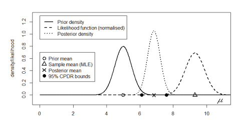
Observe that the prior mean of $\theta$ is $E \theta=\alpha /(\alpha+\beta)$, and the maximum likelihood estimate (MLE) of $\theta$ is $y / n$. This suggests that we write
$$
\begin{aligned}
\hat{\theta} &=\frac{\alpha}{\alpha+\beta+n}+\frac{y}{\alpha+\beta+n} \
&=\frac{\alpha}{\alpha+\beta+n}\left(\frac{\alpha+\beta}{\alpha}\right)\left(\frac{\alpha}{\alpha+\beta}\right)+\frac{n}{\alpha+\beta+n}\left(\frac{y}{n}\right) \
&=\frac{\alpha+\beta}{\alpha+\beta+n}\left(\frac{\alpha}{\alpha+\beta}\right)+\frac{n}{\alpha+\beta+n}\left(\frac{y}{n}\right)
\end{aligned}
$$
Thus $\hat{\theta}=(1-k) A+k B$
where: $\quad A=\frac{\alpha}{\alpha+\beta}, \quad B=\frac{y}{n}, \quad k=\frac{n}{\alpha+\beta+n}$.
We see that the posterior mean $\hat{\theta}$ is a credibility estimate in the form of a weighted average of the prior mean $A=E \theta=\alpha /(\alpha+\beta)$ and the MLE $B=y / n$, where the weight assigned to the MLE is the credibility factor given by $k=n /(n+\alpha+\beta)$. Observe that as $n$ increases, the credibility factor $k$ approaches 1 . This makes sense: if there is a lot of data then the prior should not have much influence on the estimation.
统计代写|贝叶斯分析代写Bayesian Analysis代考|Frequentist characteristics of Bayesian estimators
Consider a Bayesian model defined by a likelihood $f(y \mid \theta)$ and a prior $f(\theta)$, leading to the posterior
$$
f(\theta \mid y)=\frac{f(\theta) f(y \mid \theta)}{f(y)}
$$
Suppose that we choose to perform inference on $\theta$ by constructing a point estimate $\hat{\theta}$ (such as the posterior mean, mode or median) and a $(1-\alpha)$-level interval estimate $I=(L, U)$ (such as the CPDR or HPDR).
Then $\hat{\theta}, I, L$ and $U$ are functions of the data $y$ and may be written $\hat{\theta}(y)$, $I(y), L(y)$ and $U(y)$. Once these functions are defined, the estimates which they define stand on their own, so to speak, and may be studied from many different perspectives.
Naturally, the characteristics of these estimates may be seen in the context of the Bayesian framework in which they were constructed. More will be said on this below when we come to discuss Bayesian decision theory.
However, another important use of Bayesian estimates is as a proxy for classical estimates. We have already mentioned this in relation to the normal-normal model:
$$
\begin{aligned}
&\left(y_{1}, \ldots, y_{n} \mid \mu\right) \sim \text { iid } N\left(\mu, \sigma^{2}\right) \
&\mu \sim N\left(\mu_{0}, \sigma_{0}^{2}\right)
\end{aligned}
$$
where the use of a particular prior, namely the one specified by $\sigma_{0}=\infty$, led to the point estimate $\hat{\mu}=\hat{\mu}(y)=\bar{y}$ and the interval estimate
$$
I(y)=(L(y), U(y))=\left(\bar{y} \pm z_{\alpha / 2} \sigma / \sqrt{n}\right) .
$$
As we noted earlier, these estimates are exactly the same as the usual estimates used in the context of the corresponding classical model, $$
y_{1}, \ldots, y_{n} \sim i i d N\left(\mu, \sigma^{2}\right),
$$
where $\mu$ is an unknown constant and $\sigma^{2}$ is given.
统计代写|贝叶斯分析代写Bayesian Analysis代考|Mixture prior distributions
So far we have considered Bayesian models with priors that are limited in the types of prior information that they can represent. For example, the normal-normal model does not allow a prior for the normal mean which has two or more modes. If a non-normal class of prior is used to represent one’s complicated prior beliefs regarding the normal mean, then that prior will not be conjugate, and this will lead to difficulties down the track when making inferences based on the nonstandard posterior distribution.
Fortunately, this problem can be addressed in any Bayesian model for which a conjugate class of prior exists by specifying the prior as a mixture of members of that class.
Generally, a random variable $X$ with a mixture distribution has a density of the form
$$
f(x)=\sum_{m=1}^{M} c_{m} f_{m}(x),
$$
where each $f_{m}(x)$ is a proper density and the $c_{m}$ values are positive and sum to 1 .
If our prior beliefs regarding a parameter $\theta$ do not follow any single well-known distribution, those beliefs can in that case be conveniently approximated to any degree of precision by a suitable mixture prior distribution with a density having the form
$$
f(\theta)=\sum_{m=1}^{M} c_{m} f_{m}(\theta) .
$$
It can be shown (see Exercise $2.3$ below) that if each component prior $f_{m}(\theta)$ is conjugate then $f(\theta)$ is also conjugate. This means that $\theta$ ‘s posterior distribution is also a mixture with density of the form
$$
f(\theta \mid y)=\sum_{m=1}^{M} c_{m}^{\prime} f_{m}(\theta \mid y),
$$
where $f_{m}(\theta \mid y)$ is the posterior implied by the $m$ th prior $f_{m}(\theta)$ and is from the same family of distributions as that prior.
贝叶斯分析代考
统计代写|贝叶斯分析代写Bayesian Analysis代考|Credibility estimates
在精算研究中,可信度估计是一种可以表示为形式的加权平均值的估计
C=(1−ķ)一个+ķ乙,
在哪里:
一个 是主观估计(或抵押数据估计) 乙 是客观估计(或直接数据估计) ķ 是可信度因子,介于 0 和 1 (含)并表示分配给 客观估计。
高价值ķ暗示C≅乙,表示客观估计被赋予“高可信度”的情况。可信度理论的主要目的是确定一个适当的值或公式ķ,例如,在 Bühlmann 模型的理论中所做的 (Bühlmann, 1967)。许多贝叶斯模型导致点估计,可以表示为直观吸引人的可信度估计。
早些时候我们展示了
(θ∣是)∼贝塔(一个+是,b+n−是),
因此,后验均值θ是
θ^=和(θ∣是)=(一个+是)(一个+是)+(b+n−是)=一个+是一个+b+n
观察到先验均值θ是和θ=一个/(一个+b), 最大似然估计 (MLE)θ是是/n. 这表明我们写
θ^=一个一个+b+n+是一个+b+n =一个一个+b+n(一个+b一个)(一个一个+b)+n一个+b+n(是n) =一个+b一个+b+n(一个一个+b)+n一个+b+n(是n)
因此θ^=(1−ķ)一个+ķ乙
在哪里:一个=一个一个+b,乙=是n,ķ=n一个+b+n.
我们看到后验均值θ^是先前均值的加权平均形式的可信度估计一个=和θ=一个/(一个+b)和 MLE乙=是/n,其中分配给 MLE 的权重是由下式给出的可信度因子ķ=n/(n+一个+b). 观察到n增加,可信度因素ķ接近 1 . 这是有道理的:如果有很多数据,那么先验应该不会对估计产生太大影响。
统计代写|贝叶斯分析代写Bayesian Analysis代考|Frequentist characteristics of Bayesian estimators
考虑一个由可能性定义的贝叶斯模型F(是∣θ)和之前的F(θ), 导致后
F(θ∣是)=F(θ)F(是∣θ)F(是)
假设我们选择对θ通过构建点估计θ^(例如后验均值、众数或中位数)和(1−一个)水平区间估计我=(大号,在)(例如 CPDR 或 HPDR)。
然后θ^,我,大号和在是数据的函数是并且可以写成θ^(是), 我(是),大号(是)和在(是). 一旦定义了这些函数,它们定义的估计就可以说是独立存在的,并且可以从许多不同的角度进行研究。
自然地,这些估计的特征可以在构建它们的贝叶斯框架的背景下看到。当我们讨论贝叶斯决策理论时,下面将对此进行更多说明。
然而,贝叶斯估计的另一个重要用途是作为经典估计的代理。我们已经在法线-法线模型中提到了这一点:
(是1,…,是n∣μ)∼ 独立同居 ñ(μ,σ2) μ∼ñ(μ0,σ02)
其中使用特定的先验,即由σ0=∞,导致点估计μ^=μ^(是)=是¯和区间估计
我(是)=(大号(是),在(是))=(是¯±和一个/2σ/n).
正如我们之前提到的,这些估计与在相应经典模型的上下文中使用的通常估计完全相同,
是1,…,是n∼一世一世dñ(μ,σ2),
在哪里μ是一个未知常数并且σ2给出。
统计代写|贝叶斯分析代写Bayesian Analysis代考|Mixture prior distributions
到目前为止,我们已经考虑了具有先验的贝叶斯模型,这些模型在它们可以表示的先验信息类型方面受到限制。例如,正态-正态模型不允许具有两个或多个模态的正态平均值的先验。如果使用非正态先验类别来表示一个人对正态均值的复杂先验信念,则该先验将不是共轭的,这将导致在基于非标准后验分布进行推断时遇到困难。
幸运的是,这个问题可以在任何存在共轭先验类的贝叶斯模型中解决,方法是将先验指定为该类成员的混合。
一般来说,随机变量X具有混合分布的密度为
F(X)=∑米=1米C米F米(X),
其中每个F米(X)是一个适当的密度和C米值为正且总和为 1 。
如果我们对参数的先前信念θ不遵循任何单一的众所周知的分布,在那种情况下,这些信念可以方便地通过适当的混合先验分布以任何精度近似,其密度具有以下形式
F(θ)=∑米=1米C米F米(θ).
它可以显示(见练习2.3下面),如果每个组件之前F米(θ)那么是共轭的F(θ)也是共轭的。这意味着θ的后验分布也是与密度的混合形式
F(θ∣是)=∑米=1米C米′F米(θ∣是),
在哪里F米(θ∣是)是由米先验F米(θ)并且来自与先前相同的分布系列。

统计代写请认准statistics-lab™. statistics-lab™为您的留学生涯保驾护航。
金融工程代写
金融工程是使用数学技术来解决金融问题。金融工程使用计算机科学、统计学、经济学和应用数学领域的工具和知识来解决当前的金融问题,以及设计新的和创新的金融产品。
非参数统计代写
非参数统计指的是一种统计方法,其中不假设数据来自于由少数参数决定的规定模型;这种模型的例子包括正态分布模型和线性回归模型。
广义线性模型代考
广义线性模型(GLM)归属统计学领域,是一种应用灵活的线性回归模型。该模型允许因变量的偏差分布有除了正态分布之外的其它分布。
术语 广义线性模型(GLM)通常是指给定连续和/或分类预测因素的连续响应变量的常规线性回归模型。它包括多元线性回归,以及方差分析和方差分析(仅含固定效应)。
有限元方法代写
有限元方法(FEM)是一种流行的方法,用于数值解决工程和数学建模中出现的微分方程。典型的问题领域包括结构分析、传热、流体流动、质量运输和电磁势等传统领域。
有限元是一种通用的数值方法,用于解决两个或三个空间变量的偏微分方程(即一些边界值问题)。为了解决一个问题,有限元将一个大系统细分为更小、更简单的部分,称为有限元。这是通过在空间维度上的特定空间离散化来实现的,它是通过构建对象的网格来实现的:用于求解的数值域,它有有限数量的点。边界值问题的有限元方法表述最终导致一个代数方程组。该方法在域上对未知函数进行逼近。[1] 然后将模拟这些有限元的简单方程组合成一个更大的方程系统,以模拟整个问题。然后,有限元通过变化微积分使相关的误差函数最小化来逼近一个解决方案。
tatistics-lab作为专业的留学生服务机构,多年来已为美国、英国、加拿大、澳洲等留学热门地的学生提供专业的学术服务,包括但不限于Essay代写,Assignment代写,Dissertation代写,Report代写,小组作业代写,Proposal代写,Paper代写,Presentation代写,计算机作业代写,论文修改和润色,网课代做,exam代考等等。写作范围涵盖高中,本科,研究生等海外留学全阶段,辐射金融,经济学,会计学,审计学,管理学等全球99%专业科目。写作团队既有专业英语母语作者,也有海外名校硕博留学生,每位写作老师都拥有过硬的语言能力,专业的学科背景和学术写作经验。我们承诺100%原创,100%专业,100%准时,100%满意。
随机分析代写
随机微积分是数学的一个分支,对随机过程进行操作。它允许为随机过程的积分定义一个关于随机过程的一致的积分理论。这个领域是由日本数学家伊藤清在第二次世界大战期间创建并开始的。
时间序列分析代写
随机过程,是依赖于参数的一组随机变量的全体,参数通常是时间。 随机变量是随机现象的数量表现,其时间序列是一组按照时间发生先后顺序进行排列的数据点序列。通常一组时间序列的时间间隔为一恒定值(如1秒,5分钟,12小时,7天,1年),因此时间序列可以作为离散时间数据进行分析处理。研究时间序列数据的意义在于现实中,往往需要研究某个事物其随时间发展变化的规律。这就需要通过研究该事物过去发展的历史记录,以得到其自身发展的规律。
回归分析代写
多元回归分析渐进(Multiple Regression Analysis Asymptotics)属于计量经济学领域,主要是一种数学上的统计分析方法,可以分析复杂情况下各影响因素的数学关系,在自然科学、社会和经济学等多个领域内应用广泛。
MATLAB代写
MATLAB 是一种用于技术计算的高性能语言。它将计算、可视化和编程集成在一个易于使用的环境中,其中问题和解决方案以熟悉的数学符号表示。典型用途包括:数学和计算算法开发建模、仿真和原型制作数据分析、探索和可视化科学和工程图形应用程序开发,包括图形用户界面构建MATLAB 是一个交互式系统,其基本数据元素是一个不需要维度的数组。这使您可以解决许多技术计算问题,尤其是那些具有矩阵和向量公式的问题,而只需用 C 或 Fortran 等标量非交互式语言编写程序所需的时间的一小部分。MATLAB 名称代表矩阵实验室。MATLAB 最初的编写目的是提供对由 LINPACK 和 EISPACK 项目开发的矩阵软件的轻松访问,这两个项目共同代表了矩阵计算软件的最新技术。MATLAB 经过多年的发展,得到了许多用户的投入。在大学环境中,它是数学、工程和科学入门和高级课程的标准教学工具。在工业领域,MATLAB 是高效研究、开发和分析的首选工具。MATLAB 具有一系列称为工具箱的特定于应用程序的解决方案。对于大多数 MATLAB 用户来说非常重要,工具箱允许您学习和应用专业技术。工具箱是 MATLAB 函数(M 文件)的综合集合,可扩展 MATLAB 环境以解决特定类别的问题。可用工具箱的领域包括信号处理、控制系统、神经网络、模糊逻辑、小波、仿真等。