如果你也在 怎样代写贝叶斯统计这个学科遇到相关的难题,请随时右上角联系我们的24/7代写客服。
贝叶斯统计学是一个使用概率的数学语言来描述认识论的不确定性的系统。在 “贝叶斯范式 “中,对自然状态的相信程度是明确的;这些程度是非负的,而对所有自然状态的总相信是固定的。
statistics-lab™ 为您的留学生涯保驾护航 在代写贝叶斯统计方面已经树立了自己的口碑, 保证靠谱, 高质且原创的统计Statistics代写服务。我们的专家在代写贝叶斯统计代写方面经验极为丰富,各种代写贝叶斯统计相关的作业也就用不着说。
我们提供的贝叶斯统计及其相关学科的代写,服务范围广, 其中包括但不限于:
- Statistical Inference 统计推断
- Statistical Computing 统计计算
- Advanced Probability Theory 高等概率论
- Advanced Mathematical Statistics 高等数理统计学
- (Generalized) Linear Models 广义线性模型
- Statistical Machine Learning 统计机器学习
- Longitudinal Data Analysis 纵向数据分析
- Foundations of Data Science 数据科学基础
统计代写|贝叶斯统计代写beyesian statistics代考|Non-spatial graphical exploration
Recall the air pollution data set nysptime introduced in Section $1.3 .1$ which contains the daily maximum ozone concentration values at the 28 sites shown in Figure $1.1$ in the state of New York for the 62 days in July and August 2006. From this data set we have created a spatial data set, named nyspatial, which contains the average air pollution and the average values of the three covariates at the 28 sites. Figure $3.1$ provides a histogram for the response, average daily ozone concentration levels, at the 28 monitoring sites. The plot does not show a symmetric bell-shaped histogram but it does admit the possibility of a unimodal distribution for the response. The $R$ command used to draw the plot is given below:
The geom_histogram command has been invoked with a bin width argument of $4.5$. The shape of the histogram will change if a different bin width is supplied. As is well known, a lower value will provide a lesser degree of smoothing while a higher value will increase more smoothing by collapsing the number of classes. It is also possible to adopt a different scale, e.g. square root or logarithm, but we have not done so here to illustrate modeling on the original scale of the data. We shall explore different scales for the spatio-temporal version of this data set.
Figure $3.2$ provides a pair-wise scatter plot of the response against the three explanatory covariates: maximum temperature, wind speed and relative humidity. The diagonal panels in this plot provides kernel density estimates of the variables. This plot reveals that wind speed correlates the most with ozone levels at this aggregated average level. As is well known, see e.g. Sahu and Bakar (2012a), the maximum temperature also positively correlates with the ozone levels. Relative humidity is seen to have the least amount of correlation with ozone levels. This plot has been obtained using the commands.
统计代写|贝叶斯统计代写beyesian statistics代考|Exploring spatio-temporal point reference data
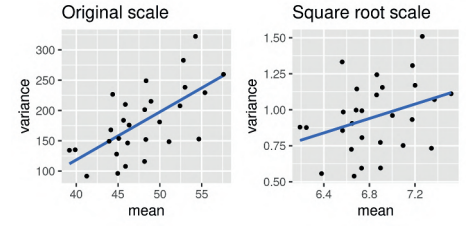
This section illustrates EDA methods with the nysptime data set in bmstdr. To decide the modeling scale Figure $3.5$ plots the mean against variance for each site on the original scale and also on the square root scale for the response. A stronger linear mean-variance relationship with a larger value of the slope for the superimposed regression line is observed on the original scale making this less suitable for modeling purposes. This is because in linear statistical modeling we often model the mean as a function of the available covariates and assume equal variance (homoscedasticity) for the residual differences between the observed and modeled values. A word of caution here is that the right panel does not show a complete lack of mean-variance relationship. However, we still prefer to model on the square root scale to stabilize the variance and in this case the predictions we make in Chapter 7 for ozone concentration values do not become negative.
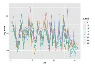
Temporal variations are illustrated in Figures $3.6$ for all 28 sites and in Figure $3.8$ for the 8 sites which have been used for model validation purposes in Chapters 6 and 7. Figure $3.7$ shows variations of ozone concentration values for the 28 monitoring sites. Suspected outliers, data values which are at a distance beyond $1.5$ times the inter quartile range from the whiskers, are plotted as red stars. Such high values of ground level ozone pollution are especially harmful to humans.
统计代写|贝叶斯统计代写beyesian statistics代考|Exploring areal Covid-19 case and death data
This section explores the Covid-19 mortality data introduced in Section 1.4.1. The bmstdr data frame engtotals contains aggregated number of deaths along with other relevant information for analyzing and modeling this data set. The data frame object engdeaths contains the death numbers by the 20 weeks from March 13 to July 31,2020 . These two data sets will be used to illustrate spatial and spatio-temporal modeling for areal data in Chapter 10 .
Typical such areal data are represented by a choropleth map which uses shades of color or grey scale to classify values into a few broad classes, like a histogram. Two choropleth maps have been provided in Figure $1.9$.
For the engtotals data set the minimum and maximum number of deaths were 4 and 1223 respectively for the City of London (a very small borough within greater London with population 9721) and Birmingham with population $1,141,816$ in 2019 . However, the minimum and maximum death rates per 100,000 were $10.79$ and $172.51$ respectively for Hastings (in the South East) and Hertsmere (near Watford in greater London) respectively.
Calculation of the Moran’s I for number and rate of deaths is performed by using the moran .me function in the library spdep. This function requires the spatial adjacency matrix in a list format, which is obtained by the poly2nb and nb2listw functions in the spdep library. The Moran’s I statistics for the raw observed death numbers and the rate are found to be $0.34$ and $0.45$ respectively both with a p-value smaller than $0.001$ for the null hypothesis of no spatial autocorrelation. The permutation tests in statistics randomly permute the observed data and then calculates the relevant statistics for a number of replications. These replicate values of the statistics are used to approximate the null distribution of the statistics against which the observed value of the statistics for the observed data is compared and an approximate $\mathrm{p}$-value is found. The tests with Geary’s $\mathrm{C}$ statistics gave a $\mathrm{p}$-value of less than $0.001$ for the death rate per 100,000 but the p-value was higher, $0.025$, for the un-adjusted observed Covid death numbers. Thus, the higher degree of spatial variation in the death rates has been successfully detected by the Geary’s statistics. The code lines to obtain these results are given below.
贝叶斯统计代写
统计代写|贝叶斯统计代写beyesian statistics代考|Non-spatial graphical exploration
回想一下第 1 节介绍的空气污染数据集 nysptime1.3.1其中包含图 1 所示 28 个站点的每日最大臭氧浓度值1.12006 年 7 月和 8 月在纽约州的 62 天。根据该数据集,我们创建了一个名为 nyspatial 的空间数据集,其中包含 28 个站点的平均空气污染和三个协变量的平均值。数字3.1提供了 28 个监测点的响应直方图,即平均每日臭氧浓度水平。该图未显示对称的钟形直方图,但确实承认响应存在单峰分布的可能性。这R用于绘制绘图的命令如下:
已使用 bin 宽度参数调用 geom_histogram 命令4.5. 如果提供不同的 bin 宽度,直方图的形状将发生变化。众所周知,较低的值将提供较小程度的平滑,而较高的值将通过折叠类的数量来增加更多的平滑度。也可以采用不同的尺度,例如平方根或对数,但我们在这里没有这样做来说明对数据原始尺度的建模。我们将探索该数据集时空版本的不同尺度。
数字3.2提供了对三个解释性协变量的响应的成对散点图:最高温度、风速和相对湿度。该图中的对角线面板提供了变量的核密度估计。该图显示,风速与此聚合平均水平的臭氧水平最相关。众所周知,参见例如 Sahu 和 Bakar (2012a),最高温度也与臭氧水平正相关。相对湿度被认为与臭氧水平的相关性最小。该图是使用命令获得的。
统计代写|贝叶斯统计代写beyesian statistics代考|Exploring spatio-temporal point reference data
本节说明使用 bmstdr 中的 nysptime 数据集的 EDA 方法。决定造型比例图3.5在原始尺度以及响应的平方根尺度上绘制每个站点的均值与方差。在原始尺度上观察到叠加回归线的斜率值越大,线性均值-方差关系越强,因此不太适合建模目的。这是因为在线性统计建模中,我们经常将平均值建模为可用协变量的函数,并假设观测值和建模值之间的残差差异相等(同方差性)。这里需要注意的是,右侧面板并未显示完全缺乏均值-方差关系。但是,我们仍然更喜欢在平方根尺度上建模以稳定方差,在这种情况下,我们在第 7 章中对臭氧浓度值所做的预测不会变为负值。
时间变化如图所示3.6对于所有 28 个站点,在图3.8用于第 6 章和第 7 章中用于模型验证目的的 8 个站点。图3.7显示了 28 个监测点的臭氧浓度值的变化。可疑的异常值,超出距离的数据值1.5将晶须的四分位间距乘以红色星形。如此高的地面臭氧污染值对人类尤其有害。
统计代写|贝叶斯统计代写beyesian statistics代考|Exploring areal Covid-19 case and death data
本节探讨第 1.4.1 节中介绍的 Covid-19 死亡率数据。bmstdr 数据框 engtotals 包含汇总的死亡人数以及用于分析和建模此数据集的其他相关信息。数据框对象 engdeaths 包含从 2020 年 3 月 13 日到 7 月 31 日这 20 周的死亡人数。这两个数据集将在第 10 章中用于说明区域数据的空间和时空建模。
典型的此类区域数据由等值线图表示,该图使用颜色或灰度的阴影将值分类为几个大类,如直方图。图中提供了两个等值线图1.9.
对于 enttotals 数据集,伦敦金融城(大伦敦内的一个非常小的行政区,人口 9721)和伯明翰的人口最少和最大死亡人数分别为 4 和 12231,141,816在 2019 年。然而,每 100,000 人的最低和最高死亡率分别为10.79和172.51分别是黑斯廷斯(东南部)和赫茨米尔(大伦敦沃特福德附近)。
使用库 spdep 中的 moran .me 函数计算死亡人数和死亡率的 Moran’s I。该函数需要列表格式的空间邻接矩阵,由spdep库中的poly2nb和nb2listw函数获取。发现原始观察到的死亡人数和死亡率的 Moran’s I 统计数据为0.34和0.45分别具有小于的 p 值0.001对于没有空间自相关的原假设。统计中的排列测试随机排列观察到的数据,然后计算多次重复的相关统计量。这些统计量的重复值用于近似统计量的零分布,观察数据的统计量的观察值与之进行比较,以及一个近似值p- 找到值。与 Geary 的测试C统计给出了一个p-值小于0.001对于每 100,000 人的死亡率,但 p 值更高,0.025,对于未调整的观察到的 Covid 死亡人数。因此,Geary 的统计数据已经成功地检测到死亡率的更高程度的空间变化。下面给出了获得这些结果的代码行。

统计代写请认准statistics-lab™. statistics-lab™为您的留学生涯保驾护航。
金融工程代写
金融工程是使用数学技术来解决金融问题。金融工程使用计算机科学、统计学、经济学和应用数学领域的工具和知识来解决当前的金融问题,以及设计新的和创新的金融产品。
非参数统计代写
非参数统计指的是一种统计方法,其中不假设数据来自于由少数参数决定的规定模型;这种模型的例子包括正态分布模型和线性回归模型。
广义线性模型代考
广义线性模型(GLM)归属统计学领域,是一种应用灵活的线性回归模型。该模型允许因变量的偏差分布有除了正态分布之外的其它分布。
术语 广义线性模型(GLM)通常是指给定连续和/或分类预测因素的连续响应变量的常规线性回归模型。它包括多元线性回归,以及方差分析和方差分析(仅含固定效应)。
有限元方法代写
有限元方法(FEM)是一种流行的方法,用于数值解决工程和数学建模中出现的微分方程。典型的问题领域包括结构分析、传热、流体流动、质量运输和电磁势等传统领域。
有限元是一种通用的数值方法,用于解决两个或三个空间变量的偏微分方程(即一些边界值问题)。为了解决一个问题,有限元将一个大系统细分为更小、更简单的部分,称为有限元。这是通过在空间维度上的特定空间离散化来实现的,它是通过构建对象的网格来实现的:用于求解的数值域,它有有限数量的点。边界值问题的有限元方法表述最终导致一个代数方程组。该方法在域上对未知函数进行逼近。[1] 然后将模拟这些有限元的简单方程组合成一个更大的方程系统,以模拟整个问题。然后,有限元通过变化微积分使相关的误差函数最小化来逼近一个解决方案。
tatistics-lab作为专业的留学生服务机构,多年来已为美国、英国、加拿大、澳洲等留学热门地的学生提供专业的学术服务,包括但不限于Essay代写,Assignment代写,Dissertation代写,Report代写,小组作业代写,Proposal代写,Paper代写,Presentation代写,计算机作业代写,论文修改和润色,网课代做,exam代考等等。写作范围涵盖高中,本科,研究生等海外留学全阶段,辐射金融,经济学,会计学,审计学,管理学等全球99%专业科目。写作团队既有专业英语母语作者,也有海外名校硕博留学生,每位写作老师都拥有过硬的语言能力,专业的学科背景和学术写作经验。我们承诺100%原创,100%专业,100%准时,100%满意。
随机分析代写
随机微积分是数学的一个分支,对随机过程进行操作。它允许为随机过程的积分定义一个关于随机过程的一致的积分理论。这个领域是由日本数学家伊藤清在第二次世界大战期间创建并开始的。
时间序列分析代写
随机过程,是依赖于参数的一组随机变量的全体,参数通常是时间。 随机变量是随机现象的数量表现,其时间序列是一组按照时间发生先后顺序进行排列的数据点序列。通常一组时间序列的时间间隔为一恒定值(如1秒,5分钟,12小时,7天,1年),因此时间序列可以作为离散时间数据进行分析处理。研究时间序列数据的意义在于现实中,往往需要研究某个事物其随时间发展变化的规律。这就需要通过研究该事物过去发展的历史记录,以得到其自身发展的规律。
回归分析代写
多元回归分析渐进(Multiple Regression Analysis Asymptotics)属于计量经济学领域,主要是一种数学上的统计分析方法,可以分析复杂情况下各影响因素的数学关系,在自然科学、社会和经济学等多个领域内应用广泛。
MATLAB代写
MATLAB 是一种用于技术计算的高性能语言。它将计算、可视化和编程集成在一个易于使用的环境中,其中问题和解决方案以熟悉的数学符号表示。典型用途包括:数学和计算算法开发建模、仿真和原型制作数据分析、探索和可视化科学和工程图形应用程序开发,包括图形用户界面构建MATLAB 是一个交互式系统,其基本数据元素是一个不需要维度的数组。这使您可以解决许多技术计算问题,尤其是那些具有矩阵和向量公式的问题,而只需用 C 或 Fortran 等标量非交互式语言编写程序所需的时间的一小部分。MATLAB 名称代表矩阵实验室。MATLAB 最初的编写目的是提供对由 LINPACK 和 EISPACK 项目开发的矩阵软件的轻松访问,这两个项目共同代表了矩阵计算软件的最新技术。MATLAB 经过多年的发展,得到了许多用户的投入。在大学环境中,它是数学、工程和科学入门和高级课程的标准教学工具。在工业领域,MATLAB 是高效研究、开发和分析的首选工具。MATLAB 具有一系列称为工具箱的特定于应用程序的解决方案。对于大多数 MATLAB 用户来说非常重要,工具箱允许您学习和应用专业技术。工具箱是 MATLAB 函数(M 文件)的综合集合,可扩展 MATLAB 环境以解决特定类别的问题。可用工具箱的领域包括信号处理、控制系统、神经网络、模糊逻辑、小波、仿真等。