如果你也在 怎样代写贝叶斯网络Bayesian network这个学科遇到相关的难题,请随时右上角联系我们的24/7代写客服。
贝叶斯网络(BN)是一种表示不确定领域知识的概率图形模型,其中每个节点对应一个随机变量,每条边代表相应随机变量的条件概率。
statistics-lab™ 为您的留学生涯保驾护航 在代写贝叶斯网络Bayesian network方面已经树立了自己的口碑, 保证靠谱, 高质且原创的统计Statistics代写服务。我们的专家在代写贝叶斯网络Bayesian network代写方面经验极为丰富,各种代写贝叶斯网络Bayesian network相关的作业也就用不着说。
我们提供的贝叶斯网络Bayesian network及其相关学科的代写,服务范围广, 其中包括但不限于:
- Statistical Inference 统计推断
- Statistical Computing 统计计算
- Advanced Probability Theory 高等概率论
- Advanced Mathematical Statistics 高等数理统计学
- (Generalized) Linear Models 广义线性模型
- Statistical Machine Learning 统计机器学习
- Longitudinal Data Analysis 纵向数据分析
- Foundations of Data Science 数据科学基础
统计代写|贝叶斯网络代写Bayesian network代考|B N R C-Based Prediction
Once all the tuned inferred values are produced, these are further processed to finally generate the predicted value of the variable. Among all the tuned inferred values of the prediction variable, the predicted value becomes the one which is associated with the highest probability estimates $P\left({ }^{*}\right)$ during inference generation. Therefore, if pre $d_{V_{j}}$ is the predicted value of the variable $V_{j}$, then pred $V_{V_{j}}=$ tuned_infer $_{V_{j}}^{(t+1)}$ such that $P\left(\operatorname{infer}{V} \mid e\right)=\max \left{P\left(V{j} \mid e\right)\right}$, where $e$ indicates the given combination of values for the set of evidence variables. Now, since the overall analysis is performed considering discretized value of the variables, the predicted value pred ${ }{V j}$ may also be obtained in the form of range of values $\left[L B{j}, U B_{j}\right]$. In order to get a single value for the prediction variable, the mid value of the range may be considered. Therefore, finally, pre $_{V_{j}}=\left(L B_{j}+U B_{j}\right) / 2$.
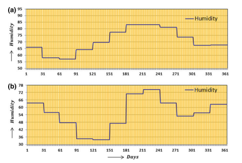
In the following part of the chapter, we attempt to present two separate case studies to validate the effectiveness of BNRC model in the context of spatial time series prediction under paucity of domain variables.
统计代写|贝叶斯网络代写Bayesian network代考|Experimental Setup
The architecture of the BNRC-based prediction system corresponding to the present case study is depicted in Fig. 3.8. The evaluation of the model is carried out in comparison with a number of benchmark time series prediction techniques, namely Automated Auto-regressive Integrated Moving Average (A-ARIMA), Vector Auto-regressive Moving Average (VARMA), Generalized Auto-regressive Heteroskedasticity (GARCH) model, neural network with feed forward back propagation (FFBP) [10], Recurrent Neural Network (RNN), Non-linear Auto-Regressive Neural Network (NARNET), Support Vector Machine (SVM), and the state-of-the-art space-time model based on
统计代写|贝叶斯网络代写Bayesian network代考|Results
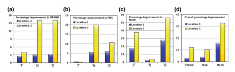
The performance of the BNRC and the other prediction techniques are measured in terms of four statistical measures, namely NRMSD, MAE, MAPE and $R^{2}$. The detailed mathematical formulations for these metrics are given below. In each case, $O_{\max }$ is the maximum observed (actual) value of the prediction variable, $O_{\min }$ is the minimum observed value of the prediction variable, $V_{o_{\mathrm{r}}}$ is the actual value corresponding to the $i$-th observation of the variable, $V_{p i}$ is the predicted value corresponding to the $i$-th observation of the variable, $\bar{V}{o}$ is the mean of observed/actual values of the prediction variable, $\overline{V{p}}$ is the mean of predicted values of the variable, and $N$ is the total number of observations.: The performance of the BNRC and the other prediction techniques are measured in terms of four statistical measures, namely NRMSD, MAE, MAPE and $R^{2}$. The detailed mathematical formulations for these metrics are given below. In each case, $O_{\max }$ is the maximum observed (actual) value of the prediction variable, $O_{\min }$ is the minimum observed value of the prediction variable, $V_{o_{\mathrm{r}}}$ is the actual value corresponding to the $i$-th observation of the variable, $V_{p i}$ is the predicted value corresponding to the $i$-th observation of the variable, $\bar{V}{o}$ is the mean of observed/actual values of the prediction variable, $\overline{V{p}}$ is the mean of predicted values of the variable, and $N$ is the total number of observations.:
$$
N R M S D=\frac{1}{\left(O_{\max }-O_{\min }\right)} \sqrt{\frac{1}{N} \sum_{i=1}^{N}\left(V_{o_{i}}-V_{p_{i}}\right)^{2}}
$$
NRMSD is also called Normalized Root Mean Square Error (NRMSE), and is often expressed in percentage ( $\%$ ). The best-fit between observed (actual) and predicted value under ideal conditions yields NRMSD $=0$.
$$
R^{2}=\frac{\left[\sum_{i=1}^{N}\left(V_{o_{i}}-\overline{V_{o}}\right)\left(V_{p_{i}}-\overline{V_{p}}\right)\right]^{2}}{\sum_{i=1}^{N}\left(V_{o_{i}}-\overline{V_{o}}\right)^{2} \cdot \sum_{i=1}^{N}\left(V_{p_{i}}-\overline{V_{p}}\right)^{2}}
$$
An $R^{2}$ value of 1 indicates a perfect fit between the observed and predicted value.
$$
M A E=\frac{1}{N} \sum_{i=1}^{N}\left|V_{o_{i}}-V_{p_{i}}\right|
$$
The best-fit between observed and predicted value under ideal conditions yields MAE $=0$.
$$
M A P E=\frac{\left|\overline{V_{o}}-\overline{V_{p}}\right|}{\left|\overline{V_{o}}\right|} \times 100
$$
The best-fit between observed (actual) and predicted value yields MAPE $=0$.
The comparative results of predicting Temperature $(\mathcal{T})$, Humidity $(\mathcal{H})$, and Precipitation rate $(\mathcal{R})$ are summarized in the Table $3.5$, Table $3.6$, and Table $3.7$, respectively.
贝叶斯网络代考
统计代写|贝叶斯网络代写Bayesian network代考|B N R C-Based Prediction
一旦产生了所有调整后的推断值,这些推断值将被进一步处理以最终生成变量的预测值。在预测变量的所有调整推断值中,预测值成为与最高概率估计相关联的值磷(∗)在推理生成期间。因此,如果预d在j是变量的预测值在j, 然后预在在j=tune_infer在j(吨+1)这样P\left(\operatorname{infer}{V} \mid e\right)=\max \left{P\left(V{j} \mid e\right)\right}P\left(\operatorname{infer}{V} \mid e\right)=\max \left{P\left(V{j} \mid e\right)\right}, 在哪里和表示一组证据变量的给定值组合。现在,由于整体分析是考虑变量的离散值进行的,因此预测值 pred在j也可以取值范围的形式[大号乙j,在乙j]. 为了获得预测变量的单个值,可以考虑范围的中间值。因此,最后,预在j=(大号乙j+在乙j)/2.
在本章的以下部分,我们尝试提出两个独立的案例研究,以验证 BNRC 模型在缺乏域变量的空间时间序列预测背景下的有效性。
统计代写|贝叶斯网络代写Bayesian network代考|Experimental Setup
对应于本案例研究的基于 BNRC 的预测系统的架构如图 3.8 所示。模型的评估是与许多基准时间序列预测技术进行比较的,即自动自回归综合移动平均线(A-ARIMA)、向量自回归移动平均线(VARMA)、广义自回归异方差( GARCH) 模型、具有前馈反向传播 (FFBP) [10] 的神经网络、循环神经网络 (RNN)、非线性自回归神经网络 (NARNET)、支持向量机 (SVM) 和状态最先进的时空模型
统计代写|贝叶斯网络代写Bayesian network代考|Results
BNRC 和其他预测技术的性能是根据四个统计指标来衡量的,即 NRMSD、MAE、MAPE 和R2. 下面给出了这些指标的详细数学公式。在每种情况下,○最大限度是预测变量的最大观察(实际)值,○分钟是预测变量的最小观测值,在○r是对应的实际值一世-对变量的第一次观察,在p一世是对应的预测值一世-对变量的第一次观察,在¯○是预测变量的观察值/实际值的平均值,在p¯是变量预测值的平均值,并且ñ是观察的总数。:BNRC 和其他预测技术的性能是根据四个统计指标来衡量的,即 NRMSD、MAE、MAPE 和R2. 下面给出了这些指标的详细数学公式。在每种情况下,○最大限度是预测变量的最大观察(实际)值,○分钟是预测变量的最小观测值,在○r是对应的实际值一世-对变量的第一次观察,在p一世是对应的预测值一世-对变量的第一次观察,在¯○是预测变量的观察值/实际值的平均值,在p¯是变量预测值的平均值,并且ñ是观察的总数。:
ñR米小号D=1(○最大限度−○分钟)1ñ∑一世=1ñ(在○一世−在p一世)2
NRMSD 也称为归一化均方根误差 (NRMSE),通常以百分比 (%)。理想条件下观察值(实际值)和预测值之间的最佳拟合产生 NRMSD=0.
R2=[∑一世=1ñ(在○一世−在○¯)(在p一世−在p¯)]2∑一世=1ñ(在○一世−在○¯)2⋅∑一世=1ñ(在p一世−在p¯)2
一个R2值 1 表示观察值和预测值之间的完美拟合。
米一个和=1ñ∑一世=1ñ|在○一世−在p一世|
理想条件下观测值和预测值之间的最佳拟合产生 MAE=0.
米一个磷和=|在○¯−在p¯||在○¯|×100
观察值(实际值)和预测值之间的最佳拟合产生 MAPE=0.
预测温度的比较结果(吨), 湿度(H), 和降水率(R)汇总于表中3.5, 桌子3.6, 和表3.7, 分别。

统计代写请认准statistics-lab™. statistics-lab™为您的留学生涯保驾护航。
金融工程代写
金融工程是使用数学技术来解决金融问题。金融工程使用计算机科学、统计学、经济学和应用数学领域的工具和知识来解决当前的金融问题,以及设计新的和创新的金融产品。
非参数统计代写
非参数统计指的是一种统计方法,其中不假设数据来自于由少数参数决定的规定模型;这种模型的例子包括正态分布模型和线性回归模型。
广义线性模型代考
广义线性模型(GLM)归属统计学领域,是一种应用灵活的线性回归模型。该模型允许因变量的偏差分布有除了正态分布之外的其它分布。
术语 广义线性模型(GLM)通常是指给定连续和/或分类预测因素的连续响应变量的常规线性回归模型。它包括多元线性回归,以及方差分析和方差分析(仅含固定效应)。
有限元方法代写
有限元方法(FEM)是一种流行的方法,用于数值解决工程和数学建模中出现的微分方程。典型的问题领域包括结构分析、传热、流体流动、质量运输和电磁势等传统领域。
有限元是一种通用的数值方法,用于解决两个或三个空间变量的偏微分方程(即一些边界值问题)。为了解决一个问题,有限元将一个大系统细分为更小、更简单的部分,称为有限元。这是通过在空间维度上的特定空间离散化来实现的,它是通过构建对象的网格来实现的:用于求解的数值域,它有有限数量的点。边界值问题的有限元方法表述最终导致一个代数方程组。该方法在域上对未知函数进行逼近。[1] 然后将模拟这些有限元的简单方程组合成一个更大的方程系统,以模拟整个问题。然后,有限元通过变化微积分使相关的误差函数最小化来逼近一个解决方案。
tatistics-lab作为专业的留学生服务机构,多年来已为美国、英国、加拿大、澳洲等留学热门地的学生提供专业的学术服务,包括但不限于Essay代写,Assignment代写,Dissertation代写,Report代写,小组作业代写,Proposal代写,Paper代写,Presentation代写,计算机作业代写,论文修改和润色,网课代做,exam代考等等。写作范围涵盖高中,本科,研究生等海外留学全阶段,辐射金融,经济学,会计学,审计学,管理学等全球99%专业科目。写作团队既有专业英语母语作者,也有海外名校硕博留学生,每位写作老师都拥有过硬的语言能力,专业的学科背景和学术写作经验。我们承诺100%原创,100%专业,100%准时,100%满意。
随机分析代写
随机微积分是数学的一个分支,对随机过程进行操作。它允许为随机过程的积分定义一个关于随机过程的一致的积分理论。这个领域是由日本数学家伊藤清在第二次世界大战期间创建并开始的。
时间序列分析代写
随机过程,是依赖于参数的一组随机变量的全体,参数通常是时间。 随机变量是随机现象的数量表现,其时间序列是一组按照时间发生先后顺序进行排列的数据点序列。通常一组时间序列的时间间隔为一恒定值(如1秒,5分钟,12小时,7天,1年),因此时间序列可以作为离散时间数据进行分析处理。研究时间序列数据的意义在于现实中,往往需要研究某个事物其随时间发展变化的规律。这就需要通过研究该事物过去发展的历史记录,以得到其自身发展的规律。
回归分析代写
多元回归分析渐进(Multiple Regression Analysis Asymptotics)属于计量经济学领域,主要是一种数学上的统计分析方法,可以分析复杂情况下各影响因素的数学关系,在自然科学、社会和经济学等多个领域内应用广泛。
MATLAB代写
MATLAB 是一种用于技术计算的高性能语言。它将计算、可视化和编程集成在一个易于使用的环境中,其中问题和解决方案以熟悉的数学符号表示。典型用途包括:数学和计算算法开发建模、仿真和原型制作数据分析、探索和可视化科学和工程图形应用程序开发,包括图形用户界面构建MATLAB 是一个交互式系统,其基本数据元素是一个不需要维度的数组。这使您可以解决许多技术计算问题,尤其是那些具有矩阵和向量公式的问题,而只需用 C 或 Fortran 等标量非交互式语言编写程序所需的时间的一小部分。MATLAB 名称代表矩阵实验室。MATLAB 最初的编写目的是提供对由 LINPACK 和 EISPACK 项目开发的矩阵软件的轻松访问,这两个项目共同代表了矩阵计算软件的最新技术。MATLAB 经过多年的发展,得到了许多用户的投入。在大学环境中,它是数学、工程和科学入门和高级课程的标准教学工具。在工业领域,MATLAB 是高效研究、开发和分析的首选工具。MATLAB 具有一系列称为工具箱的特定于应用程序的解决方案。对于大多数 MATLAB 用户来说非常重要,工具箱允许您学习和应用专业技术。工具箱是 MATLAB 函数(M 文件)的综合集合,可扩展 MATLAB 环境以解决特定类别的问题。可用工具箱的领域包括信号处理、控制系统、神经网络、模糊逻辑、小波、仿真等。