如果你也在 怎样代写金融中的随机方法Stochastic Methods in Finance这个学科遇到相关的难题,请随时右上角联系我们的24/7代写客服。
随机建模是金融模型的一种形式,用于帮助做出投资决策。这种类型的模型使用随机变量预测不同条件下各种结果的概率。随着现代经济学、金融学实证研究的发展,金融中的随机方法Stochastic Methods in Finance作为一种数学工具具有越来越重要的应用价值。
statistics-lab™ 为您的留学生涯保驾护航 在代写金融中的随机方法Stochastic Methods in Finance方面已经树立了自己的口碑, 保证靠谱, 高质且原创的统计Statistics代写服务。我们的专家在代写金融中的随机方法Stochastic Methods in Finance方面经验极为丰富,各种代写金融中的随机方法Stochastic Methods in Finance相关的作业也就用不着说。
我们提供的金融中的随机方法Stochastic Methods in Finance及其相关学科的代写,服务范围广, 其中包括但不限于:
- Statistical Inference 统计推断
- Statistical Computing 统计计算
- Advanced Probability Theory 高等楖率论
- Advanced Mathematical Statistics 高等数理统计学
- (Generalized) Linear Models 广义线性模型
- Statistical Machine Learning 统计机器学习
- Longitudinal Data Analysis 纵向数据分析
- Foundations of Data Science 数据科学基础

统计代写|金融中的随机方法作业代写Stochastic Methods in Finance代考|Price–Yield Relationship
Following the intensity specification in (4.7) an individual security can at any time be affected by a jump-lo-default event attributed by the arrival of new information that will drive the security into a default state. The relationship between the incremental spread behavior and the security price is as follows. Let the value of the default process $d \Psi_{\tau}^{i}=1$ at a random time $\tau$. Then, given a recovery value $\beta^{i}$, we have
$$
v_{\tau, T_{i}}^{i}=\sum_{\tau<m \leq T_{i}} c_{m}^{i} e^{-\beta_{i}^{i}} e^{-\left(r_{z}+\pi_{t}^{k_{i}}\right)(m-\tau)}
$$
At the default announcement, the bond price will reflect the values of all payments over the bond residual life discounted at a flat risky discount rate including the risk-free interest rate and the class $k_{i}$ credit spread after default. Widening credit spreads across all the rating classes will push default rates upward without discriminating between corporate bonds within each class. On the other hand, once default is triggered at $\tau$ then the marginal spread upward movement will be absorbed by a bond price drop which is consistent with the postulated recovery rate.
Following $(4.5)$ the price movement will depend on the yield jump induced by $\eta_{t}^{i}$ This is assumed to be consistent in the mean with rating agencies recovery estimates (Moody’s Investors Service 2009 ) and carries a user-specified uncertainty reflected in a lognormal distribution with stochastic jump size $\beta^{i} \sim \ln N\left(\mu_{\beta^{i}}, \sigma_{\beta^{i}}\right)$. Then $\ln \left(\beta^{i}\right) \sim N\left(\mu_{\beta^{i}}, \sigma_{\beta^{i}}\right)$ so that $\beta_{t}^{i} \in(0,+\infty)$ and both $e^{-\beta^{i}}$ (the recovery rate) and $1-e^{-\beta^{i}}$ (the loss rate) belong to the interval $(0,1)$.
In summary the modeling framework has the following characteristic features:
- default arrivals and loss upon default are defined taking into account ratingspecific estimates by Moody’s $(2009)$ adjusted to account for a borrower’s sector of activity and market-default premium;
- over a l-year investment horizon default intensities are assumed constant and will determine the random arrival of default information to the market; upon default the marginal spread will suffer a positive shock immediately absorbed by a pricenegative movement reflecting the constant partial payments of the security over its residual life;
- the Poisson process and the Wiener processes drive the behavior of an independent ideosyncratic spread process which is assumed to determine the security price dynamics jointly with a short rate and a credit spread process;
- the credit spreads for each rating class and the short interest rate are correlated.
The model accommodates the assumption of correlated risk factors whose behavior will drive all securities across the different rating categories, but a specific default risk factor is included to differentiate securities behavior within each class. No contagion phenomena are considered and the exogenous spread dynamics impact specific bond returns depending on their duration and convexity structure.
统计代写|金融中的随机方法作业代写Stochastic Methods in Finance代考|The Portfolio Value Process
We now extend the statistical model to describe the key elements affecting the portfolio value dynamics over a finite time horizon $T$. Assuming an investment universe of fixed income securities with annual coupon frequency we will have only one possible coupon payment and capital reimbursement over a l-year horizon. Securities may default and generate a credit loss only at those times. We assume
a wealth equation defined at time 0 by an investment portfolio value and a cash account $\mathcal{W}{0}=\sum{k \in K} \sum_{i \in I_{k}} X_{i 0}+C_{0}$, where $X_{i 0}$ is the time-0 market value of the position in security $i$, generated by a given nominal investment $x_{i 0}$ and by the current security price $v_{0, T_{i}}^{i}$. For $t=0, \Delta t, \ldots, T-\Delta t$, we have
$$
\mathcal{W}{t+\Delta t, \omega t}=\sum{k \in K} \sum_{i \in h_{h}} x_{i t} v_{i, T_{i}}^{i}\left(1+\rho_{t+\Delta t}^{i}(\omega)\right)+C(t+\Delta t, \omega)
$$
In (4.9) the price return $\rho_{t+\Delta t}^{i}$ is generated for each security according to (4.5) as $\frac{v^{i}(t+\Delta t, \omega)}{v^{i}(t)}-1=\left[-\delta_{t}^{i} d y_{t}^{i}+y_{t}^{i} d t+0.5 \gamma_{t}^{i}\left(d y_{t}^{i}\right)^{2}\right]$, where $y_{t}^{i}$ represents the yield return at time $t$ for security $i$. For $k=0$ we have the default-free class and the yield will coincide with the risk-free yield. As time evolves an evaluation of credit losses is made. Over the annual time span as before, we have
$$
\begin{aligned}
C(t&+\Delta t, \omega)=C(t) e^{r_{i}(\omega) \Delta t}+\sum_{k \in K} \sum_{i \in I_{k}} c_{i, t+\Delta t}+\
&-\sum_{k \in K} \sum_{i \in l_{k}} c_{i, t+\Delta t}\left(1-e^{\left[-\beta_{t+\Delta t}^{i}(\omega) d W_{i+\Delta t}^{i}(\omega)\right]}\right) .
\end{aligned}
$$
The cash balance $C(t)$ evolution will depend on the expected cash inflows $c_{i, t}$ and the associated credit losses for each position $i$, the third factor of (4.10). Coupon and capital payments in (4.10) are generated for given nominal investment by the security-specific coupon rates and expiry date. If a default occurs then, for a given recovery rate, over the planning horizon the investor will face both a cash loss in (4.10) and the market value loss of (4.9) reflecting an assumption of constant partial payments over the security residual time span within the default state.
Equation (4.10) considers payment defaults explicitly. However, the mathematical model introduced below considers an implicit default loss definition. This is obtained by introducing the coefficient specification
$$
f_{i, t+\Delta t}(\omega)=c_{i}\left(e^{-\left[\beta_{i+\Delta t}^{i}(\omega) d \Psi_{l+\Delta i^{i}}^{i}(\omega)\right]}\right)
$$
and, thus, $c_{i, t+\Delta t}=x_{i t} f_{i, s+\Delta t}$, where $c_{i}$ denotes the coupon rate on security $i$.
In this framework the corporate bond manager will seek an optimal dynamic strategy looking for a maximum price and cash return on his portfolio and at the same time trying to avnid possihle defanlt losses. The model is quite general and alternative specifications of the stochastic differential equations (4.2), (4.3), and (4.4) will lead to different market and loss scenarios accommodating a wide range of possible wealth distributions at the horizon.
统计代写|金融中的随机方法作业代写Stochastic Methods in Finance代考|Dynamic Portfolio Model
In this section we present a multistage portfolio model adapted to formulate and solve the market and credit risk control problem. It is widely accepted that stochastic programming provides a very powerful paradigm in modeling all those applications characterized by the joint presence of uncertainty and dynamics. In the area of portfolio management, stochastic programming has been successfully applied as witnessed by the large number of scientific contributions appearing in recent decades (Bertocchi et al. 2007; Dempster et al. 2003; Hochreiter and Pflug 2007; Zenios and Ziemba 2007). However, few contributions deal with the credit and market risk portfolio optimization problem within a stochastic programming framework. Here we mention (Jobst et al. 2006) (see also the references therein) where the authors present a stochastic programming index tracking model for fixed income securities.
Our model is along the same lines, however, introducing a risk-reward trade-off in the objective function to explicitly account for the downside generated by corporate defaults.
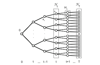
We consider a 1 -year planning horizon divided in the periods $t=0, \ldots, T$ corresponding to the trading dates. For each time $t$, we denote by $\mathcal{N} t$ the set of nodes at stage $t$. The root node is labeled with 0 and corresponds to the initial state. For $t \geq 1$ every $n \in \mathcal{N}{t}$ has a unique ancestor $a{n} \in \mathcal{N}{t-1}$, and for $t \leq T-1$ a non-empty set of child nodes $H{n} \in \mathcal{N}{t+1}$. We denote by $\mathcal{N}$ the whole set of nodes in the scenario tree. In addition, we refer by $t{n}$ the time stage of node $n$. A scenario is a path from the root to a leaf node and represents a joint realization of the random variables along the path to the planning horizon. We shall denote by $S$ the set of scenarios. Figure $4.1$ depicts an example scenario tree.
The scenario probability distribution $\mathcal{P}$ is defined on the leaf nodes of the scenario tree so that $\sum_{n \in N_{r}} p_{n}=1$ and for each non-terminal node $p_{n}=$ $\sum_{m \in H_{n}} p_{m}, \forall n \in N_{t}, t=T-1, \ldots, 0$, that is each node receives a conditional probability mass equal to the combined mass of all its descendant nodes. In our case study portfolio revisions imply a transition from the previous time $t-1$ portfolio allocation at the ancestor node to a new allocation through holding, buying, and selling decisions on individual securities, for $t=1, \ldots, T-1$. The last possible revision is at stage $T-1$ with one period to go. Consistent with the fixed-income portfolio problem, decisions are described by nominal, face-value, positions in the individual security $i \in I$ of rating class $k_{i} \in K$.
金融中的随机方法代写
统计代写|金融中的随机方法作业代写Stochastic Methods in Finance代考|Price–Yield Relationship
遵循 (4.7) 中的强度规范,单个证券在任何时候都可能受到将驱动证券进入默认状态的新信息的到来所归因的跳低违约事件的影响。增量价差行为与证券价格的关系如下。让默认进程的值dΨτ一世=1在随机时间τ. 然后,给定一个恢复值b一世, 我们有vτ,吨一世一世=∑τ<米≤吨一世C米一世和−b一世一世和−(r和+圆周率吨到一世)(米−τ)
在违约公告中,债券价格将反映在债券剩余期限内以固定风险贴现率贴现的所有付款的价值,包括无风险利率和类别到一世违约后的信用利差。所有评级类别的信用利差扩大将推高违约率,而不区分每个类别中的公司债券。另一方面,一旦在触发违约τ那么边际利差向上运动将被债券价格下跌所吸收,这与假设的回收率一致。
下列的(4.5)价格走势将取决于由以下因素引起的收益率跳跃这吨一世假设这与评级机构恢复估计的平均值一致(穆迪投资者服务公司 2009 年),并带有用户指定的不确定性,反映在具有随机跳跃大小的对数正态分布中b一世∼lnñ(μb一世,σb一世). 然后ln(b一世)∼ñ(μb一世,σb一世)以便b吨一世∈(0,+∞)和两者和−b一世(回收率)和1−和−b一世(损失率)属于区间(0,1).
综上所述,建模框架具有以下特点:
- 违约到达和违约损失的定义考虑了穆迪对特定评级的估计(2009)调整以考虑借款人的活动部门和市场违约溢价;
- 在 1 年的投资期限内,违约强度假设为常数,并将决定违约信息随机进入市场;违约时,边际价差将立即受到正向冲击,价格负向变动反映了证券在其剩余期限内不断部分支付;
- Poisson 过程和 Wiener 过程驱动独立的异质价差过程的行为,该过程假设与短期利率和信用价差过程共同确定证券价格动态;
- 每个评级等级的信用利差和短期利率是相关的。
该模型包含相关风险因素的假设,其行为将推动不同评级类别的所有证券,但包含特定的违约风险因素以区分每个类别中的证券行为。没有考虑传染现象,外生的价差动态会根据债券的久期和凸度结构影响特定的债券回报。
统计代写|金融中的随机方法作业代写Stochastic Methods in Finance代考|The Portfolio Value Process
我们现在扩展统计模型以描述在有限时间范围内影响投资组合价值动态的关键要素吨. 假设一个固定收益证券的投资范围具有年度票面利率,我们将在 1 年的范围内只有一次可能的票面支付和资本偿还。证券可能仅在这些时候违约并产生信用损失。我们猜测
由投资组合价值和现金账户在时间 0 定义的财富等式在0=∑到∈到∑一世∈一世到X一世0+C0, 在哪里X一世0是证券头寸的 time-0 市场价值一世, 由给定的名义投资产生X一世0并以目前的证券价格v0,吨一世一世. 为了吨=0,Δ吨,…,吨−Δ吨, 我们有
在吨+Δ吨,ω吨=∑到∈到∑一世∈HHX一世吨v一世,吨一世一世(1+ρ吨+Δ吨一世(ω))+C(吨+Δ吨,ω)
在 (4.9) 中,价格回报ρ吨+Δ吨一世根据 (4.5) 为每个证券生成v一世(吨+Δ吨,ω)v一世(吨)−1=[−d吨一世d是吨一世+是吨一世d吨+0.5C吨一世(d是吨一世)2], 在哪里是吨一世表示当时的收益率回报吨为了安全一世. 为了到=0我们有无违约类别,收益率将与无风险收益率一致。随着时间的推移,对信用损失进行评估。在与以前一样的年度时间跨度内,我们有
C(吨+Δ吨,ω)=C(吨)和r一世(ω)Δ吨+∑到∈到∑一世∈一世到C一世,吨+Δ吨+ −∑到∈到∑一世∈一世到C一世,吨+Δ吨(1−和[−b吨+Δ吨一世(ω)d在一世+Δ吨一世(ω)]).
现金余额C(吨)演变将取决于预期的现金流入C一世,吨以及每个头寸的相关信用损失一世, (4.10) 的第三个因子。(4.10) 中的息票和资本支付是根据特定证券的票面利率和到期日为给定的名义投资生成的。如果发生违约,那么对于给定的回收率,在计划范围内,投资者将面临(4.10)中的现金损失和(4.9)中的市场价值损失,这反映了在证券剩余时间跨度内持续部分支付的假设默认状态下。
等式(4.10)明确考虑了付款违约。但是,下面介绍的数学模型考虑了隐式默认损失定义。这是通过引入系数规范获得的
F一世,吨+Δ吨(ω)=C一世(和−[b一世+Δ吨一世(ω)dΨ一世+Δ一世一世一世(ω)])
因此,C一世,吨+Δ吨=X一世吨F一世,s+Δ吨, 在哪里C一世表示证券的票面利率一世.
在此框架中,公司债券经理将寻求最优动态策略,以寻求其投资组合的最高价格和现金回报,同时试图避免可能的违约损失。该模型非常通用,随机微分方程 (4.2)、(4.3) 和 (4.4) 的替代规范将导致不同的市场和损失情景,以适应未来可能出现的各种财富分布。
统计代写|金融中的随机方法作业代写Stochastic Methods in Finance代考|Dynamic Portfolio Model
在本节中,我们提出了一个适合制定和解决市场和信用风险控制问题的多阶段投资组合模型。人们普遍认为,随机规划提供了一种非常强大的范式,可以对所有以不确定性和动态性共同存在为特征的应用程序进行建模。在投资组合管理领域,随机规划已成功应用,近几十年出现的大量科学贡献证明了这一点(Bertocchi 等人 2007;Dempster 等人 2003;Hochreiter 和 Pflug 2007;Zenios 和 Ziemba 2007)。然而,很少有贡献在随机规划框架内处理信用和市场风险投资组合优化问题。这里我们提到 (Jobst et al.
然而,我们的模型与此相同,在目标函数中引入了风险回报权衡,以明确说明公司违约产生的不利影响。
我们考虑将 1 年的规划期限划分为多个时期吨=0,…,吨对应交易日。对于每一次吨,我们表示为ñ吨阶段的节点集吨. 根节点标记为 0,对应于初始状态。为了吨≥1每一个n∈ñ吨有一个独特的祖先一种n∈ñ吨−1,并且对于吨≤吨−1一组非空子节点Hn∈ñ吨+1. 我们表示ñ场景树中的整个节点集。另外,我们参考吨n节点时间阶段n. 场景是从根到叶节点的路径,表示沿路径到规划范围的随机变量的联合实现。我们将表示为小号场景集。数字4.1描绘了一个示例场景树。
情景概率分布磷在场景树的叶节点上定义,使得∑n∈ñrpn=1并且对于每个非终端节点pn= ∑米∈Hnp米,∀n∈ñ吨,吨=吨−1,…,0,即每个节点接收的条件概率质量等于其所有后代节点的组合质量。在我们的案例研究中,投资组合修订意味着与上一次的过渡吨−1通过对单个证券的持有、购买和出售决策,将祖先节点的投资组合分配到新的分配,吨=1,…,吨−1. 最后可能的修订是在阶段吨−1还有一段时期。与固定收益投资组合问题一致,决策由名义、面值、个人证券中的头寸来描述一世∈一世等级等级到一世∈到.

统计代写请认准statistics-lab™. statistics-lab™为您的留学生涯保驾护航。统计代写|python代写代考
随机过程代考
在概率论概念中,随机过程是随机变量的集合。 若一随机系统的样本点是随机函数,则称此函数为样本函数,这一随机系统全部样本函数的集合是一个随机过程。 实际应用中,样本函数的一般定义在时间域或者空间域。 随机过程的实例如股票和汇率的波动、语音信号、视频信号、体温的变化,随机运动如布朗运动、随机徘徊等等。
贝叶斯方法代考
贝叶斯统计概念及数据分析表示使用概率陈述回答有关未知参数的研究问题以及统计范式。后验分布包括关于参数的先验分布,和基于观测数据提供关于参数的信息似然模型。根据选择的先验分布和似然模型,后验分布可以解析或近似,例如,马尔科夫链蒙特卡罗 (MCMC) 方法之一。贝叶斯统计概念及数据分析使用后验分布来形成模型参数的各种摘要,包括点估计,如后验平均值、中位数、百分位数和称为可信区间的区间估计。此外,所有关于模型参数的统计检验都可以表示为基于估计后验分布的概率报表。
广义线性模型代考
广义线性模型(GLM)归属统计学领域,是一种应用灵活的线性回归模型。该模型允许因变量的偏差分布有除了正态分布之外的其它分布。
statistics-lab作为专业的留学生服务机构,多年来已为美国、英国、加拿大、澳洲等留学热门地的学生提供专业的学术服务,包括但不限于Essay代写,Assignment代写,Dissertation代写,Report代写,小组作业代写,Proposal代写,Paper代写,Presentation代写,计算机作业代写,论文修改和润色,网课代做,exam代考等等。写作范围涵盖高中,本科,研究生等海外留学全阶段,辐射金融,经济学,会计学,审计学,管理学等全球99%专业科目。写作团队既有专业英语母语作者,也有海外名校硕博留学生,每位写作老师都拥有过硬的语言能力,专业的学科背景和学术写作经验。我们承诺100%原创,100%专业,100%准时,100%满意。
机器学习代写
随着AI的大潮到来,Machine Learning逐渐成为一个新的学习热点。同时与传统CS相比,Machine Learning在其他领域也有着广泛的应用,因此这门学科成为不仅折磨CS专业同学的“小恶魔”,也是折磨生物、化学、统计等其他学科留学生的“大魔王”。学习Machine learning的一大绊脚石在于使用语言众多,跨学科范围广,所以学习起来尤其困难。但是不管你在学习Machine Learning时遇到任何难题,StudyGate专业导师团队都能为你轻松解决。
多元统计分析代考
基础数据: $N$ 个样本, $P$ 个变量数的单样本,组成的横列的数据表
变量定性: 分类和顺序;变量定量:数值
数学公式的角度分为: 因变量与自变量
时间序列分析代写
随机过程,是依赖于参数的一组随机变量的全体,参数通常是时间。 随机变量是随机现象的数量表现,其时间序列是一组按照时间发生先后顺序进行排列的数据点序列。通常一组时间序列的时间间隔为一恒定值(如1秒,5分钟,12小时,7天,1年),因此时间序列可以作为离散时间数据进行分析处理。研究时间序列数据的意义在于现实中,往往需要研究某个事物其随时间发展变化的规律。这就需要通过研究该事物过去发展的历史记录,以得到其自身发展的规律。
回归分析代写
多元回归分析渐进(Multiple Regression Analysis Asymptotics)属于计量经济学领域,主要是一种数学上的统计分析方法,可以分析复杂情况下各影响因素的数学关系,在自然科学、社会和经济学等多个领域内应用广泛。
MATLAB代写
MATLAB 是一种用于技术计算的高性能语言。它将计算、可视化和编程集成在一个易于使用的环境中,其中问题和解决方案以熟悉的数学符号表示。典型用途包括:数学和计算算法开发建模、仿真和原型制作数据分析、探索和可视化科学和工程图形应用程序开发,包括图形用户界面构建MATLAB 是一个交互式系统,其基本数据元素是一个不需要维度的数组。这使您可以解决许多技术计算问题,尤其是那些具有矩阵和向量公式的问题,而只需用 C 或 Fortran 等标量非交互式语言编写程序所需的时间的一小部分。MATLAB 名称代表矩阵实验室。MATLAB 最初的编写目的是提供对由 LINPACK 和 EISPACK 项目开发的矩阵软件的轻松访问,这两个项目共同代表了矩阵计算软件的最新技术。MATLAB 经过多年的发展,得到了许多用户的投入。在大学环境中,它是数学、工程和科学入门和高级课程的标准教学工具。在工业领域,MATLAB 是高效研究、开发和分析的首选工具。MATLAB 具有一系列称为工具箱的特定于应用程序的解决方案。对于大多数 MATLAB 用户来说非常重要,工具箱允许您学习和应用专业技术。工具箱是 MATLAB 函数(M 文件)的综合集合,可扩展 MATLAB 环境以解决特定类别的问题。可用工具箱的领域包括信号处理、控制系统、神经网络、模糊逻辑、小波、仿真等。