MATH 866 - 统计代写答疑辅导

标签： MATH 866

统计代写|金融中的随机方法作业代写Stochastic Methods in Finance代考| A 10-Year P&C ALM Problem

Posted on 2022年4月15日2022年4月15日 by statistics-lab

如果你也在怎样代写金融中的随机方法Stochastic Methods in Finance这个学科遇到相关的难题，请随时右上角联系我们的24/7代写客服。

随机建模是金融模型的一种形式，用于帮助做出投资决策。这种类型的模型使用随机变量预测不同条件下各种结果的概率。随着现代经济学、金融学实证研究的发展，金融中的随机方法Stochastic Methods in Finance作为一种数学工具具有越来越重要的应用价值。

statistics-lab™ 为您的留学生涯保驾护航在代写金融中的随机方法Stochastic Methods in Finance方面已经树立了自己的口碑, 保证靠谱, 高质且原创的统计Statistics代写服务。我们的专家在代写金融中的随机方法Stochastic Methods in Finance方面经验极为丰富，各种代写金融中的随机方法Stochastic Methods in Finance相关的作业也就用不着说。

我们提供的金融中的随机方法Stochastic Methods in Finance及其相关学科的代写，服务范围广, 其中包括但不限于:

Statistical Inference 统计推断
Statistical Computing 统计计算
Advanced Probability Theory 高等楖率论
Advanced Mathematical Statistics 高等数理统计学
(Generalized) Linear Models 广义线性模型
Statistical Machine Learning 统计机器学习
Longitudinal Data Analysis 纵向数据分析
Foundations of Data Science 数据科学基础

统计代写|金融中的随机方法作业代写Stochastic Methods in Finance代考|A 10-Year P&C ALM Problem

We present results for a test problem modelling a large $P \& C$ company assumed to manage a portfolio worth 10 billion $€$ (bln) at $t_{0}$. The firm’s management has set a first-year operating profit of 400 million $€(\mathrm{mln})$ and wishes to maximize in expectation the company realized and unrealized profits over 10 years. Company figures have been disguised for confidentiality reasons, though preserving the key elements of the original ALM problem. We name the P\&C company Danni Group.
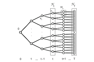
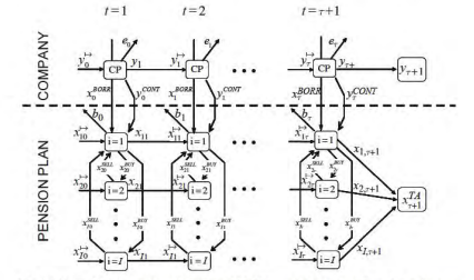
The following tree structure is assumed in this case study. The current implementable decision, corresponding to the root node, is set at 2 January 2010 (Table 5.4).

Within the model the $P \& C$ management will revise its strategy quarterly during the first year to minimize the expected shortfall with respect to the target.

Initial conditions in the problem formulation include average first-year insurance premiums $R(t)$ estimated at $4.2$ bln $€$, liability reserves $\Lambda(0)$ equal to $6.5$ bln $€$, and expected insurance claims $L(t)$ in the first year of $2.2$ bln $€$. The optimal investment policy, furthermore, is constrained by the following upper and lower bounds relative to the current portfolio value:

Bond portfolio upper bound: $85 \%$
Equity portfolio upper bound: $20 \%$
Corporate portfolio upper bound: $30 \%$
Real estate portfolio upper bound: $25 \%$
Desired turnover at rebalanced dates: $\leq 30 \%$
Cash lower bound: $5 \%$
The results that follow are generated through a set of software modules combining MATLAB $7.4 \mathrm{~b}$ as the main development tool, GAMS $21.5$ as the model generator and solution method provider, and Excel 2007 as the input and output data collector running under a Windows XP operating system with $1 \mathrm{~GB}$ of RAM and a dual processor.

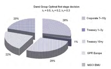
The objective function (5.1) of the P\&C ALM problem considers a tradeoff between short-, medium-, and long-term goals through the coefficients $\lambda_{1}=$ $0.5, \lambda_{2}=0.2$, and $\lambda_{3}=0.3$ at the 10-year horizon. The first coefficient determines a penalty on profit target shortfalls. The second and the third coefficients are associated, respectively, with a medium-term portfolio value decision criterion and long-term terminal wealth. Rebalancing decisions can be taken at decision epochs from time 0 up to the beginning of the last stage; no decisions are allowed at the horizon.

统计代写|金融中的随机方法作业代写Stochastic Methods in Finance代考|Optimal Investment Policy Under P&C Liability Constraints

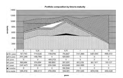
The optimal portfolio composition at time 0 , current time, the only one under full uncertainty regarding future financial scenarios, is displayed in Fig. 5.5.

Relying on a good liquidity buffer at time 0 the insurance manager will allocate wealth evenly across the asset classes with a similar portion of long Treasury and corporate bonds. As shown in Fig. $5.6$ the optimal strategy will then progressively

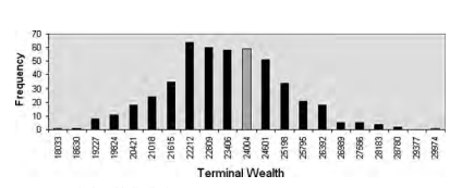
reduce holdings in equity and corporate bonds to increase the investment in Treasuries. A non-negligible real estate investment is kept throughout the 10 years. The allocation in the real estate index remains relatively stable as a result of the persistent company liquidity surplus. Real estate investments are overall preferred to equity investments due to higher expected returns per unit volatility estimated from the 1999 to 2009 historical sample. The optimal investment policy is characterized by quarterly rebalancing decisions during the first year with limited profit-taking operations allowed beyond the first business year. The 3 -year objective is primarily associated with the medium-term maximization of the portfolio asset value; the strategy will maximize unrealized portfolio gains specifically from long Treasury bonds, real estate, and corporate bonds. Over the 10 years the portfolio value moves along the average scenario from the initial 10 bln $€$ to roughly $14.3$ bln $€$.

The optimal portfolio strategy is not affected by the liquidity constraints from the technical side as shown in Table $5.5$. Danni Group has a strong liquidity buffer generated by the core insurance activity, but only sufficient on its own to reach the target profit set at the end of the first business year.

At the year I horizon the investment manager seeks to minimize the profit target shortfall while keeping all the upside. Indeed a $1.1$ billion $€$ gross profit is achieved prior to the corporate tax payment corresponding to roughly $750 \mathrm{mln}$ $€$ net profit. Thanks to the safe operational environment, no pressure is put on the investment side in terms of income generation and the investment manager is free to focus on the maximization of portfolio value at the 3-year horizon. Over the final 7-year stage the portfolio manager can be expected to concentrate on both realized and unrealized profit maximization, contributing to overall firm business growth, as witnessed in Table $5.5$ and Fig. 5.6. Empirical evidence suggests that P\&C optimal portfolio strategies, matching liabilities average life time, tend to concentrate on assets with limited duration (e.g. 1-3 years). We show below that such a strategy without an explicit risk capital constraint would penalize the portfolio terminal value.

统计代写|金融中的随机方法作业代写Stochastic Methods in Finance代考|Dynamic Asset Allocation with λ1 = 1

Remaining within a dynamic framework in the objective function (5.1) of the $P \& C$ ALM problem we set $\lambda_{1}=1$, with thus $\lambda_{2}=\lambda_{3}=0$ over the 10 -year horizon. The optimal policy will in this case be driven by the year 1 operating profit target, carrying on until the end of the decision horizon.

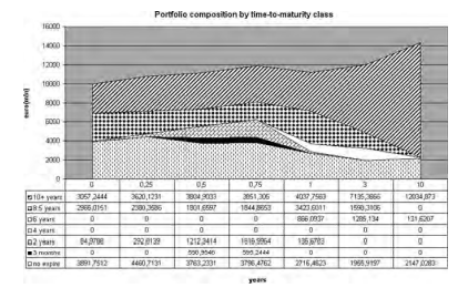
Diving a different view from Fig. 5.6, we display in Figs. $5.7$ and $5.8$ the optimal strategies in terms of the portfolio’s time-to-maturity structure in each stage. Relative to the portfolio composition in Fig. $5.8$ which corresponds to giving more weight to medium- and long-term objectives, the portfolio in Fig. $5.7$ concentrates from stage 1 on fixed income assets with lower duration. During the first year it shows an active rebalancing strategy and a more diversified portfolio. At the 9-month horizon part of the portfolio is liquidated and the resulting profit will minimize at the year 1 horizon the expected shortfall with respect to the target. Thereafter the strategy, suggesting a buy and hold management approach, will tend to concentrate on those assets that would not expire within the 10 -year horizon.

Consider now Fig. 5.8, recalling that no risk capital constraints are included in the model. The strategy remains relatively concentrated on long bonds and assets without a contractual maturity. Nevertheless the portfolio strategy is able to achieve the first target and heavily overperform over the 10 years. At $T=10$ years the first portfolio in this representative scenario is worth roughly $12.1$ billions $€$, while the second achieves a value of $14.2$ billions $€$.The year 1 horizon is the current standard for insurance companies seeking an optimal risk-reward trade-off typically within a static, one-period, framework. The above evidence suggests that over the same short-term horizon, a dynamic setting would in any case induce a more active strategy and, furthermore, a 10 -year extension of the decision horizon would not jeopardize the short-medium-term profitability of the P\&C shareholder while achieving superior returns in the long term.

金融中的随机方法代写

统计代写|金融中的随机方法作业代写Stochastic Methods in Finance代考|A 10-Year P&C ALM Problem

我们展示了一个测试问题的结果，它对一个大型模型进行了建模磷&C公司假定管理价值 100 亿美元的投资组合€€(bln) 在吨0. 公司管理层设定第一年营业利润为4亿€€(米一世n)并希望最大限度地期望公司在 10 年内实现和未实现的利润。尽管保留了原始 ALM 问题的关键要素，但出于保密原因对公司数据进行了伪装。我们将 P\&C 公司命名为 Danni Group。
在本案例研究中假设以下树结构。当前可执行的决策，对应于根节点，设置为 2010 年 1 月 2 日（表 5.4）。

在模型内磷&C管理层将在第一年每季度修订其战略，以尽量减少与目标相关的预期缺口。

问题表述中的初始条件包括平均首年保费R(吨)估计在4.2月€€, 负债准备金Λ(0)等于6.5月€€，以及预期的保险索赔大号(吨)在第一年2.2月€€. 此外，最佳投资政策受以下相对于当前投资组合价值的上限和下限的约束：

债券组合上限：85%
股票投资组合上限：20%
企业投资组合上限：30%
房地产投资组合上限：25%
重新平衡日期的期望营业额：≤30%
现金下限：5%
下面的结果是通过一组结合MATLAB的软件模块生成的7.4 b作为主要的开发工具，GAMS21.5作为模型生成器和求解方法提供者，Excel 2007 作为输入和输出数据收集器，在 Windows XP 操作系统下运行1 G乙RAM 和双处理器。

P\&C ALM 问题的目标函数 (5.1) 通过系数考虑了短期、中期和长期目标之间的权衡λ1= 0.5,λ2=0.2，和λ3=0.3在 10 年的范围内。第一个系数确定对利润目标不足的惩罚。第二和第三个系数分别与中期投资组合价值决策标准和长期终端财富相关联。可以在从时间 0 到最后阶段开始的决策时期进行再平衡决策；不允许在地平线上做出任何决定。

统计代写|金融中的随机方法作业代写Stochastic Methods in Finance代考|Optimal Investment Policy Under P&C Liability Constraints

图 5.5 显示了当前时间 0 时的最优投资组合构成，这是未来金融情景中唯一完全不确定的投资组合。

依靠时间 0 的良好流动性缓冲，保险经理将在资产类别中平均分配财富，并持有类似比例的长期国债和公司债券。如图所示。5.6最优策略将逐渐

减持股票和公司债券，增加对国债的投资。在整个 10 年中保持着不可忽略的房地产投资。由于公司流动性持续过剩，房地产指数的配置保持相对稳定。由于从 1999 年到 2009 年的历史样本估计的每单位波动率的预期回报较高，房地产投资总体上优于股权投资。最佳投资政策的特点是在第一年进行季度再平衡决策，在第一年之后允许有限的获利了结操作。3 年目标主要与投资组合资产价值的中期最大化有关；该策略将最大化未实现的投资组合收益，特别是来自长期国债、房地产、和公司债券。在 10 年中，投资组合价值从最初的 100 亿美元沿着平均情景移动€€大致地14.3月€€.

最优组合策略不受技术面流动性约束的影响，如表所示5.5. Danni Group 拥有由核心保险业务产生的强大流动性缓冲，但仅靠其自身就足以达到第一财年末设定的目标利润。

在我眼中的那一年，投资经理力求将利润目标缺口最小化，同时保持所有上涨空间。确实一个1.1十亿€€毛利是在缴纳企业税之前实现的，大致相当于750米一世n €€净利。得益于安全的运营环境，投资方在创收方面没有压力，投资经理可以在 3 年内专注于投资组合价值的最大化。在最后 7 年阶段，可以预期投资组合经理将专注于已实现和未实现的利润最大化，为公司的整体业务增长做出贡献，如表所示5.5和图 5.6。经验证据表明，P\&C 最优投资组合策略，匹配负债平均寿命，往往集中在有限期限（例如 1-3 年）的资产上。我们在下面展示了这种没有明确风险资本约束的策略会惩罚投资组合的终值。

统计代写|金融中的随机方法作业代写Stochastic Methods in Finance代考|Dynamic Asset Allocation with λ1 = 1

保持在目标函数（5.1）的动态框架内磷&C我们设置的 ALM 问题λ1=1, 因此λ2=λ3=0在 10 年的范围内。在这种情况下，最优政策将由第 1 年的营业利润目标驱动，一直持续到决策期限结束。

潜水与图 5.6 不同的视图，我们显示在图 5.6 中。5.7和5.8根据投资组合在每个阶段的到期时间结构的最优策略。相对于图 1 中的投资组合构成。5.8这对应于给予中长期目标更多的权重，图 3 中的投资组合。5.7从第 1 阶段开始，专注于期限较短的固定收益资产。在第一年，它显示出积极的再平衡策略和更加多元化的投资组合。在 9 个月范围内，部分投资组合被清算，由此产生的利润将在第 1 年范围内最小化与目标相关的预期缺口。此后，建议采取买入并持有管理方法的策略将倾向于专注于那些不会在 10 年内到期的资产。

现在考虑图 5.8，回顾模型中没有包含风险资本约束。该策略仍然相对集中于长期债券和没有合同到期的资产。尽管如此，投资组合策略还是能够实现第一个目标，并且在 10 年内表现出色。在吨=10年这个代表性场景中的第一个投资组合价值大约12.1数十亿€€，而第二个达到的值14.2数十亿€€. 第 1 年范围是保险公司寻求最佳风险回报权衡的当前标准，通常是在静态的单周期框架内。上述证据表明，在相同的短期范围内，动态环境无论如何都会引发更积极的战略，此外，决策范围延长 10 年不会危及公司的中短期盈利能力。 P\&C 股东，同时实现长期超额回报。

统计代写|金融中的随机方法作业代写Stochastic Methods in Finance代考请认准statistics-lab™

统计代写请认准statistics-lab™. statistics-lab™为您的留学生涯保驾护航。统计代写|python代写代考

随机过程代考

在概率论概念中，随机过程是随机变量的集合。若一随机系统的样本点是随机函数，则称此函数为样本函数，这一随机系统全部样本函数的集合是一个随机过程。实际应用中，样本函数的一般定义在时间域或者空间域。 随机过程的实例如股票和汇率的波动、语音信号、视频信号、体温的变化，随机运动如布朗运动、随机徘徊等等。

贝叶斯方法代考

贝叶斯统计概念及数据分析表示使用概率陈述回答有关未知参数的研究问题以及统计范式。后验分布包括关于参数的先验分布，和基于观测数据提供关于参数的信息似然模型。根据选择的先验分布和似然模型，后验分布可以解析或近似，例如，马尔科夫链蒙特卡罗 (MCMC) 方法之一。贝叶斯统计概念及数据分析使用后验分布来形成模型参数的各种摘要，包括点估计，如后验平均值、中位数、百分位数和称为可信区间的区间估计。此外，所有关于模型参数的统计检验都可以表示为基于估计后验分布的概率报表。

广义线性模型代考

广义线性模型（GLM）归属统计学领域，是一种应用灵活的线性回归模型。该模型允许因变量的偏差分布有除了正态分布之外的其它分布。

statistics-lab作为专业的留学生服务机构，多年来已为美国、英国、加拿大、澳洲等留学热门地的学生提供专业的学术服务，包括但不限于Essay代写，Assignment代写，Dissertation代写，Report代写，小组作业代写，Proposal代写，Paper代写，Presentation代写，计算机作业代写，论文修改和润色，网课代做，exam代考等等。写作范围涵盖高中，本科，研究生等海外留学全阶段，辐射金融，经济学，会计学，审计学，管理学等全球99%专业科目。写作团队既有专业英语母语作者，也有海外名校硕博留学生，每位写作老师都拥有过硬的语言能力，专业的学科背景和学术写作经验。我们承诺100%原创，100%专业，100%准时，100%满意。

机器学习代写

随着AI的大潮到来，Machine Learning逐渐成为一个新的学习热点。同时与传统CS相比，Machine Learning在其他领域也有着广泛的应用，因此这门学科成为不仅折磨CS专业同学的“小恶魔”，也是折磨生物、化学、统计等其他学科留学生的“大魔王”。学习Machine learning的一大绊脚石在于使用语言众多，跨学科范围广，所以学习起来尤其困难。但是不管你在学习Machine Learning时遇到任何难题，StudyGate专业导师团队都能为你轻松解决。

多元统计分析代考

基础数据: $N$ 个样本， $P$ 个变量数的单样本，组成的横列的数据表
变量定性: 分类和顺序；变量定量：数值
数学公式的角度分为: 因变量与自变量

时间序列分析代写

随机过程，是依赖于参数的一组随机变量的全体，参数通常是时间。随机变量是随机现象的数量表现，其时间序列是一组按照时间发生先后顺序进行排列的数据点序列。通常一组时间序列的时间间隔为一恒定值（如1秒，5分钟，12小时，7天，1年），因此时间序列可以作为离散时间数据进行分析处理。研究时间序列数据的意义在于现实中，往往需要研究某个事物其随时间发展变化的规律。这就需要通过研究该事物过去发展的历史记录，以得到其自身发展的规律。

回归分析代写

多元回归分析渐进（Multiple Regression Analysis Asymptotics）属于计量经济学领域，主要是一种数学上的统计分析方法，可以分析复杂情况下各影响因素的数学关系，在自然科学、社会和经济学等多个领域内应用广泛。

MATLAB代写

MATLAB 是一种用于技术计算的高性能语言。它将计算、可视化和编程集成在一个易于使用的环境中，其中问题和解决方案以熟悉的数学符号表示。典型用途包括：数学和计算算法开发建模、仿真和原型制作数据分析、探索和可视化科学和工程图形应用程序开发，包括图形用户界面构建MATLAB 是一个交互式系统，其基本数据元素是一个不需要维度的数组。这使您可以解决许多技术计算问题，尤其是那些具有矩阵和向量公式的问题，而只需用 C 或 Fortran 等标量非交互式语言编写程序所需的时间的一小部分。MATLAB 名称代表矩阵实验室。MATLAB 最初的编写目的是提供对由 LINPACK 和 EISPACK 项目开发的矩阵软件的轻松访问，这两个项目共同代表了矩阵计算软件的最新技术。MATLAB 经过多年的发展，得到了许多用户的投入。在大学环境中，它是数学、工程和科学入门和高级课程的标准教学工具。在工业领域，MATLAB 是高效研究、开发和分析的首选工具。MATLAB 具有一系列称为工具箱的特定于应用程序的解决方案。对于大多数 MATLAB 用户来说非常重要，工具箱允许您学习和应用专业技术。工具箱是 MATLAB 函数（M 文件）的综合集合，可扩展 MATLAB 环境以解决特定类别的问题。可用工具箱的领域包括信号处理、控制系统、神经网络、模糊逻辑、小波、仿真等。

R语言代写	问卷设计与分析代写
PYTHON代写	回归分析与线性模型代写
MATLAB代写	方差分析与试验设计代写
STATA代写	机器学习/统计学习代写
SPSS代写	计量经济学代写
EVIEWS代写	时间序列分析代写
EXCEL代写	深度学习代写
SQL代写	各种数据建模与可视化代写

统计代写|金融中的随机方法作业代写Stochastic Methods in Finance代考| Scenario Generation

Posted on 2022年4月15日2022年4月15日 by statistics-lab

如果你也在怎样代写金融中的随机方法Stochastic Methods in Finance这个学科遇到相关的难题，请随时右上角联系我们的24/7代写客服。

我们提供的金融中的随机方法Stochastic Methods in Finance及其相关学科的代写，服务范围广, 其中包括但不限于:

Statistical Inference 统计推断
Statistical Computing 统计计算
Advanced Probability Theory 高等楖率论
Advanced Mathematical Statistics 高等数理统计学
(Generalized) Linear Models 广义线性模型
Statistical Machine Learning 统计机器学习
Longitudinal Data Analysis 纵向数据分析
Foundations of Data Science 数据科学基础

统计代写|金融中的随机方法作业代写Stochastic Methods in Finance代考|Scenario Generation

The optimal ALM strategy in the model depends on an extended set of asset and liability processes. We assume a multivariate normal distribution for monthly price returns of a representative set of market benchmarks including fixed income, equity, and real estate indices. The following $I=12$ investment opportunities are considered: for $i=1$ : the EURIBOR 3 months; for $i=2,3,4,5$, 6: the Barclays Treasury indices for maturity buckets $1-3,3-5,5-7,7-10$, and $10+$ years, respectively; for $i=7,8,9,10$ : the Barclays Corporate indices, again spanning maturities $1-3,3-5,5-7$, and $7-10$ years; finally for $i=11$ : the GPR Real Estate Europe index and $i=12$ : the MSCI EMU equity index. Recall that in our notation $I_{1}$ includes all fixed income assets and $I_{2}$ the real estate and equity investments.

The benchmarks represent total return indices incorporating over time the securities’ cash payments. In the definition of the strategic asset allocation problem, unlike
5 Dynamic Portfolio Management for Property and Casualty Insuranee
109
real estate and equity investments, money market and fixed income benchmarks are assumed to have a fixed maturity equal to their average duration ( 3 months, 2 years, 4,6 , and $8.5$ years for the corresponding Treasury and Corporate indices and 12 years for the $10+$ Treasury index). Income cashflows due to coupon payments will be estimated ex post through an approximation described below upon selling or expiry of fixed income benchmarks and disentangled from price returns. Equity investments will instead generate annual dividends through a price-adjusted random dividend yield. Finally, for real estate investments a simple model focusing only on price returns is considered. Scenario generation translates the indices return trajectories for the above market benchmarks into a tree process (see, for instance, the tree structure in Fig. 5.3) for the ALM coefficients (Consigli et al., 2010; Chapters 15 and 16 ): this is referred to in the sequel as the tree coefficient process. We rely on the process nodal realizations (Chapter 4 ) to identify the coefficients to be associated with each decision variable in the ALM model. We distinguish in the decision model between asset and liability coefficients.

统计代写|金融中的随机方法作业代写Stochastic Methods in Finance代考|Asset Return Scenarios

The following random coefficients must be derived from the data process simulations along the specified scenario tree. For each scenario $s$, at $t=t_{0}, t_{1}, \ldots, t_{n}=H$, we define
$\rho_{i, t}(s)$ : the return of asset $i$ at time $t$ in scenario $s$;
$\delta_{i, t}(s)$ : the dividend yield of asset $i$ at time $t$ in scenario $s$;
$\eta_{i, h, t}(s)$ : a positive interest at time $t$ in scenario $s$ per unit investment in asset $i \in I_{1}$, in epoch $h$;
$\gamma_{i, h, t}(s)$ : the capital gain at time $t$ in scenario $s$ per unit investment in asset $i \in I_{2}$ in epoch $h$;
$\zeta_{t}^{+/-}(s):$ the (positive and negative) interest rates on the cash account at time $t$ in scenario $s$.

Price refurns $\rho_{i, t}(s)$ under scenario s are directly computed from the associated benchmarks $V_{i, t}(s)$ assuming a multivariate normal distribution, with $\rho:=$ $\left{\rho_{i}(\omega)\right}, \rho \sim N(\mu, \Sigma)$, where $\omega$ denotes a generic random element, and $\mu$ and $\Sigma$ denote the return mean vector and variance-covariance matrix, respectively. In the statistical model we consider for $i \in I 12$ investment opportunities and the inflation rate. Denoting by $\Delta t$ a monthly time increment and given the initial values $V_{i, 0}$ for $i=1,2, \ldots, 12$, we assume a stochastic difference equation for $V_{i, t}:$
$$
\begin{aligned}
\rho_{i, t}(s) &=\frac{V_{i, t}(s)-V_{i, t-\Delta t}(s)}{V_{i, t}-\Delta t(s)}, \
\frac{\Delta V_{i, t}(s)}{V_{i, t}(s)}=\mu \Delta t+\Sigma \Delta W_{t}(s) .
\end{aligned}
$$

In $(5.12), \Delta W_{t} \sim N(0, \Delta t)$. We show in Tables $5.2$ and $5.3$ the estimated statistical parameters adopted to generate through Monte Carlo simulation (Consigli et al., 2010 ; Glasserman, 2003 ) the correlated monthly returns in (5.12) for each benchmark $i$ and scenario $s$. Monthly returns are then compounded according to the horizon partition (see Fig. 5.1) following a prespecified scenario tree structure. The return scenarios in tree form are then passed on to an algebraic language deterministic model generator to produce the stochastic program deterministic equivalent instance (Consigli and Dempster, 1998).

Equity dividends are determined independently in terms of the equity position at the beginning of a stage as $\sum_{i \in l_{2}} x_{i, f_{j-1}}(s) \delta_{i, t_{j}}(s)$, where $\delta_{i, t_{j}}(s) \sim N(0.02,0.005)$ is the dividend yield.

Interest margin $M_{t_{j}}(s)=I_{t_{j}}^{+}(s)-I_{t_{j}}^{-}(s)$ is computed by subtracting negative from positive interest cash flows. Negative interest $I_{t_{j}}^{-}(s)=z_{t_{j-1}}^{-}(s) \zeta_{t_{j}}^{-}(s)$ is generated by short positions on the current account according to a fixed $2 \%$ spread over the Euribor 3 -month rate for the current period. The positive interest rate for cash surplus is fixed at $\zeta^{+}(t, s)=0.5 \%$ for all $t$ and $s$.

Positive interest $I_{t_{j}}^{+}(s)$ is calculated from return scenarios of fixed income investments $i \in I_{2}$ using buying-selling price differences assuming initial unit investments; this may be regarded as a suitable first approximation. In the case of negative price differences, the loss is entirely attributed to price movements and the interest accrual is set to 0 .
We recognize that this is a significant simplifying assumption. It is adopted here to avoid the need for an explicit yield curve model, whose introduction would go beyond the scope of a case study. Nevertheless we believe that this simplification allows one to recognize the advantages of a dynamic version of the portfolio management problem.

统计代写|金融中的随机方法作业代写Stochastic Methods in Finance代考|Liability Scenarios

Annual premium renewals by P\&C policyholders represent the key technical income on which the company relies for its ongoing business requirements. Premiums have associated random insurance claims over the years and, depending on the business cycle and the claim class, they might induce different reserve requirements. The latter constitute the insurance company’s most relevant liability. In our analysis premiums are assumed to be written annually and will be stationary over the 10-year horizon with limited volatility. Insurance claims are also assumed to remain stable over time in nominal terms, but with an inflation adjustment that in the long term may affect the company’s short-term liquidity. For a given estimate of insurance premiums $R_{0}$ collected in the first year, along scenario $s$, for $t=t_{1}, t_{2}, \ldots, H$, with $e_{r} \sim N(1,0.03)$, we assume that
$$
R_{t j}(s)=\left[R_{t j-1}(s) \cdot e_{r}\right] .
$$
Insurance claims are assumed to grow annually at the inflation rate and in nominal terms are constant in expectation. For given initial liability $L_{0}$, with $e_{l} \sim$ $N(1,0.01)$
$$
L_{t_{j}}(s)=\left(L_{t_{j-1}}(s) \cdot e t\right)\left(1+\pi_{t_{j}}(s)\right) .
$$
Every year the liability stream is assumed to vary in the following year according to a normal distribution with the previous year’s mean and a $1 \%$ volatility per year with a further inflation adjustment. Given $\pi(0)$ at time 0 , the inflation process $\pi_{t}(s)$ is assumed to follow a mean-reverting process

$$
\Delta \pi_{t}(s)=\alpha_{\pi}\left(\mu-\pi_{t}(s)\right) \Delta t+\sigma_{\pi} \Delta W_{t}(s)
$$
with $\mu$ set in our case study to the $2 \%$ European central bank target and $\Delta W_{t} \cdots$ $N(0, \Delta t)$. As for the other liability variables technical resenves are computed as a linear function of the current liability as $\Lambda_{t}(s)=L_{t}(s) \cdot \lambda$, where $\lambda$ in our case study is approximated by $1 / 0.3$ as estimated by practitioner opinion.

Operational costs $C_{t_{j}}(s)$ include staff and back-office and are assumed to increase at the inflation rate. For a given initial estimate $C_{0}$, along each scenario and stage, we have
$$
C_{t_{j}}(s)=C_{t_{j-1}}(s) \cdot\left(1+\pi_{t_{j}}(s)\right)
$$
Bad liability scenarios will be induced by years of premium reductions associated with unexpected insurance claim increases, leading to higher reserve requirements that, in turn, would require a higher capital base. A stressed situation is discussed in Section $5.4$ to emphasize the flexibility of dynamic strategies to adapt to bad technical scenarios and compensate for such losses. The application also shows that within a dynamic framework the insurance manager is able to achieve an optimal trade-off between investment and technical profit generation across scenarios and over time, and between risky and less risky portfolio positions.

金融中的随机方法代写

统计代写|金融中的随机方法作业代写Stochastic Methods in Finance代考|Scenario Generation

模型中的最优 ALM 策略取决于一组扩展的资产和负债流程。我们假设一组具有代表性的市场基准（包括固定收益、股票和房地产指数）的月价格回报呈多元正态分布。以下一世=12考虑投资机会：一世=1: EURIBOR 3 个月; 为了一世=2,3,4,5, 6: 到期桶的巴克莱国库指数1−3,3−5,5−7,7−10，和10+年，分别；为了一世=7,8,9,10：巴克莱公司指数，再次跨越期限1−3,3−5,5−7，和7−10年; 终于为一世=11：GPR 房地产欧洲指数和一世=12: MSCI EMU 股票指数。回想一下，在我们的符号中一世1包括所有固定收益资产和一世2房地产和股权投资。

基准代表总回报指数，包括随着时间的推移证券的现金支付。在战略资产配置问题的定义中，与
5 财产险和意外险的动态投资组合管理
109
房地产和股权投资不同，假设货币市场和固定收益基准的固定期限等于它们的平均久期（3 个月，2年，4,6 和8.5相应的国库券和公司指数为 12 年，10+国库指数）。因支付息票而产生的收入现金流量将通过以下在固定收益基准出售或到期时描述的近似值进行事后估计，并与价格回报脱钩。相反，股权投资将通过价格调整后的随机股息收益率产生年度股息。最后，对于房地产投资，我们考虑了一个只关注价格回报的简单模型。情景生成将上述市场基准的指数回报轨迹转换为 ALM 系数的树形过程（例如，参见图 5.3 中的树形结构）（Consigli 等人，2010；第 15 章和第 16 章）：这是后面称为树系数过程。我们依靠过程节点实现（第 4 章）来识别与 ALM 模型中的每个决策变量相关联的系数。我们在决策模型中区分资产和负债系数。

统计代写|金融中的随机方法作业代写Stochastic Methods in Finance代考|Asset Return Scenarios

以下随机系数必须从沿指定场景树的数据过程模拟中得出。对于每个场景s，在吨=吨0,吨1,…,吨n=H，我们定义
ρ一世,吨(s): 资产回报一世有时吨在情景中s;
d一世,吨(s): 资产的股息收益率一世有时吨在情景中s;
这一世,H,吨(s): 对时间的积极兴趣吨在情景中s单位资产投资一世∈一世1, 在纪元H;
C一世,H,吨(s)：当时的资本收益吨在情景中s单位资产投资一世∈一世2在时代H;
G吨+/−(s):现金账户当时的（正和负）利率吨在情景中s.

价格返还ρ一世,吨(s)场景下的 s 直接从相关的基准计算五一世,吨(s)假设一个多元正态分布，ρ:= \left{\rho_{i}(\omega)\right}, \rho \sim N(\mu, \Sigma)\left{\rho_{i}(\omega)\right}, \rho \sim N(\mu, \Sigma)，在哪里ω表示一个通用随机元素，并且μ和Σ分别表示返回均值向量和方差-协方差矩阵。在我们考虑的统计模型中一世∈一世12投资机会和通货膨胀率。表示Δ吨每月时间增量并给定初始值五一世,0为了一世=1,2,…,12，我们假设一个随机差分方程五一世,吨:
ρ一世,吨(s)=五一世,吨(s)−五一世,吨−Δ吨(s)五一世,吨−Δ吨(s), Δ五一世,吨(s)五一世,吨(s)=μΔ吨+ΣΔ在吨(s).

在(5.12),Δ在吨∼ñ(0,Δ吨). 我们在表格中显示5.2和5.3通过蒙特卡罗模拟（Consigli 等人，2010 年；Glasserman，2003 年）生成的估计统计参数每个基准在 (5.12) 中的相关月收益一世和场景s. 然后按照预先指定的情景树结构，根据水平分区（见图 5.1）对月回报进行复合。然后将树形式的返回场景传递给代数语言确定性模型生成器，以生成随机程序确定性等效实例（Consigli 和 Dempster，1998 年）。

股权分红根据阶段开始时的股权状况独立确定∑一世∈一世2X一世,Fj−1(s)d一世,吨j(s)，在哪里d一世,吨j(s)∼ñ(0.02,0.005)是股息收益率。

息差米吨j(s)=一世吨j+(s)−一世吨j−(s)通过从正利息现金流中减去负数来计算。负利率一世吨j−(s)=和吨j−1−(s)G吨j−(s)是由经常账户的空头头寸根据固定的2%分布在当前期间的 3 个月 Euribor 利率上。现金盈余的正利率固定为G+(吨,s)=0.5%对全部吨和s.

积极的兴趣一世吨j+(s)根据固定收益投资的回报方案计算一世∈一世2假设初始单位投资，使用买卖价格差异；这可以被认为是一个合适的第一近似值。在负价格差异的情况下，损失完全归因于价格变动，应计利息设置为 0。
我们认识到这是一个重要的简化假设。这里采用它是为了避免需要明确的收益率曲线模型，其引入将超出案例研究的范围。尽管如此，我们相信这种简化可以让人们认识到动态版本的投资组合管理问题的优势。

统计代写|金融中的随机方法作业代写Stochastic Methods in Finance代考|Liability Scenarios

财产险保单持有人的年度保费续保代表了公司依赖其持续业务需求的关键技术收入。多年来，保费与随机保险索赔相关，并且根据商业周期和索赔类别，它们可能会导致不同的准备金要求。后者构成保险公司最相关的责任。在我们的分析中，假设保费为每年一次，并且在 10 年内保持稳定，波动性有限。保险索赔也被假设在名义上随着时间的推移保持稳定，但通货膨胀调整从长远来看可能会影响公司的短期流动性。对于给定的保险费估计R0第一年收集，沿情景s，为了吨=吨1,吨2,…,H，和和r∼ñ(1,0.03), 我们假设
R吨j(s)=[R吨j−1(s)⋅和r].
假设保险索赔每年以通货膨胀率增长，并且名义上的预期是不变的。对于给定的初始责任大号0，和和一世∼ ñ(1,0.01)
大号吨j(s)=(大号吨j−1(s)⋅和吨)(1+圆周率吨j(s)).
假设每年的负债流在下一年按照正态分布变化，上一年的平均值和1%随着通货膨胀的进一步调整，每年波动。给定圆周率(0)在时间 0 ，膨胀过程圆周率吨(s)假设遵循均值回复过程Δ圆周率吨(s)=一种圆周率(μ−圆周率吨(s))Δ吨+σ圆周率Δ在吨(s)
和μ在我们的案例研究中设置为2%欧洲央行目标和Δ在吨⋯ ñ(0,Δ吨). 至于其他负债变量，技术收益被计算为当前负债的线性函数Λ吨(s)=大号吨(s)⋅λ，在哪里λ在我们的案例研究中，近似于1/0.3根据从业者的意见估计。

运营成本C吨j(s)包括员工和后台，并假设随着通货膨胀率增加。对于给定的初始估计C0，在每个场景和阶段，我们有
C吨j(s)=C吨j−1(s)⋅(1+圆周率吨j(s))
与意外保险索赔增加相关的多年保费减少将引发不良责任情景，从而导致更高的准备金要求，进而需要更高的资本基础。第一部分讨论了压力情况5.4强调动态策略的灵活性，以适应糟糕的技术情景并弥补此类损失。该应用程序还表明，在动态框架内，保险经理能够在不同场景和一段时间内以及在风险和风险较低的投资组合头寸之间实现投资和技术利润产生之间的最佳权衡。

统计代写请认准statistics-lab™. statistics-lab™为您的留学生涯保驾护航。统计代写|python代写代考

随机过程代考

贝叶斯方法代考

广义线性模型代考

广义线性模型（GLM）归属统计学领域，是一种应用灵活的线性回归模型。该模型允许因变量的偏差分布有除了正态分布之外的其它分布。

机器学习代写

多元统计分析代考

基础数据: $N$ 个样本， $P$ 个变量数的单样本，组成的横列的数据表
变量定性: 分类和顺序；变量定量：数值
数学公式的角度分为: 因变量与自变量

时间序列分析代写

回归分析代写

MATLAB代写

R语言代写	问卷设计与分析代写
PYTHON代写	回归分析与线性模型代写
MATLAB代写	方差分析与试验设计代写
STATA代写	机器学习/统计学习代写
SPSS代写	计量经济学代写
EVIEWS代写	时间序列分析代写
EXCEL代写	深度学习代写
SQL代写	各种数据建模与可视化代写

统计代写|金融中的随机方法作业代写Stochastic Methods in Finance代考| The ALM Model

Posted on 2022年4月15日2022年4月15日 by statistics-lab

如果你也在怎样代写金融中的随机方法Stochastic Methods in Finance这个学科遇到相关的难题，请随时右上角联系我们的24/7代写客服。

我们提供的金融中的随机方法Stochastic Methods in Finance及其相关学科的代写，服务范围广, 其中包括但不限于:

Statistical Inference 统计推断
Statistical Computing 统计计算
Advanced Probability Theory 高等楖率论
Advanced Mathematical Statistics 高等数理统计学
(Generalized) Linear Models 广义线性模型
Statistical Machine Learning 统计机器学习
Longitudinal Data Analysis 纵向数据分析
Foundations of Data Science 数据科学基础

Marketing Management: A Systems Framework (2) | by Christie Nordhielm PhD | Marketing Management: A Systems Framework | Medium — 统计代写|金融中的随机方法作业代写Stochastic Methods in Finance代考| The ALM Model

统计代写|金融中的随机方法作业代写Stochastic Methods in Finance代考|The ALM Model

The ALM problem is formulated as a linear MSP recourse problem (Birge and Louveaux, 1997; Consigli 2007; Consigli and Dempster, 1998) over six stages. The optimal root node decision is taken at time $t_{0}=0$ and, from a practical viewpoint, represents the key implementable decision. Recourse decisions occur at $t_{1}=0.25$ (after a quarter), $t_{2}=0.5, t_{3}=0.75, t_{4}=1$ year, and $t_{5}=3$ years. The objective function includes a first-year profit shortfall with respect to a target (at $\left.t_{4}\right)$, a 3-year expected excess portfolio value relative to the insurance reserves (at $\left.t_{5}\right)$, and a 10-year wealth objective (at $t_{6}=H$ ):
$$
\max {x \in X}\left{-\lambda{1} E\left[\tilde{\Pi}{t 4}-\Pi{t 4} \mid \Pi_{t 4}<\tilde{\Pi}{t 4}\right]+\lambda{2} E\left(X_{t 5}-\Lambda_{t 5}\right)+\lambda_{3} E\left[W_{H}\right]\right}
$$
with $\lambda_{1}+\lambda_{2}+\lambda_{3}=1,0 \leq \lambda_{1}, \lambda_{2}, \lambda_{3} \leq 1$.
The first-year horizon reflects the short-term objective to be achieved at the end of the current year: a target net profit is included and for given liabilities and random cash flows over the initial four quarters the model will tend to minimize the expected shortfall with respect to the target (Artzner et al., 1999; Rockafellar and Uryasev, 2002). The intermediate 3 -year objective reflects the maximization of the investment portfolio value above the $\mathrm{P} \& \mathrm{C}$ liabilities. The 10-year expected terminal wealth objective, finally, reflects management’s need to maximize on average the long-term realized and unrealized profits.

The prospective optimal strategy is determined as a set of scenario-dependent decisions to maximize this objective function subject to several constraints. Decision variables include holding, selling, and buying indices in a representative strategic investment universe. We distinguish the set $i \in I_{1}$, including all interest-bearing assets with a specified maturity, from $i \in I_{2}$, which includes real estate and equity assets without an expiry date. The asset universe is $I=I_{1} \cup I_{2}$ :

$x^{+}(i, t, s)$ imestment in stage $t$, scenario $s$, of asset $i$ (with maturity $T_{i}$ for $\left.i \in I_{1}\right)$;
$x^{-}(i, h, t, s)$ selling in stage $t$, scenario $s$, of asset $i$ (with maturity $T_{i}$ for $i \in I_{1}$ ) that was bought in $h$;
$x^{\exp }(i, h, t, s)$ maturity in stage $t$, scenario $s$, of asset $i \in I_{1}$ that was bought in $h$;
$x(i, h, t, s)$ holding in stage $t$, scenario $s$, of asset $i$ (with maturity $T_{i}$ for $i \in I_{1}$ ) that was bought in $h$;
$z(t, s)=z^{+}(t, s)-z^{-}(t, s)$ cash account in stage $t$, scenario $s$.
The investmént epoochs $h=t_{0}, l_{1}, \ldots, t_{n-1} \mathrm{~ a ̈ r e ̀ ~ a ̊ l s o ~ i n t r o ̛ d u c e ́ d ~ i n ~ o ̛ r d e ́ r ~ t o}$ mate the capital gains on specific investments. An extended set of linear constraints will determine the feasibility region of the SP problem (Birge and Louveaux, 1997; Consigli and Dempster, 1998).

统计代写|金融中的随机方法作业代写Stochastic Methods in Finance代考|Inventory Balance Constraints

The inventory balance constraints affect the time evolution of the asset portfolio. Given an initial input portfolio the constraints take care of the stage evolution of the optimal strategy. Starting at time 0 we model the market value of the investment at each node along a scenario, for each asset class $i$. Unlike real estate and equity investments, fixed income portfolio holdings are assumed to carry a maturity date. At time 0 an initial input portfolio $x_{i}$, prior to any rebalancing decision, is assumed. We distinguish between the initial time 0 constraints and those for the later stages:
$$
\begin{aligned}
x_{i, 0} &=\stackrel{\circ}{x}{i}+x{i, 0}^{+}-x_{i, 0}^{-} \quad \forall i \in I \
X_{0} &=\sum_{i \in I} x_{i, 0}
\end{aligned}
$$
For $t=t_{1}, t_{2}, \ldots, H$, all scenarios $s=1,2, \ldots, S$
$$
\begin{aligned}
x_{i, h, t_{j}}(s) &=x_{i, h, t_{j-1}}(s)\left(1+\rho_{i, t_{j}}(s)\right)-x_{i, h, t_{j}}^{-}(s)-x_{i, h, t_{j}}(s) & \forall i, h<t_{j}, \
x_{i, t_{j}}(s) &=\sum_{h<t_{j}} x_{i, h, t_{j}}(s)+x_{i, t_{j}}^{+}(s) & \forall i, \
X_{t}(s) &=\sum_{i} x_{i, t}(s) &
\end{aligned}
$$
At each stage the market returns $\rho_{i, t, j_{j}}(s)$ for asset $i$ realized in scenario $s$ at time $t_{j}$ will determine the portfolio revaluation paths: previous stage holdings plus buying decisions minus selling and expiry will define the new portfolio position for the following period. Each rebalancing decision, jointly with all cash flows induced by $\mathrm{P} \& \mathrm{C}$ premium renewals and claims, will determine the cash balance evolution up to the horizon.

统计代写|金融中的随机方法作业代写Stochastic Methods in Finance代考|Cash Balance Constraints

We consider cash outflows due to liability payments, negative interest on cash account deficits, dividend payments to the holding company or to shareholders in
5 Dynamic Portfolio Management for Property and Casualty Insurance
107
the second quarter of each year, corporate taxes, buying decisions, and operating and human resource costs. Cash inflows are due to insurance premiums, equity dividends, fixed income coupon payments, asset expiry (fixed income benchmarks), selling decisions, and interest on cash account surpluses. For $t=0$, given an initial cash balance 2
$$
\stackrel{\circ}{z}+\sum_{i} x_{i, 0}^{-}-\sum_{i} x_{i, 0}^{+}+z_{0}^{+}-z_{0}^{-}=0 \quad \forall i \in I .
$$
For $t=t_{1}, t_{2}, \ldots, t_{n}$ and $s=1,2, \ldots, s$
$$
\begin{gathered}
z_{t_{j-1}}^{+}(s)\left(1+\zeta_{t_{j}}^{+}(s)\right)-z_{t_{j-1}}^{-}(s)\left(1+\zeta_{t_{j}}^{-}(s)\right)-z_{t_{j}}^{+}(s)+z_{t_{j}}^{-}(s) \
+\sum_{i \in I_{1}} \sum_{h<t_{j}} x_{i, h, t_{j}}^{-}(s)\left(1+\eta_{i, h, t_{j}}(s)\right)+\sum_{i \in I_{2}} \sum_{h<t_{j}} x_{i, h, t_{j}}^{-}(s) \
+\sum_{i \in I_{1}} \sum_{h \in t_{j}} x_{i_{i, h, t_{j}}}(s)-\sum_{i \in 1} x_{i, t_{j}}^{+}(s)+\sum_{i \in I_{2}} x_{i, t_{j-1}}(s) \delta_{i, t_{j}}(s) \
+R_{t_{j}}(s)-L_{t_{j}}(s)-C_{t_{j}}(s)-D_{t_{j}}^{-}(s)-T_{t_{j}}(s)=0
\end{gathered}
$$
Along each scenario, consistent with the assumed tree structure, cash surpluses and deficits will be passed forward to the following stage together with the accrual interest. Very low positive interest rates $\zeta_{t_{j}}^{+}(s)$ and penalty negative interest rates $\zeta_{t_{j}}^{-}(s)$ will force the investment manager to minimize cash holdings over time. The cash surplus at the end of the horizon is part of company terminal wealth.

金融中的随机方法代写

统计代写|金融中的随机方法作业代写Stochastic Methods in Finance代考|The ALM Model

ALM 问题被表述为六个阶段的线性 MSP 追索问题（Birge 和 Louveaux，1997；Consigli 2007；Consigli 和 Dempster，1998）。最优根节点决策是在时间吨0=0并且，从实际的角度来看，它代表了关键的可实施决策。追索决定发生在吨1=0.25（四分之一之后），吨2=0.5,吨3=0.75,吨4=1年，和吨5=3年。目标函数包括相对于目标的第一年利润缺口（在吨4)，相对于保险准备金的 3 年预期超额投资组合价值（在吨5)，以及 10 年的财富目标（在吨6=H):
\max {x \in X}\left{-\lambda{1} E\left[\tilde{\Pi}{t 4}-\Pi{t 4} \mid \Pi_{t 4}<\tilde{ \Pi}{t 4}\right]+\lambda{2} E\left(X_{t 5}-\Lambda_{t 5}\right)+\lambda_{3} E\left[W_{H}\是的是的}\max {x \in X}\left{-\lambda{1} E\left[\tilde{\Pi}{t 4}-\Pi{t 4} \mid \Pi_{t 4}<\tilde{ \Pi}{t 4}\right]+\lambda{2} E\left(X_{t 5}-\Lambda_{t 5}\right)+\lambda_{3} E\left[W_{H}\是的是的}
和λ1+λ2+λ3=1,0≤λ1,λ2,λ3≤1.
第一年的跨度反映了在今年年底要实现的短期目标：包括目标净利润，并且对于最初四个季度的给定负债和随机现金流，该模型将倾向于最大限度地减少预期短缺关于目标（Artzner et al., 1999; Rockafellar and Uryasev, 2002）。中期 3 年目标反映了投资组合价值的最大化，高于磷&C负债。最后，10 年预期终端财富目标反映了管理层平均最大化长期已实现和未实现利润的需要。

预期最优策略被确定为一组取决于场景的决策，以在几个约束条件下最大化该目标函数。决策变量包括具有代表性的战略投资领域中的持有、卖出和买入指数。我们区分集合一世∈一世1，包括所有具有指定期限的生息资产，从一世∈一世2，其中包括没有到期日的房地产和股权资产。资产宇宙是一世=一世1∪一世2:

X+(一世,吨,s)阶段性投入吨，设想s, 资产一世（随着成熟吨一世为了一世∈一世1);
X−(一世,H,吨,s)阶段性销售吨，设想s, 资产一世（随着成熟吨一世为了一世∈一世1) 买的H;
X经验(一世,H,吨,s)阶段性成熟吨，设想s, 资产一世∈一世1那是买的H;
X(一世,H,吨,s)在舞台上举行吨，设想s, 资产一世（随着成熟吨一世为了一世∈一世1) 买的H;
和(吨,s)=和+(吨,s)−和−(吨,s)现金账户在阶段吨，设想s.
投资时代̛̛H=吨0,一世1,…,吨n−1 一种̈r和̀ 一种̊一世s这一世n吨r这̛d你C和́d 一世n 这̛rd和́r 吨这配合特定投资的资本收益。一组扩展的线性约束将确定 SP 问题的可行性区域（Birge 和 Louveaux，1997；Consigli 和 Dempster，1998）。

统计代写|金融中的随机方法作业代写Stochastic Methods in Finance代考|Inventory Balance Constraints

存货平衡约束影响资产组合的时间演化。给定初始输入投资组合，约束负责最优策略的阶段演化。从时间 0 开始，我们为每个资产类别在场景中的每个节点处建模投资的市场价值一世. 与房地产和股权投资不同，固定收益投资组合持有被假定具有到期日。在时间 0 初始输入投资组合X一世，在任何再平衡决策之前，都是假设的。我们区分初始时间 0 约束和后期阶段的约束：
$$
\begin{aligned}
x_{i, 0} &=\stackrel{\circ}{x} {i}+x {i, 0}^ {+}-x_{i, 0}^{-} \quad \forall i \in I \
X_{0} &=\sum_{i \in I} x_{i, 0}
\end{aligned}
F这r$吨=吨1,吨2,…,H$,一种一世一世sC和n一种r一世这s$s=1,2,…,小号$
X一世,H,吨j(s)=X一世,H,吨j−1(s)(1+ρ一世,吨j(s))−X一世,H,吨j−(s)−X一世,H,吨j(s)∀一世,H<吨j, X一世,吨j(s)=∑H<吨jX一世,H,吨j(s)+X一世,吨j+(s)∀一世, X吨(s)=∑一世X一世,吨(s)
$$
在每个阶段市场回报ρ一世,吨,jj(s)对于资产一世在场景中实现s有时吨j将决定投资组合重估路径：前一阶段的持股加上购买决策减去出售和到期将定义下一时期的新投资组合头寸。每个再平衡决策，连同由磷&C保费续保和索赔，将决定现金余额的演变。

统计代写|金融中的随机方法作业代写Stochastic Methods in Finance代考|Cash Balance Constraints

我们在每年第二季度的
5 财产和意外伤害保险动态投资组合管理
107中考虑了由于负债支付、现金账户赤字的负利息、向控股公司或股东支付的股息、公司税、购买决策和
运营和人力资源成本。现金流入是由于保险费、股利、固定收益息票支付、资产到期（固定收益基准）、出售决策和现金账户盈余利息。为了吨=0, 给定初始现金余额 2
和∘+∑一世X一世,0−−∑一世X一世,0++和0+−和0−=0∀一世∈一世.
为了吨=吨1,吨2,…,吨n和s=1,2,…,s
和吨j−1+(s)(1+G吨j+(s))−和吨j−1−(s)(1+G吨j−(s))−和吨j+(s)+和吨j−(s) +∑一世∈一世1∑H<吨jX一世,H,吨j−(s)(1+这一世,H,吨j(s))+∑一世∈一世2∑H<吨jX一世,H,吨j−(s) +∑一世∈一世1∑H∈吨jX一世一世,H,吨j(s)−∑一世∈1X一世,吨j+(s)+∑一世∈一世2X一世,吨j−1(s)d一世,吨j(s) +R吨j(s)−大号吨j(s)−C吨j(s)−D吨j−(s)−吨吨j(s)=0
在每种情况下，与假设的树形结构一致，现金盈余和赤字将与应计利息一起转入下一阶段。非常低的正利率G吨j+(s)并惩罚负利率G吨j−(s)将迫使投资经理随着时间的推移尽量减少现金持有量。期末的现金盈余是公司终端财富的一部分。

统计代写请认准statistics-lab™. statistics-lab™为您的留学生涯保驾护航。统计代写|python代写代考

随机过程代考

贝叶斯方法代考

广义线性模型代考

广义线性模型（GLM）归属统计学领域，是一种应用灵活的线性回归模型。该模型允许因变量的偏差分布有除了正态分布之外的其它分布。

机器学习代写

多元统计分析代考

基础数据: $N$ 个样本， $P$ 个变量数的单样本，组成的横列的数据表
变量定性: 分类和顺序；变量定量：数值
数学公式的角度分为: 因变量与自变量

时间序列分析代写

回归分析代写

MATLAB代写

R语言代写	问卷设计与分析代写
PYTHON代写	回归分析与线性模型代写
MATLAB代写	方差分析与试验设计代写
STATA代写	机器学习/统计学习代写
SPSS代写	计量经济学代写
EVIEWS代写	时间序列分析代写
EXCEL代写	深度学习代写
SQL代写	各种数据建模与可视化代写

统计代写|金融中的随机方法作业代写Stochastic Methods in Finance代考| Dynamic Portfolio Management for Property

Posted on 2022年4月15日2022年4月15日 by statistics-lab

如果你也在怎样代写金融中的随机方法Stochastic Methods in Finance这个学科遇到相关的难题，请随时右上角联系我们的24/7代写客服。

我们提供的金融中的随机方法Stochastic Methods in Finance及其相关学科的代写，服务范围广, 其中包括但不限于:

Statistical Inference 统计推断
Statistical Computing 统计计算
Advanced Probability Theory 高等楖率论
Advanced Mathematical Statistics 高等数理统计学
(Generalized) Linear Models 广义线性模型
Statistical Machine Learning 统计机器学习
Longitudinal Data Analysis 纵向数据分析
Foundations of Data Science 数据科学基础

统计代写|金融中的随机方法作业代写Stochastic Methods in Finance代考| Dynamic Portfolio Management for Property

统计代写|金融中的随机方法作业代写Stochastic Methods in Finance代考|Casualty Insurance

Increasing competition in the insurance sector in developed countries, and more recently record property and casualty $(\mathrm{P \& C}$ ) insurance claims reported by global players (CEA, 2010; Europe Economics, 2010), has gencrated remarkable

pressures on the financial stability of $\mathrm{P} \& \mathrm{C}$ divisions within insurance firms, leading to increased technical reserves and requiring a higher capital base (European Parliament, 2009). At the same time we have witnessed a remarkable expansion of investment management divisions, reinforcing the role of insurers as institutional investors competing in fixed income and equity markets with other players such as pension and mutual funds. Increasing market volatility in the last few years has, as a result, affected large insurers’ market risk exposure. Regulatory bodies, through the Solvency II regulation (European Parliament, 2009; ISVAP, 2010), have supported risk-based capital allocation measures for insurance firms as a whole. As a response large insurance companies have pursued restructuring aimed from an operational perspective at integrating the historical insurance business with the investment management business. Such an integration is also motivated by the perceived role of the $\mathrm{P} \& \mathrm{C}$ division as a liquidity buffer for the cash deficits generated by fixed income portfolios typically held by risk-averse investment divisions. A trade-off between safe liquidity conditions, key to shareholders’ short-mediumterm returns, and long-term business sustainability has emerged and lead to strategies based on long-term horizons. This motivates the adoption of a multistage stochastic programming (MSP) problem formulation (Birge and Louveaux, 1997; Cariño et al., 1994; Consigli and Dempster, 1998; Mulvey and Erkan, 2005; Zenios and Ziemba, 2007a) able to capture both short- and long-term goals. Contrary to current standards in insurance-based investment divisions which largely rely on one-period static approaches (de Lange et al., 2003; Mulvey and Erkan, 2003; Zenios and Ziemba, 2007b), the adoption of dynamic approaches allows both the extension of the decision horizon and a more accurate short-term modelling of $P \& C$ variables.

In this chapter we present an asset-liability management (ALM) problem integrating the definition of an optimal asset allocation policy over a 10-year planning horizon with the inclusion of liability constraints generated by an ongoing P\&C business (de Lange et al., 2003; Dempster et al., 2003; Mulvey and Erkan, 2005; Mulvey et al., 2007). Relying on a simplified P\&C income statement we clarify the interaction between the investment and the classical insurance business and introduce an objective function capturing short-, medium-, and long-term goals within a multistage model. The planning horizon is divided in six time periods: four quarters in the first year and then 2 and 7 years to reach the 10 -year horizon. Over this period alternative insurance and financial scenarios will affect the insurance management optimal forward policy. We show that integrated management of the insurance liability and asset portfolios is required to protect firm solvency in the presence of unexpectedly increased P\&C claims. A relatively simple multivariate Gaussian return model is adopted to generate return scenarios (Dupačová et al., 2001) for a realistic investment universe including fixed income, equity, and real estate investment opportunities.

统计代写|金融中的随机方法作业代写Stochastic Methods in Finance代考|P&C Income Generation and Asset Allocation

We consider an insurance company holding a property and casualty liability portfolio with annual issuance of insurance contracts and a diversified asset portfolio spanning fixed income, real estate, and equity markets. The insurance management sets a target for the end-of-the-year operating profit on an annual basis and seeks an optimal trade-off between this short-term goal, medium-term industrial plan targets, and a (10-year) long-term sustainability goal. The company’s financial soundness will depend on the solidity of both the $\mathrm{P} \& \mathrm{C}$ business division, hereafter also referred to as the technical division, and the imvestment division. In a simplified framework, with stable insurance provisions and reserves, we assume that technical profitability primarily depends on collected annual premiums, operating and human resource costs, and, crucially, recorded insurance claims. We assume throughout that the company will fix insurance premiums so as to maintain its market position within a highly competitive market and that the operational efficiency with minimal operating, staff and administrative costs is maintained over time exogenously to the optimal financial management problem. In this setting alternative insurance claim scenarios are likely from 1 year to the next to heavily affect the company technical profitability. Increasing technical provisions may, on the other hand, weaken the capital base. This is indeed the risk faced currently by several global players in the insurance sector (Europe Economics, 2010), with record claims in the automotive and increasingly the real estate sector, and regarding catastrophic events (CAT risk events). Under such conditions the management will search for an asset portfolio strategy able to preserve the firm’s liquidity in the short term and its overall sustainability in the long term. Only the first goal ean be aecommodated within

a static 1-year decision problem. The investment profit depends on realized price gains from trading, dividends, and interest cash flows generated by the asset portfolio; see Table 5.1. Risky investment strategies may very well generate sufficient liquidity and financial profit over I year but then lead to heavy long-term losses, jeopardizing the company’s market position and solvency. Revenues and costs, as shown in Table $5.1$, will affect annually the firm’s profitability and are considered in the ALM model formulation.

The P\&C annual operating profit does not consider the portfolio’s gain and losses, which, if unrealized, reflect the asset portfolio’s revaluation over time (and can translate into current realized gains or losses if required). If actually realized portfolio profits and losses are nevertheless considered outside the core insurance activity. Net of future liabilities, the maximization of the investment portfolio expected value, can thus be considered a medium-term goal to be pursued by the management. Realized investment and technical profits, together with unrealized gains, will eventually jointly determine the business long-term sustainability reflected in the 10-year target. We assume a 10-year decision horizon with the first year divided into four quarters, a subsequent 2 -year stage and a final 7 -year stage as shown in Fig. 5.1.

统计代写|金融中的随机方法作业代写Stochastic Methods in Finance代考|Asset–Liability Management for P&C Companies

A generic P\&C ALM problem relies on the specification by the insurance firm’s actuarial division of the reserves and expected cash flows from premiums and insurance claims. In a multistage approach such inputs provide a first-year average scenario to depart from in order to assess, assuming ongoing business, the effects of these departures on longer term technical scenarios and to find an optimal asset management strategy under exogenous liquidity constraints. This set of scenario-dependent variables reflects the uncertainty faced by management in a dynamic framework. As shown in Fig. $5.1$ the initial model decision at time $t=0$ is the only one taken under full uncertainty, while subsequent decisions will all depend on previous decisions and future residual uncertainty. Such uncertainty is modelled through a scenario tree (Consigli et al., 2010; Dupačová et al., 2001; Kouwenberg, 2001; Pflug and Römisch, 2007) such as the one shown schematically in Fig. 5.3: every path, from the root node to a leaf node at the 10 -year horizon represents a scenario.

The stochastic programming formulation relies on the specification of the underlying random factors as tree processes endowed with a given branching structure. In the formulation of the ALM problem we denote by $R(t, s)$ the insurance premiums collected in stage $t$ under scenario $s$. Premiums represent the fundamental cash flows generated every year by the technical business. For given P\&C contract renewals, the insurance actuarial division will periodically revise its estimate on forthcoming claims $L(t, s)$ and required statutory and discretional reserves $\Lambda(t, s)$. These quantities for given human resources and administrative costs $C(t, s)$ will determine the behaviour of the company’s combined ratio: this is the ratio of all insurance

claims and technical costs to the earned premiums. A bad liability scenario will thus be associated with increasing insurance claims at a time of reducing premium renewals and operational inefficiency. Consequently the ex post combined ratio will increase and may go over the $100 \%$ threshold. The firm’s investment profit, instead, is generated by realized capital gains $G(t, s)$ in stage $t$, scenario $s$; the interest margin, defined as the difference between positive and negative interest cash flows, $M(t, s)=I^{+}(t, s)-I^{-}(t, s)$; and by dividends $D(t, s)$ and other financial revenues $Y(t, s)$.

The annual income $\Pi(t, s)$ is determined by the sum of technical and investment profit. The net income, here assumed entirely distributed, is derived by subtracting the corporate tax $T$ from the profit $D^{-}(t, s)=\Pi(t, s)(1-T)$.

金融中的随机方法代写

统计代写|金融中的随机方法作业代写Stochastic Methods in Finance代考|Casualty Insurance

发达国家保险业的竞争日益激烈，最近的财产和伤亡人数创纪录(磷&C) 全球参与者报告的保险索赔（CEA，2010 年；欧洲经济，2010 年），已经产生了显着的

金融稳定的压力磷&C保险公司内部的分工，导致技术储备增加并需要更高的资本基础（欧洲议会，2009 年）。与此同时，我们见证了投资管理部门的显着扩张，加强了保险公司作为机构投资者的作用，在固定收益和股票市场上与养老金和共同基金等其他参与者竞争。因此，过去几年市场波动的加剧影响了大型保险公司的市场风险敞口。监管机构通过偿付能力 II 监管（欧洲议会，2009 年；ISVAP，2010 年）支持整个保险公司基于风险的资本分配措施。作为回应，大型保险公司从运营角度寻求重组，旨在整合历史保险业务与投资管理业务。这种整合也是由感知到的角色所推动的。P&C部门作为流动性缓冲，以应对通常由规避风险的投资部门持有的固定收益投资组合产生的现金赤字。安全流动性条件、股东中短期回报的关键和长期业务可持续性之间的权衡已经出现，并导致基于长期视野的战略。这促使采用多阶段随机规划 (MSP) 问题公式（Birge 和 Louveaux，1997 年；Cariño 等人，1994 年；Consigli 和 Dempster，1998 年；Mulvey 和 Erkan，2005 年；Zenios 和 Ziemba，2007a）能够同时捕获两者短期和长期目标。与主要依赖单期静态方法的保险投资部门的现行标准相反（de Lange 等人，2003；Mulvey 和 Erkan，2003；Zenios 和 Ziemba，2007b），磷&C变量。

在本章中，我们提出了一个资产负债管理 (ALM) 问题，该问题将 10 年规划范围内的最优资产配置政策的定义与正在进行的 P&C 业务产生的负债约束相结合（de Lange et al. , 2003 年；Dempster 等人，2003 年；Mulvey 和 Erkan，2005 年；Mulvey 等人，2007 年）。依靠简化的 P&C 损益表，我们阐明了投资与经典保险业务之间的相互作用，并在多阶段模型中引入了捕获短期、中期和长期目标的目标函数。规划期限分为六个时间段：第一年的四个季度，然后是 2 年和 7 年，直至 10 年。在此期间，替代保险和金融情景将影响保险管理的最佳远期保单。我们表明，保险负债和资产组合的综合管理是在意外增加的 P&C 索赔的情况下保护公司偿付能力所必需的。采用相对简单的多元高斯回报模型来为包括固定收益、股权和房地产投资机会在内的现实投资领域生成回报情景 (Dupačová et al., 2001)。

统计代写|金融中的随机方法作业代写Stochastic Methods in Finance代考|P&C Income Generation and Asset Allocation

我们考虑一家保险公司，其持有财产和意外伤害责任投资组合，每年发行保险合同，资产组合多元化，涵盖固定收益、房地产和股票市场。保险管理层每年设定年终营业利润目标，并在此短期目标、中期产业计划目标和（10 年）长期目标之间寻求最佳平衡。长期可持续发展目标。公司的财务稳健性将取决于双方的稳健性磷&C业务部，以下也称技术部、投资部。在一个简化的框架中，在保险准备金和准备金稳定的情况下，我们假设技术盈利能力主要取决于收取的年度保费、运营和人力资源成本，以及至关重要的保险理赔记录。我们始终假设公司将固定保险费以在竞争激烈的市场中保持其市场地位，并且随着时间的推移，以最小的运营、员工和行政成本维持运营效率，以优化财务管理问题。在这种情况下，替代的保险索赔方案可能会从一年到下一年严重影响公司的技术盈利能力。另一方面，增加技术规定可能会削弱资本基础。这确实是保险行业的几家全球参与者目前面临的风险（Europe Economics，2010），汽车和越来越多的房地产行业的索赔创纪录，以及灾难性事件（CAT 风险事件）。在这种情况下，管理层将寻求一种能够在短期内保持公司流动性并在长期内保持整体可持续性的资产组合策略。只有第一个目标可以容纳在在这种情况下，管理层将寻求一种能够在短期内保持公司流动性并在长期内保持整体可持续性的资产组合策略。只有第一个目标可以容纳在在这种情况下，管理层将寻求一种能够在短期内保持公司流动性并在长期内保持整体可持续性的资产组合策略。只有第一个目标可以容纳在

一个静态的 1 年决策问题。投资利润取决于资产组合产生的交易、股息和利息现金流的实现价格收益；见表 5.1。高风险的投资策略很可能在一年内产生足够的流动性和财务利润，但随后会导致严重的长期亏损，危及公司的市场地位和偿付能力。收入和成本，如表所示5.1，每年都会影响公司的盈利能力，并在 ALM 模型制定中予以考虑。

P\&C 年度营业利润不考虑投资组合的损益，如果未实现，则反映资产组合随时间的重估（如果需要，可以转化为当前已实现的损益）。如果实际实现的投资组合利润和损失仍然被视为核心保险活动之外。因此，扣除未来负债后，投资组合预期价值的最大化可以被视为管理层追求的中期目标。已实现的投资和技术利润，以及未实现的收益，最终将共同决定10年目标所体现的业务长期可持续性。我们假设一个 10 年的决策期限，第一年分为四个季度，随后是 2 年阶段和最后 7 年阶段，如图 5.1 所示。

统计代写|金融中的随机方法作业代写Stochastic Methods in Finance代考|Asset–Liability Management for P&C Companies

一般的 P\&C ALM 问题依赖于保险公司精算部门对准备金和保费和保险索赔的预期现金流量的规范。在多阶段方法中，这些输入提供了一个第一年的平均情景，以便在假设正在进行的业务的情况下评估这些偏离对长期技术情景的影响，并在外生流动性约束下找到最佳资产管理策略。这组情景相关变量反映了动态框架中管理层面临的不确定性。如图所示。5.1时间的初始模型决策吨=0是唯一在完全不确定的情况下做出的决定，而随后的决定都将取决于先前的决定和未来的剩余不确定性。这种不确定性通过情景树（Consigli et al., 2010; Dupačová et al., 2001; Kouwenberg, 2001; Pflug and Römisch, 2007）建模，如图 5.3 所示：每条路径，从根节点到 10 年范围内的叶节点代表一个场景。

随机规划公式依赖于将潜在随机因素指定为具有给定分支结构的树过程。在 ALM 问题的表述中，我们表示为R(吨,s)分期收取的保费吨情景下s. 保费代表了技术业务每年产生的基本现金流。对于给定的财产险合同续签，保险精算部门将定期修改其对即将发生的索赔的估计大号(吨,s)以及所需的法定和酌情准备金Λ(吨,s). 给定人力资源和管理成本的这些数量C(吨,s)将决定公司行为的综合比率：这是所有保险的比率

已赚取保费的索赔和技术成本。因此，在保费续约减少和运营效率低下的情况下，不良责任情况将与增加的保险索赔相关联。因此，事后综合比率将增加，并可能超过100%临界点。相反，公司的投资利润是由已实现的资本收益产生的G(吨,s)在阶段吨，设想s; 息差，定义为正负利息现金流之间的差额，米(吨,s)=一世+(吨,s)−一世−(吨,s); 并通过股息D(吨,s)和其他财政收入是(吨,s).

年收入圆周率(吨,s)由技术利润和投资利润之和决定。此处假设完全分配的净收入是通过减去公司税得出的吨从利润D−(吨,s)=圆周率(吨,s)(1−吨).

统计代写请认准statistics-lab™. statistics-lab™为您的留学生涯保驾护航。统计代写|python代写代考

随机过程代考

贝叶斯方法代考

广义线性模型代考

广义线性模型（GLM）归属统计学领域，是一种应用灵活的线性回归模型。该模型允许因变量的偏差分布有除了正态分布之外的其它分布。

机器学习代写

多元统计分析代考

基础数据: $N$ 个样本， $P$ 个变量数的单样本，组成的横列的数据表
变量定性: 分类和顺序；变量定量：数值
数学公式的角度分为: 因变量与自变量

时间序列分析代写

回归分析代写

MATLAB代写

R语言代写	问卷设计与分析代写
PYTHON代写	回归分析与线性模型代写
MATLAB代写	方差分析与试验设计代写
STATA代写	机器学习/统计学习代写
SPSS代写	计量经济学代写
EVIEWS代写	时间序列分析代写
EXCEL代写	深度学习代写
SQL代写	各种数据建模与可视化代写

统计代写|金融中的随机方法作业代写Stochastic Methods in Finance代考| Constraints

Posted on 2022年4月15日2022年4月15日 by statistics-lab

如果你也在怎样代写金融中的随机方法Stochastic Methods in Finance这个学科遇到相关的难题，请随时右上角联系我们的24/7代写客服。

我们提供的金融中的随机方法Stochastic Methods in Finance及其相关学科的代写，服务范围广, 其中包括但不限于:

Statistical Inference 统计推断
Statistical Computing 统计计算
Advanced Probability Theory 高等楖率论
Advanced Mathematical Statistics 高等数理统计学
(Generalized) Linear Models 广义线性模型
Statistical Machine Learning 统计机器学习
Longitudinal Data Analysis 纵向数据分析
Foundations of Data Science 数据科学基础

统计代写|金融中的随机方法作业代写Stochastic Methods in Finance代考|Constraints

The portfolio composition is optimized under various restrictions. The model includes the classical inventory balance constraints on the nominal amount invested in each bond, for each node of the scenario tree:
$$
\begin{gathered}
x_{i 0}=\bar{x}{i}+x{i 0}^{+}-x_{i 0}^{-} \quad \forall i \in I \
x_{i n}=x_{i a_{n}}+x_{i n}^{+}-x_{i n}^{-} \quad \forall i \in I, \quad \forall n \in N
\end{gathered}
$$
The cash balance constraint is imposed for the first and later stages:
$$
\begin{aligned}
&\sum_{i \in I} v_{i 0} x_{i 0}^{+}\left(1+\chi^{+}\right)+z_{0}-g_{0} \
&=C_{0}-\bar{g}+\sum_{i \in I} v_{i 0} x_{i 0}^{-}\left(1-\chi^{-}\right) \
&\sum_{i \in I} v_{i n} x_{i n}^{+}\left(1+x^{+}\right)+z_{n}-g_{n} \
&=\sum_{i \in I} v_{i n} x_{i n}^{-}\left(1-x^{-}\right)+z_{a_{n}} e^{r_{e_{n}}} \
&-g_{a_{n}} e^{b_{a_{n}}}+\sum_{i \in I} f_{i n} x_{i a_{n}} \quad \forall n \in \mathcal{N}
\end{aligned}
$$
P. Bcraldi et al.
84
The model also includes constraints bounding the amount invested in each rating class (4.19) as well as in investment grade (4.20) and speculative grade (4.21) classes, respectively, as fractions of the current portfolio value:
$$
\begin{gathered}
\sum_{i \in I_{k}} v_{i n} x_{i n} \leq v_{k} \sum_{i \in I} v_{i n} x_{i n} \quad \forall k \in K, \quad \forall n \in \mathcal{N}, \
\sum_{k=0}^{4} \sum_{i \in I_{k}} v_{i n} x_{i n} \leq \phi \sum_{i \in I} v_{i n} x_{i n} \quad \forall n \in \mathcal{N}, \
\sum_{k=5}^{7} \sum_{i \in I_{k}} v_{i n} x_{i n} \leq \zeta \sum_{i \in I} v_{i n} x_{i n} \quad \forall n \in \mathcal{N}
\end{gathered}
$$
Finally, a limit on the debt level for each node of the scenario tree is imposed:
$$
g_{n} \leq \gamma\left(C_{0}+\sum_{i \in I} v_{i 0} \bar{x}_{i}-\bar{g}\right) \quad \forall n \in \mathcal{N}
$$

统计代写|金融中的随机方法作业代写Stochastic Methods in Finance代考|Objective Function

The goal of financial planning is twofold: maximize the expected wealth generated by the investment strategy while controlling the market and credit risk exposure of the portfolio. This trade-off can be mathematically represented by adopting a risk-reward objective function:
$$
\max (1-\alpha) E\left[\mathcal{W}{n}\right]-\alpha \theta{c}\left[\mathcal{W}{n}\right] $$ where $\alpha$ is a user-defined parameter accounting for the risk aversion attitude and $n$ are the leaf nodes $\left(n \in \mathcal{N}{T}\right)$ of the scenario tree. The higher the $\alpha$ the more conservative, but also the less profitable, the suggested financial plan. The first term of (4.23) denotes the expected value of terminal wealth, computed as
$$
E\left[W_{n}\right]=\sum_{n \in N_{T}} p_{n} W_{n}
$$
where the wealth at each node $n$ is
$$
\mathcal{W}{n}=\sum{i \in l} v_{i n} x_{i n}+z_{n}-g_{n}
$$
The second term in (4.23) accounts for risk. In particular, we have considered the conditional value at risk (CVaR) at a given confidence level $\epsilon$ (usually $95 \%$ ). CVaR measures the expected value of losses exceeding the value at risk (VaR). It is a “coherent” risk measure, suitable for asymmetric distributions and thus able to control the downside risk exposure. In addition, it enjoys nice computational properties (Andersson et al. 2001; Artzner et al. 1999; Rockafellar and Uryasev 2002) and

admits a simple linear reformulation. In tree notation the CVaR of the portfolio terminal wealth can be defined as
$$
\theta_{c}=\xi_{c}+\frac{1}{1-\epsilon} \sum_{n \in \mathcal{N}{T}} p{n}\left[L_{n}-\xi_{c}\right]{+\uparrow} $$ where $\xi{e}$ denotes the VaR at the same confidence level. Here $L_{n}$ represents the loss at node $n$, measured as the negative deviation from a given target value of the portfolio terminal wealth:
$$
L_{n}=\max \left[0, \tilde{W}{n}-\mathcal{W}{n}\right]
$$
where $\tilde{W}{n}$ represents a reference value, computed on the initial wealth l-year compounded value for given current (known) risk-free rate: $$ \begin{gathered} \mathcal{W}{0}=\left(C_{0}+\sum_{i \in l} v_{i} \bar{x}{i}-\bar{g}\right), \ \tilde{W}{n}=\mathcal{W}{0} e^{r{0} f_{n}} \quad \forall n \neq 0 .
\end{gathered}
$$
The overall objective function can be linearized through a set of auxiliary variables $\left(\zeta_{n}\right)$ and the constraints as follows:
$$
\begin{gathered}
\theta_{c}=\xi_{c}+\frac{1}{1-\epsilon} \sum_{n \in \mathcal{N}{T}} p{n} \zeta_{n} \
\zeta_{n} \geq L_{n}-\xi_{c} \quad \forall n \in \mathcal{N}{T} \ \zeta{n} \geq 0 \quad \forall n \in \mathcal{N} T
\end{gathered}
$$
This model specification leads to an easily solvable large-scale linear multi-stage stochastic programming problem. Decisions at any node explicitly depend on the corresponding postulated realization for the random variables and have a direct impact on the decisions at descendant nodes. Depending on the number of nodes in the scenario tree, the model can become very large calling for the use of specialized solution methods.

统计代写|金融中的随机方法作业代写Stochastic Methods in Finance代考|Scenario Generation

The bond portfolio model implementation requires the definition of an extended set of random coefficients (Dupačová et al. 2001; Heitsch and Rōmisch 2003; Pflug 2001). We focus in this section on the relationship between the statistical model

actually implemented to develop the case study and the set of scenario-dependent coefficients included in the stochastic programming formulation.

The statistical model drives the bond returns over the planning horizon $0, \ldots, T$. At time 0 all coefficients in $(4.2),(4.3),(4.4),(4.5),(4.7)$, and (4.8) have been estimated and, for a given initial portfolio, Monte Carlo simulation can be used to estimate the credit risk exposure of the current portfolio. In this application a simple random sampling algorithm for a fixed, pre-defined, tree structure is adopted to define the event tree structure underlying the stochastic programming formulation.

A method of moments (Campbell et al. 1997) estimation is first performed on $(4.2)$, (4.3), and (4.4) from historical data, then Moody’s statistics (Moody’s Investors Service 2009 ) are used to estimate the natural default probability and the recovery rates, which are calibrated following $(4.7)$, to account for recent market evidence and economic activity, and (4.8), allowing a limited dispersion from the average class-specific recovery rates.

In the case study implementation the risk-free rate and the credit spread processes are modeled as correlated square root processes according to the tree specification, for $s \in S, t=1, \ldots, T, n \in \mathcal{N}{t}$, where $h{n}$ denotes the child node in the given scenario $s$. For each $k \in K$ and initial states $r_{0}$ and $\pi_{0}^{k}$, we have
$$
\begin{gathered}
\Delta r_{n}=\mu^{r}\left(t_{h_{n}}-t_{n}\right)+\sigma^{r} \sqrt{r_{n}} \sqrt{t_{h_{n}}-t_{n}} e_{n} \
\Delta \pi_{n}^{k}=\mu^{k}\left(t_{h_{n}}-t_{n}\right)+\sigma^{k} \sqrt{\pi_{n}^{k}} \sqrt{t_{h_{n}}-t_{n}} \sum_{l \in K} q_{n}^{k l} e_{n}^{l}
\end{gathered}
$$
In $(4.33), e_{n}^{l} \sim N(0,1)$, for $l=0,1, . ., 7$, independently and $q^{k l}$ denote the Choleski coefficients in the lower triangular decomposition of the correlation matrix. The nodal realizations of the risk-free rate and the credit spreads are also used to identify the investor’s borrowing rate $b_{n}=r_{n}+\pi_{n}^{k}$ in the dynamic model implementation, where $\bar{k}$ denotes the investors specific rating class.

The incremental spread $\eta_{n}^{i}$ for security $i$ has been implemented in the case study as a pure jump-to-default process with null mean and volatility. The associated idlosyncratic tree processes, all independent from each other, will in this case for all $i$ follow the dynamic
$$
d \eta_{n}^{i}=\beta_{n}^{i} d \Psi^{i}\left(\lambda^{i}, n\right)
$$

金融中的随机方法代写

统计代写|金融中的随机方法作业代写Stochastic Methods in Finance代考|Constraints

投资组合构成在各种限制下得到优化。对于情景树的每个节点，该模型包括对投资于每只债券的名义金额的经典库存平衡约束：
X一世0=X¯一世+X一世0+−X一世0−∀一世∈一世 X一世n=X一世一种n+X一世n+−X一世n−∀一世∈一世,∀n∈ñ
现金余额约束适用于第一阶段和后期：
∑一世∈一世v一世0X一世0+(1+χ+)+和0−G0 =C0−G¯+∑一世∈一世v一世0X一世0−(1−χ−) ∑一世∈一世v一世nX一世n+(1+X+)+和n−Gn =∑一世∈一世v一世nX一世n−(1−X−)+和一种n和r和n −G一种n和b一种n+∑一世∈一世F一世nX一世一种n∀n∈ñ
P. Bcraldi 等人。
84
该模型还包括限制在每个评级等级 (4.19) 以及投资等级 (4.20) 和投机等级 (4.21) 等级中的投资金额，分别作为当前投资组合价值的一部分：
∑一世∈一世到v一世nX一世n≤v到∑一世∈一世v一世nX一世n∀到∈到,∀n∈ñ, ∑到=04∑一世∈一世到v一世nX一世n≤φ∑一世∈一世v一世nX一世n∀n∈ñ, ∑到=57∑一世∈一世到v一世nX一世n≤G∑一世∈一世v一世nX一世n∀n∈ñ
最后，对场景树的每个节点的债务水平施加了限制：
Gn≤C(C0+∑一世∈一世v一世0X¯一世−G¯)∀n∈ñ

统计代写|金融中的随机方法作业代写Stochastic Methods in Finance代考|Objective Function

财务规划的目标是双重的：最大化投资策略产生的预期财富，同时控制投资组合的市场和信用风险敞口。这种权衡可以通过采用风险回报目标函数在数学上表示：
最大限度(1−一种)和[在n]−一种θC[在n]在哪里一种是用户定义的参数，用于说明风险厌恶态度和n是叶节点(n∈ñ吨)的场景树。越高的一种建议的财务计划越保守，但利润越低。(4.23) 的第一项表示终端财富的期望值，计算为
和[在n]=∑n∈ñ吨pn在n
每个节点的财富n是
在n=∑一世∈一世v一世nX一世n+和n−Gn
(4.23) 中的第二项说明了风险。特别是，我们考虑了给定置信水平下的条件风险值 (CVaR)ε（通常95%）。CVaR 衡量损失的预期价值超过风险价值 (VaR)。它是一种“连贯”的风险度量，适用于非对称分布，因此能够控制下行风险敞口。此外，它还具有很好的计算特性（Andersson et al. 2001; Artzner et al. 1999; Rockafellar and Uryasev 2002）和

承认一个简单的线性重构。在树符号中，投资组合终端财富的 CVaR 可以定义为
θC=XC+11−ε∑n∈ñ吨pn[大号n−XC]+↑在哪里X和表示相同置信水平下的 VaR。这里大号n表示节点的损失n，测量为与投资组合终端财富给定目标值的负偏差：
大号n=最大限度[0,在~n−在n]
在哪里在~n表示参考值，根据给定当前（已知）无风险利率的初始财富 l 年复合值计算：在0=(C0+∑一世∈一世v一世X¯一世−G¯), 在~n=在0和r0Fn∀n≠0.
整体目标函数可以通过一组辅助变量线性化(Gn)和约束如下：
θC=XC+11−ε∑n∈ñ吨pnGn Gn≥大号n−XC∀n∈ñ吨 Gn≥0∀n∈ñ吨
该模型规范导致了一个易于解决的大规模线性多阶段随机规划问题。任何节点的决策显式依赖于随机变量的相应假设实现，并直接影响后代节点的决策。根据场景树中节点的数量，模型可能会变得非常大，需要使用专门的解决方法。

统计代写|金融中的随机方法作业代写Stochastic Methods in Finance代考|Scenario Generation

债券投资组合模型的实施需要定义一组扩展的随机系数（Dupačová et al. 2001; Heitsch and Rōmisch 2003; Pflug 2001）。本节我们重点讨论统计模型之间的关系

实际实施以开发案例研究和随机规划公式中包含的一组场景相关系数。

统计模型在计划期内推动债券回报0,…,吨. 在时间 0 中的所有系数(4.2),(4.3),(4.4),(4.5),(4.7), 和 (4.8) 已被估计，对于给定的初始投资组合，蒙特卡罗模拟可用于估计当前投资组合的信用风险敞口。在该应用中，采用了一种简单的随机抽样算法，用于固定的、预定义的树结构，以定义随机规划公式背后的事件树结构。

矩量法（Campbell et al. 1997）首先在(4.2)，（4.3）和（4.4）从历史数据，然后穆迪统计（穆迪投资者服务2009）用于估计自然违约概率和回收率，校准如下(4.7)，以考虑最近的市场证据和经济活动，以及 (4.8)，允许与特定类别的平均回收率有有限的偏差。

在案例研究实施中，无风险利率和信用利差过程根据树规范被建模为相关的平方根过程，对于s∈小号,吨=1,…,吨,n∈ñ吨，在哪里Hn表示给定场景中的子节点s. 对于每个到∈到和初始状态r0和圆周率0到，我们有
Δrn=μr(吨Hn−吨n)+σrrn吨Hn−吨n和n Δ圆周率n到=μ到(吨Hn−吨n)+σ到圆周率n到吨Hn−吨n∑一世∈到qn到一世和n一世
在(4.33),和n一世∼ñ(0,1)，为了一世=0,1,..,7, 独立且q到一世表示相关矩阵的下三角分解中的 Choleski 系数。无风险利率和信用利差的节点实现也用于识别投资者的借款利率bn=rn+圆周率n到在动态模型实现中，其中到¯表示投资者特定评级等级。

增量传播这n一世为了安全一世已在案例研究中实施为具有零均值和波动性的纯跳转到默认过程。在这种情况下，所有相互独立的相关的异质树进程将一世跟随动态
d这n一世=bn一世dΨ一世(λ一世,n)

统计代写请认准statistics-lab™. statistics-lab™为您的留学生涯保驾护航。统计代写|python代写代考

随机过程代考

贝叶斯方法代考

广义线性模型代考

广义线性模型（GLM）归属统计学领域，是一种应用灵活的线性回归模型。该模型允许因变量的偏差分布有除了正态分布之外的其它分布。

机器学习代写

多元统计分析代考

基础数据: $N$ 个样本， $P$ 个变量数的单样本，组成的横列的数据表
变量定性: 分类和顺序；变量定量：数值
数学公式的角度分为: 因变量与自变量

时间序列分析代写

回归分析代写

MATLAB代写

R语言代写	问卷设计与分析代写
PYTHON代写	回归分析与线性模型代写
MATLAB代写	方差分析与试验设计代写
STATA代写	机器学习/统计学习代写
SPSS代写	计量经济学代写
EVIEWS代写	时间序列分析代写
EXCEL代写	深度学习代写
SQL代写	各种数据建模与可视化代写

统计代写|金融中的随机方法作业代写Stochastic Methods in Finance代考| Price–Yield Relationship

Posted on 2022年4月15日2022年4月15日 by statistics-lab

如果你也在怎样代写金融中的随机方法Stochastic Methods in Finance这个学科遇到相关的难题，请随时右上角联系我们的24/7代写客服。

我们提供的金融中的随机方法Stochastic Methods in Finance及其相关学科的代写，服务范围广, 其中包括但不限于:

Statistical Inference 统计推断
Statistical Computing 统计计算
Advanced Probability Theory 高等楖率论
Advanced Mathematical Statistics 高等数理统计学
(Generalized) Linear Models 广义线性模型
Statistical Machine Learning 统计机器学习
Longitudinal Data Analysis 纵向数据分析
Foundations of Data Science 数据科学基础

Credit and Market Risk Management: A Value-based Approach — 统计代写|金融中的随机方法作业代写Stochastic Methods in Finance代考| Price–Yield Relationship

统计代写|金融中的随机方法作业代写Stochastic Methods in Finance代考|Price–Yield Relationship

Following the intensity specification in (4.7) an individual security can at any time be affected by a jump-lo-default event attributed by the arrival of new information that will drive the security into a default state. The relationship between the incremental spread behavior and the security price is as follows. Let the value of the default process $d \Psi_{\tau}^{i}=1$ at a random time $\tau$. Then, given a recovery value $\beta^{i}$, we have

$$
v_{\tau, T_{i}}^{i}=\sum_{\tau<m \leq T_{i}} c_{m}^{i} e^{-\beta_{i}^{i}} e^{-\left(r_{z}+\pi_{t}^{k_{i}}\right)(m-\tau)}
$$
At the default announcement, the bond price will reflect the values of all payments over the bond residual life discounted at a flat risky discount rate including the risk-free interest rate and the class $k_{i}$ credit spread after default. Widening credit spreads across all the rating classes will push default rates upward without discriminating between corporate bonds within each class. On the other hand, once default is triggered at $\tau$ then the marginal spread upward movement will be absorbed by a bond price drop which is consistent with the postulated recovery rate.

Following $(4.5)$ the price movement will depend on the yield jump induced by $\eta_{t}^{i}$ This is assumed to be consistent in the mean with rating agencies recovery estimates (Moody’s Investors Service 2009 ) and carries a user-specified uncertainty reflected in a lognormal distribution with stochastic jump size $\beta^{i} \sim \ln N\left(\mu_{\beta^{i}}, \sigma_{\beta^{i}}\right)$. Then $\ln \left(\beta^{i}\right) \sim N\left(\mu_{\beta^{i}}, \sigma_{\beta^{i}}\right)$ so that $\beta_{t}^{i} \in(0,+\infty)$ and both $e^{-\beta^{i}}$ (the recovery rate) and $1-e^{-\beta^{i}}$ (the loss rate) belong to the interval $(0,1)$.

In summary the modeling framework has the following characteristic features:

default arrivals and loss upon default are defined taking into account ratingspecific estimates by Moody’s $(2009)$ adjusted to account for a borrower’s sector of activity and market-default premium;
over a l-year investment horizon default intensities are assumed constant and will determine the random arrival of default information to the market; upon default the marginal spread will suffer a positive shock immediately absorbed by a pricenegative movement reflecting the constant partial payments of the security over its residual life;
the Poisson process and the Wiener processes drive the behavior of an independent ideosyncratic spread process which is assumed to determine the security price dynamics jointly with a short rate and a credit spread process;
the credit spreads for each rating class and the short interest rate are correlated.
The model accommodates the assumption of correlated risk factors whose behavior will drive all securities across the different rating categories, but a specific default risk factor is included to differentiate securities behavior within each class. No contagion phenomena are considered and the exogenous spread dynamics impact specific bond returns depending on their duration and convexity structure.

统计代写|金融中的随机方法作业代写Stochastic Methods in Finance代考|The Portfolio Value Process

We now extend the statistical model to describe the key elements affecting the portfolio value dynamics over a finite time horizon $T$. Assuming an investment universe of fixed income securities with annual coupon frequency we will have only one possible coupon payment and capital reimbursement over a l-year horizon. Securities may default and generate a credit loss only at those times. We assume

a wealth equation defined at time 0 by an investment portfolio value and a cash account $\mathcal{W}{0}=\sum{k \in K} \sum_{i \in I_{k}} X_{i 0}+C_{0}$, where $X_{i 0}$ is the time-0 market value of the position in security $i$, generated by a given nominal investment $x_{i 0}$ and by the current security price $v_{0, T_{i}}^{i}$. For $t=0, \Delta t, \ldots, T-\Delta t$, we have
$$
\mathcal{W}{t+\Delta t, \omega t}=\sum{k \in K} \sum_{i \in h_{h}} x_{i t} v_{i, T_{i}}^{i}\left(1+\rho_{t+\Delta t}^{i}(\omega)\right)+C(t+\Delta t, \omega)
$$
In (4.9) the price return $\rho_{t+\Delta t}^{i}$ is generated for each security according to (4.5) as $\frac{v^{i}(t+\Delta t, \omega)}{v^{i}(t)}-1=\left[-\delta_{t}^{i} d y_{t}^{i}+y_{t}^{i} d t+0.5 \gamma_{t}^{i}\left(d y_{t}^{i}\right)^{2}\right]$, where $y_{t}^{i}$ represents the yield return at time $t$ for security $i$. For $k=0$ we have the default-free class and the yield will coincide with the risk-free yield. As time evolves an evaluation of credit losses is made. Over the annual time span as before, we have
$$
\begin{aligned}
C(t&+\Delta t, \omega)=C(t) e^{r_{i}(\omega) \Delta t}+\sum_{k \in K} \sum_{i \in I_{k}} c_{i, t+\Delta t}+\
&-\sum_{k \in K} \sum_{i \in l_{k}} c_{i, t+\Delta t}\left(1-e^{\left[-\beta_{t+\Delta t}^{i}(\omega) d W_{i+\Delta t}^{i}(\omega)\right]}\right) .
\end{aligned}
$$
The cash balance $C(t)$ evolution will depend on the expected cash inflows $c_{i, t}$ and the associated credit losses for each position $i$, the third factor of (4.10). Coupon and capital payments in (4.10) are generated for given nominal investment by the security-specific coupon rates and expiry date. If a default occurs then, for a given recovery rate, over the planning horizon the investor will face both a cash loss in (4.10) and the market value loss of (4.9) reflecting an assumption of constant partial payments over the security residual time span within the default state.

Equation (4.10) considers payment defaults explicitly. However, the mathematical model introduced below considers an implicit default loss definition. This is obtained by introducing the coefficient specification
$$
f_{i, t+\Delta t}(\omega)=c_{i}\left(e^{-\left[\beta_{i+\Delta t}^{i}(\omega) d \Psi_{l+\Delta i^{i}}^{i}(\omega)\right]}\right)
$$
and, thus, $c_{i, t+\Delta t}=x_{i t} f_{i, s+\Delta t}$, where $c_{i}$ denotes the coupon rate on security $i$.
In this framework the corporate bond manager will seek an optimal dynamic strategy looking for a maximum price and cash return on his portfolio and at the same time trying to avnid possihle defanlt losses. The model is quite general and alternative specifications of the stochastic differential equations (4.2), (4.3), and (4.4) will lead to different market and loss scenarios accommodating a wide range of possible wealth distributions at the horizon.

统计代写|金融中的随机方法作业代写Stochastic Methods in Finance代考|Dynamic Portfolio Model

In this section we present a multistage portfolio model adapted to formulate and solve the market and credit risk control problem. It is widely accepted that stochastic programming provides a very powerful paradigm in modeling all those applications characterized by the joint presence of uncertainty and dynamics. In the area of portfolio management, stochastic programming has been successfully applied as witnessed by the large number of scientific contributions appearing in recent decades (Bertocchi et al. 2007; Dempster et al. 2003; Hochreiter and Pflug 2007; Zenios and Ziemba 2007). However, few contributions deal with the credit and market risk portfolio optimization problem within a stochastic programming framework. Here we mention (Jobst et al. 2006) (see also the references therein) where the authors present a stochastic programming index tracking model for fixed income securities.
Our model is along the same lines, however, introducing a risk-reward trade-off in the objective function to explicitly account for the downside generated by corporate defaults.

We consider a 1 -year planning horizon divided in the periods $t=0, \ldots, T$ corresponding to the trading dates. For each time $t$, we denote by $\mathcal{N} t$ the set of nodes at stage $t$. The root node is labeled with 0 and corresponds to the initial state. For $t \geq 1$ every $n \in \mathcal{N}{t}$ has a unique ancestor $a{n} \in \mathcal{N}{t-1}$, and for $t \leq T-1$ a non-empty set of child nodes $H{n} \in \mathcal{N}{t+1}$. We denote by $\mathcal{N}$ the whole set of nodes in the scenario tree. In addition, we refer by $t{n}$ the time stage of node $n$. A scenario is a path from the root to a leaf node and represents a joint realization of the random variables along the path to the planning horizon. We shall denote by $S$ the set of scenarios. Figure $4.1$ depicts an example scenario tree.

The scenario probability distribution $\mathcal{P}$ is defined on the leaf nodes of the scenario tree so that $\sum_{n \in N_{r}} p_{n}=1$ and for each non-terminal node $p_{n}=$ $\sum_{m \in H_{n}} p_{m}, \forall n \in N_{t}, t=T-1, \ldots, 0$, that is each node receives a conditional probability mass equal to the combined mass of all its descendant nodes. In our case study portfolio revisions imply a transition from the previous time $t-1$ portfolio allocation at the ancestor node to a new allocation through holding, buying, and selling decisions on individual securities, for $t=1, \ldots, T-1$. The last possible revision is at stage $T-1$ with one period to go. Consistent with the fixed-income portfolio problem, decisions are described by nominal, face-value, positions in the individual security $i \in I$ of rating class $k_{i} \in K$.

金融中的随机方法代写

统计代写|金融中的随机方法作业代写Stochastic Methods in Finance代考|Price–Yield Relationship

遵循 (4.7) 中的强度规范，单个证券在任何时候都可能受到将驱动证券进入默认状态的新信息的到来所归因的跳低违约事件的影响。增量价差行为与证券价格的关系如下。让默认进程的值dΨτ一世=1在随机时间τ. 然后，给定一个恢复值b一世，我们有vτ,吨一世一世=∑τ<米≤吨一世C米一世和−b一世一世和−(r和+圆周率吨到一世)(米−τ)
在违约公告中，债券价格将反映在债券剩余期限内以固定风险贴现率贴现的所有付款的价值，包括无风险利率和类别到一世违约后的信用利差。所有评级类别的信用利差扩大将推高违约率，而不区分每个类别中的公司债券。另一方面，一旦在触发违约τ那么边际利差向上运动将被债券价格下跌所吸收，这与假设的回收率一致。

下列的(4.5)价格走势将取决于由以下因素引起的收益率跳跃这吨一世假设这与评级机构恢复估计的平均值一致（穆迪投资者服务公司 2009 年），并带有用户指定的不确定性，反映在具有随机跳跃大小的对数正态分布中b一世∼ln⁡ñ(μb一世,σb一世). 然后ln⁡(b一世)∼ñ(μb一世,σb一世)以便b吨一世∈(0,+∞)和两者和−b一世（回收率）和1−和−b一世（损失率）属于区间(0,1).

综上所述，建模框架具有以下特点：

违约到达和违约损失的定义考虑了穆迪对特定评级的估计(2009)调整以考虑借款人的活动部门和市场违约溢价；
在 1 年的投资期限内，违约强度假设为常数，并将决定违约信息随机进入市场；违约时，边际价差将立即受到正向冲击，价格负向变动反映了证券在其剩余期限内不断部分支付；
Poisson 过程和 Wiener 过程驱动独立的异质价差过程的行为，该过程假设与短期利率和信用价差过程共同确定证券价格动态；
每个评级等级的信用利差和短期利率是相关的。
该模型包含相关风险因素的假设，其行为将推动不同评级类别的所有证券，但包含特定的违约风险因素以区分每个类别中的证券行为。没有考虑传染现象，外生的价差动态会根据债券的久期和凸度结构影响特定的债券回报。

统计代写|金融中的随机方法作业代写Stochastic Methods in Finance代考|The Portfolio Value Process

我们现在扩展统计模型以描述在有限时间范围内影响投资组合价值动态的关键要素吨. 假设一个固定收益证券的投资范围具有年度票面利率，我们将在 1 年的范围内只有一次可能的票面支付和资本偿还。证券可能仅在这些时候违约并产生信用损失。我们猜测

由投资组合价值和现金账户在时间 0 定义的财富等式在0=∑到∈到∑一世∈一世到X一世0+C0，在哪里X一世0是证券头寸的 time-0 市场价值一世, 由给定的名义投资产生X一世0并以目前的证券价格v0,吨一世一世. 为了吨=0,Δ吨,…,吨−Δ吨，我们有
在吨+Δ吨,ω吨=∑到∈到∑一世∈HHX一世吨v一世,吨一世一世(1+ρ吨+Δ吨一世(ω))+C(吨+Δ吨,ω)
在 (4.9) 中，价格回报ρ吨+Δ吨一世根据 (4.5) 为每个证券生成v一世(吨+Δ吨,ω)v一世(吨)−1=[−d吨一世d是吨一世+是吨一世d吨+0.5C吨一世(d是吨一世)2]，在哪里是吨一世表示当时的收益率回报吨为了安全一世. 为了到=0我们有无违约类别，收益率将与无风险收益率一致。随着时间的推移，对信用损失进行评估。在与以前一样的年度时间跨度内，我们有
C(吨+Δ吨,ω)=C(吨)和r一世(ω)Δ吨+∑到∈到∑一世∈一世到C一世,吨+Δ吨+ −∑到∈到∑一世∈一世到C一世,吨+Δ吨(1−和[−b吨+Δ吨一世(ω)d在一世+Δ吨一世(ω)]).
现金余额C(吨)演变将取决于预期的现金流入C一世,吨以及每个头寸的相关信用损失一世, (4.10) 的第三个因子。(4.10) 中的息票和资本支付是根据特定证券的票面利率和到期日为给定的名义投资生成的。如果发生违约，那么对于给定的回收率，在计划范围内，投资者将面临（4.10）中的现金损失和（4.9）中的市场价值损失，这反映了在证券剩余时间跨度内持续部分支付的假设默认状态下。

等式（4.10）明确考虑了付款违约。但是，下面介绍的数学模型考虑了隐式默认损失定义。这是通过引入系数规范获得的
F一世,吨+Δ吨(ω)=C一世(和−[b一世+Δ吨一世(ω)dΨ一世+Δ一世一世一世(ω)])
因此，C一世,吨+Δ吨=X一世吨F一世,s+Δ吨，在哪里C一世表示证券的票面利率一世.
在此框架中，公司债券经理将寻求最优动态策略，以寻求其投资组合的最高价格和现金回报，同时试图避免可能的违约损失。该模型非常通用，随机微分方程 (4.2)、(4.3) 和 (4.4) 的替代规范将导致不同的市场和损失情景，以适应未来可能出现的各种财富分布。

统计代写|金融中的随机方法作业代写Stochastic Methods in Finance代考|Dynamic Portfolio Model

在本节中，我们提出了一个适合制定和解决市场和信用风险控制问题的多阶段投资组合模型。人们普遍认为，随机规划提供了一种非常强大的范式，可以对所有以不确定性和动态性共同存在为特征的应用程序进行建模。在投资组合管理领域，随机规划已成功应用，近几十年出现的大量科学贡献证明了这一点（Bertocchi 等人 2007；Dempster 等人 2003；Hochreiter 和 Pflug 2007；Zenios 和 Ziemba 2007）。然而，很少有贡献在随机规划框架内处理信用和市场风险投资组合优化问题。这里我们提到 (Jobst et al.
然而，我们的模型与此相同，在目标函数中引入了风险回报权衡，以明确说明公司违约产生的不利影响。

我们考虑将 1 年的规划期限划分为多个时期吨=0,…,吨对应交易日。对于每一次吨，我们表示为ñ吨阶段的节点集吨. 根节点标记为 0，对应于初始状态。为了吨≥1每一个n∈ñ吨有一个独特的祖先一种n∈ñ吨−1，并且对于吨≤吨−1一组非空子节点Hn∈ñ吨+1. 我们表示ñ场景树中的整个节点集。另外，我们参考吨n节点时间阶段n. 场景是从根到叶节点的路径，表示沿路径到规划范围的随机变量的联合实现。我们将表示为小号场景集。数字4.1描绘了一个示例场景树。

情景概率分布磷在场景树的叶节点上定义，使得∑n∈ñrpn=1并且对于每个非终端节点pn= ∑米∈Hnp米,∀n∈ñ吨,吨=吨−1,…,0，即每个节点接收的条件概率质量等于其所有后代节点的组合质量。在我们的案例研究中，投资组合修订意味着与上一次的过渡吨−1通过对单个证券的持有、购买和出售决策，将祖先节点的投资组合分配到新的分配，吨=1,…,吨−1. 最后可能的修订是在阶段吨−1还有一段时期。与固定收益投资组合问题一致，决策由名义、面值、个人证券中的头寸来描述一世∈一世等级等级到一世∈到.

统计代写请认准statistics-lab™. statistics-lab™为您的留学生涯保驾护航。统计代写|python代写代考

随机过程代考

贝叶斯方法代考

广义线性模型代考

广义线性模型（GLM）归属统计学领域，是一种应用灵活的线性回归模型。该模型允许因变量的偏差分布有除了正态分布之外的其它分布。

机器学习代写

多元统计分析代考

基础数据: $N$ 个样本， $P$ 个变量数的单样本，组成的横列的数据表
变量定性: 分类和顺序；变量定量：数值
数学公式的角度分为: 因变量与自变量

时间序列分析代写

回归分析代写

MATLAB代写

R语言代写	问卷设计与分析代写
PYTHON代写	回归分析与线性模型代写
MATLAB代写	方差分析与试验设计代写
STATA代写	机器学习/统计学习代写
SPSS代写	计量经济学代写
EVIEWS代写	时间序列分析代写
EXCEL代写	深度学习代写
SQL代写	各种数据建模与可视化代写

统计代写|金融中的随机方法作业代写Stochastic Methods in Finance代考| Hedging Market and Credit Risk in Corporate Bond Portfolios

Posted on 2022年4月15日2022年4月15日 by statistics-lab

如果你也在怎样代写金融中的随机方法Stochastic Methods in Finance这个学科遇到相关的难题，请随时右上角联系我们的24/7代写客服。

我们提供的金融中的随机方法Stochastic Methods in Finance及其相关学科的代写，服务范围广, 其中包括但不限于:

Statistical Inference 统计推断
Statistical Computing 统计计算
Advanced Probability Theory 高等楖率论
Advanced Mathematical Statistics 高等数理统计学
(Generalized) Linear Models 广义线性模型
Statistical Machine Learning 统计机器学习
Longitudinal Data Analysis 纵向数据分析
Foundations of Data Science 数据科学基础

统计代写|金融中的随机方法作业代写Stochastic Methods in Finance代考|Hedging Market and Credit Risk in Corporate Bond Portfolios

The 2007-2009 financial turmoil witnessed an unprecedented market downturn for financial instruments carrying credit risk (Abaffy et al. 2007; Berndt 2004; Crouhy et al. 2000; Duffie and Singleton 1999) spanning both the secondary markets for corporate and sovereign securities and the markets for derivatives based on such instruments. The crisis propagated in US markets from mortgage-backed securities (MBS) and collateralized debt obligations (CDO) to credit instruments traded overthe-counter and thus into international portfolios. Widespread lack of liquidity in the secondary market induced first the Federal Reserve, then the European Central Bank, to adopt an expansive monetary policy through a sequence of base rate

reductions. Such policy partially limited the fall of bond prices but could do very little against instability in the corporate equity and fixed income markets.

The debate over the causes and possible remedies of such a prolonged financial crisis involved, from different perspectives, policy makers, financial intermediaries, and economists (European Central Bank 2010), all interested in analyzing the equilibrium recovery conditions, possibly within a quite different market architecture.
Financial investors, on the other hand, suffered dramatic portfolio losses within increasingly illiquid money, secondary stock and bond and credit derivative markets. In this chapter we present a stochastic model for interest rate and credit risk applied to a portfolio of corporate bonds traded in the Eurobond market with portfolio strategies tested over the 2008-2009 crisis. The portfolio management problem is formulated as a dynamic stochastic program with recourse (Consigli and Dempster 1998; Pflug and Römisch 2007 ; Zenios and Ziemba 2007). This chapter provides evidence of the potential offered by dynamic policies during a dramatic market crisis. Key to the results presented are the definitions of

a statistical model capturing common and bond-specific credit risk factors that will determine jointly with the yield curve the defaultable bonds price behavior (Dai and Singleton 2003; Das and Tufano 1996; Duffie and Singleton 2000; Jarrow and Turnbull 2000; Kijima and Muromachi 2000; Longstaff et al. 2005) and
a multistage strategy determined by a risk-reward objective function explicitly considering an extreme risk measure (Bertocchi et al. 2007; Consigli et al. 2010; Dempster et al. 2003; Jobst et al. 2006; Jobst and Zenios 2005; Rockafellar and Uryasev 2002). The problem considers a constant investment universe excluding credit derivatives and exogenous hedging strategies.

统计代写|金融中的随机方法作业代写Stochastic Methods in Finance代考|Corporate Bonds Risk Exposure

The recent credit crisis witnessed an unprecedented credit spread increase across all maturities in the Eurobond market while, first in the USD monetary area and then in the UK and Europe, interest rates were rapidly, though ineffectively, driven down to try to facilitate a liquidity recovery in the markets. In this work we assume a risk model incorporating both common and specific risk factors and allow the investor to determine her optimal policy by exploiting a scenario representation of the credit spreads evolution which may be affected at random times by severe market shocks. We consider a universe of Euro-denominated bonds with ratings from $A A A$ to $C C C-C$ (see (Abaffy et al. 2007)) plus one default-free government bond. Ratings are alphanumeric indicators specified by international rating agencies sueh as standard and poor, moody and fiteh, defining the eredit merit of the bond issuer and thus the likelihood of possible defaults over a given risk horizon. Rating revisions can be induced by market pressures or expert opinions and only occur infrequently. Bonds trading in the secondary market on the other hand generate a continuous information flow on expected interest rates and yield movements.

Bonds belonging to the same rating class may be distinguished according to their maturity and more importantly the activity sector to which the issuer belongs. Bond issuers within the same rating class and industry sector may finally be distinguished according to their market position and financial strength: the riskier the issuer, according to the above classification, the higher the credit spread that will be requested by investors to include a specific fixed income security in the portfolio.
Corporate prices are thus assumed to be driven by

a common factor affecting every interest-sensitive security in the market (Cox et al. 1985), related to movements of the yield curve,
a credit risk factor, related to movements of the credit curves (Abaffy et al. 2007; Duffie and Singleton 1999; Jobst and Zenios 2005), one for each rating class, and
a specific bond factor, related to the issuer’s economic sector and its general financial health.

A degree of complexity may be added to this framework when trying to take into account the possible transition over the portfolio lifetime of bond issuers across different rating classes (Jarrow et al. 1997) and bond-specific liquidity features resulting in the bid-ask spread widening in the secondary market. In this work we will focus on the solution of a l-year corporate bond portfolio management problem with monthly portfolio revision, not considering either transition risk or liquidity risk explicitly.

统计代写|金融中的随机方法作业代写Stochastic Methods in Finance代考|Market and Credit Risk Model

We consider a credit-risky bond market with a set $I$ of securities. For each bond $i \in I$, we denote by $T_{i}$ its maturity. Let $K$ be the set of rating classes. Assuming

a canonical $\mathrm{S} \& \mathrm{P}$ risk partition from AAA to $\mathrm{CCC}-\mathrm{C}$ and $\mathrm{D}$ (the default state), we will denote by $k=1,2, \ldots, 8$ the credit risk indicator associated, respectively, with default-free sovereign and corporate AAA, AA, A, BBB, BB, B, CCC-C, and D ratings. A difference is thus postulated between a sovereign and a corporate AAA rating: the first one will be associated with the prevailing market yield for defaultfree securities with null credit spread over its entire market life, while the second may be associated with a positive, though negligible, credit spread. The security $i$ credit risk class is denoted by $k_{i}$, while $I_{k}$ is the set of bonds belonging to rating class $k$. The price of security $i$ at time $t$ will be denoted by $v_{t, T_{i}}^{i}$. For given security price and payment structure the yield $y_{t, T_{i}}^{i}$ can be inferred from the classical price-yield relationship:
$$
v_{t, T_{i}}^{i}=\sum_{t<m \leq T_{i}} c_{m}^{i} e^{-y_{t, T_{i}}(m-t)}
$$
where the cash payments over the security residual life are denoted by $c_{m}^{i}$ up to and including the maturity date. In (4.1) the yield $y_{t, T_{i}}^{i}$ will in general reflect the current term structure of risky interest rates for securities belonging to class $k_{i}$. We assume $y_{t, T_{i}}^{i}$ generated by a bond-relevant credit spread $\pi_{t, T_{i}}^{i}$ and a defaul $t$-free interest rate $r_{t, T_{i}}$, i.e. $y_{t, T_{i}}^{i}=r_{t, T_{i}}+\pi_{t, T_{i}}^{i}$

A one-factor model is considered for both the default-free interest rate curve and the security-specific credit spread. The latter is assumed to be generated by a rating-specific factor $\pi_{t}^{k}$ and an idyosincratic factor $\eta_{t}^{i}$.
The three state variables of the model are assumed to follow the s.d.e.’s:
$$
\begin{aligned}
d r_{t}(\omega) &=\mu_{r} d t+\sigma_{r}(t, r) d W_{t}^{r}(\omega) \
d \pi_{t}^{k}(\omega) &=\mu_{k} d t+\sigma_{k}\left(t, \pi^{k}\right) \sum_{l \in K} q^{k l} d W_{t}^{l}(\omega) \quad \forall k \
d \eta_{t}^{i}(\omega) &-\mu_{\eta} d t+\sigma_{i} d W_{t}^{i}(\omega)+\beta^{i}(\omega) d \Psi_{t}^{i}\left(\lambda^{i}\right) \quad \forall i
\end{aligned}
$$
where $\omega$ is used to identify a generic random variable. The first equation describes the short interest rate evolution as a diffusion process with constant drift and possibly state- and time-dependent volatility. $d W_{t}^{r} \sim N(0, d t)$ is a normal Wiener increment. The $k=1,2, \ldots, 7$ credit spread processes in $(4.3)$ are also modeled as diffusion processes with time- and state-varying volatilities. Credit spreads and the risk-free rate are correlated: the coefficients $q^{k i}$ denote the elements of the correlation matrix lower triangular Choleski factor linking the eight risk factors together, given the independent Wiener increments $d W_{t}^{k}, k=1,2, \ldots, 7$.

金融中的随机方法代写

统计代写|金融中的随机方法作业代写Stochastic Methods in Finance代考|Hedging Market and Credit Risk in Corporate Bond Portfolios

2007-2009 年的金融风暴见证了带有信用风险的金融工具的前所未有的市场低迷（Abaffy 等人 2007；Berndt 2004；Crouhy 等人 2000；Duffie 和 Singleton 1999），横跨企业和主权证券的二级市场以及基于此类工具的衍生品市场。危机在美国市场从抵押贷款支持证券 (MBS) 和债务抵押债券 (CDO) 蔓延到场外交易的信贷工具，进而传播到国际投资组合。二级市场普遍缺乏流动性，首先是美联储，然后是欧洲央行，通过一系列基准利率采取扩张性货币政策

减少。这种政策在一定程度上限制了债券价格的下跌，但对企业股票和固定收益市场的不稳定性作用甚微。

关于这种长期金融危机的原因和可能的补救措施的辩论涉及，从不同的角度来看，政策制定者、金融中介机构和经济学家（欧洲中央银行，2010 年）都对分析均衡恢复条件感兴趣，可能是在一个完全不同的市场中建筑学。
另一方面，金融投资者在日益缺乏流动性的货币、二级股票和债券以及信用衍生品市场中遭受了巨大的投资组合损失。在本章中，我们提出了一个利率和信用风险随机模型，该模型应用于在欧洲债券市场交易的公司债券投资组合，投资组合策略在 2008-2009 年危机中进行了测试。投资组合管理问题被表述为具有追索权的动态随机程序（Consigli 和 Dempster 1998；Pflug 和 Römisch 2007；Zenios 和 Ziemba 2007）。本章提供了在剧烈市场危机期间动态政策提供的潜力的证据。所呈现结果的关键是

一个统计模型，捕捉共同的和特定于债券的信用风险因素，这些因素将与收益率曲线共同决定违约债券的价格行为（Dai 和 Singleton 2003；Das 和 Tufano 1996；Duffie 和 Singleton 2000；Jarrow 和 Turnbull 2000；Kijima 和 Muromachi 2000 ; Longstaff 等人，2005 年）和
一种多阶段策略，由明确考虑极端风险度量的风险回报目标函数确定（Bertocchi et al. 2007; Consigli et al. 2010; Dempster et al. 2003; Jobst et al. 2006; Jobst and Zenios 2005; Rockafellar and Uryasev 2002）。该问题考虑了一个不包括信用衍生品和外生对冲策略的恒定投资范围。

统计代写|金融中的随机方法作业代写Stochastic Methods in Finance代考|Corporate Bonds Risk Exposure

最近的信贷危机见证了欧洲债券市场所有期限的信贷利差空前增长，而首先在美元货币领域，然后在英国和欧洲，利率迅速但无效地被压低以试图促进流动性复苏在市场上。在这项工作中，我们假设一个包含常见和特定风险因素的风险模型，并允许投资者通过利用可能在随机时间受到严重市场冲击影响的信用利差演变的情景表示来确定她的最佳政策。我们考虑一系列以欧元计价的债券，其评级为一种一种一种到CCC−C（参见（Abaffy 等人，2007 年））加上一份无违约政府债券。评级是国际评级机构指定的字母数字指标，分为标准和差、喜怒无常和合适，定义了债券发行人的编辑价值，从而定义了在给定风险范围内可能违约的可能性。评级修正可能是由市场压力或专家意见引起的，而且很少发生。另一方面，在二级市场交易的债券会产生有关预期利率和收益率变动的持续信息流。

属于同一评级类别的债券，可以根据其期限来区分，更重要的是根据发行人所属的活动领域来区分。同一评级等级和行业板块的债券发行人最终可以根据其市场地位和财务实力进行区分：发行人风险越大，根据上述分类，投资者要求包含特定固定资产的信用利差越高投资组合中的收入安全。
因此，假设公司价格受以下因素驱动

影响市场上每一种对利息敏感的证券的共同因素（Cox 等，1985），与收益率曲线的变动有关，
一个信用风险因素，与信用曲线的移动有关（Abaffy 等人 2007；Duffie 和 Singleton 1999；Jobst 和 Zenios 2005），每个评级类别一个，以及
与发行人的经济部门及其总体财务状况相关的特定债券因素。

当试图考虑不同评级等级的债券发行人在投资组合生命周期内可能发生的转变（Jarrow et al. 1997）以及导致买卖差价的债券特定流动性特征时，该框架可能会增加一定程度的复杂性二级市场扩大。在这项工作中，我们将专注于通过每月修订投资组合来解决 l 年公司债券投资组合管理问题，而不明确考虑过渡风险或流动性风险。

统计代写|金融中的随机方法作业代写Stochastic Methods in Finance代考|Market and Credit Risk Model

我们考虑一个有信用风险的债券市场，有一组一世的证券。对于每个债券一世∈一世，我们表示为吨一世它的成熟度。让到是评级类别的集合。假设

规范的小号&磷从 AAA 到风险划分CCC−C和D（默认状态），我们将表示为到=1,2,…,8信用风险指标分别与无违约主权和企业 AAA、AA、A、BBB、BB、B、CCC-C 和 D 评级相关。因此，假设主权和企业 AAA 评级之间存在差异：第一个将与在整个市场生命周期内零信用利差的无违约证券的现行市场收益率相关，而第二个可能与正相关，尽管可以忽略不计，信用利差。安全一世信用风险等级表示为到一世，尽管一世到是属于评级类别的债券集合到. 安全的代价一世有时吨将表示为v吨,吨一世一世. 对于给定的证券价格和支付结构，收益率是吨,吨一世一世可以从经典的价格-收益关系推断：
v吨,吨一世一世=∑吨<米≤吨一世C米一世和−是吨,吨一世(米−吨)
其中在证券剩余期限内的现金支付表示为C米一世直至并包括到期日。在 (4.1) 中，产率是吨,吨一世一世总体上将反映属于该类别的证券的当前风险利率期限结构到一世. 我们猜测是吨,吨一世一世由与债券相关的信用利差产生圆周率吨,吨一世一世和默认吨- 无利率r吨,吨一世， IE是吨,吨一世一世=r吨,吨一世+圆周率吨,吨一世一世

无违约利率曲线和特定证券的信用利差都考虑了单因素模型。假设后者是由特定于评级的因素产生的圆周率吨到和一个idyosincratic因素这吨一世.
假设模型的三个状态变量遵循 sde：
dr吨(ω)=μrd吨+σr(吨,r)d在吨r(ω) d圆周率吨到(ω)=μ到d吨+σ到(吨,圆周率到)∑一世∈到q到一世d在吨一世(ω)∀到 d这吨一世(ω)−μ这d吨+σ一世d在吨一世(ω)+b一世(ω)dΨ吨一世(λ一世)∀一世
在哪里ω用于识别通用随机变量。第一个方程将短期利率演变描述为具有恒定漂移和可能与状态和时间相关的波动的扩散过程。d在吨r∼ñ(0,d吨)是正常的维纳增量。这到=1,2,…,7信用利差过程(4.3)也被建模为具有随时间和状态变化的波动率的扩散过程。信用利差和无风险利率相关：系数q到一世表示相关矩阵的元素下三角乔尔斯基因子将八个风险因素联系在一起，给定独立的维纳增量d在吨到,到=1,2,…,7.

统计代写请认准statistics-lab™. statistics-lab™为您的留学生涯保驾护航。统计代写|python代写代考

随机过程代考

贝叶斯方法代考

广义线性模型代考

广义线性模型（GLM）归属统计学领域，是一种应用灵活的线性回归模型。该模型允许因变量的偏差分布有除了正态分布之外的其它分布。

机器学习代写

多元统计分析代考

基础数据: $N$ 个样本， $P$ 个变量数的单样本，组成的横列的数据表
变量定性: 分类和顺序；变量定量：数值
数学公式的角度分为: 因变量与自变量

时间序列分析代写

回归分析代写

MATLAB代写

R语言代写	问卷设计与分析代写
PYTHON代写	回归分析与线性模型代写
MATLAB代写	方差分析与试验设计代写
STATA代写	机器学习/统计学习代写
SPSS代写	计量经济学代写
EVIEWS代写	时间序列分析代写
EXCEL代写	深度学习代写
SQL代写	各种数据建模与可视化代写

统计代写|金融中的随机方法作业代写Stochastic Methods in Finance代考| Forward-Looking ALM Tests

Posted on 2022年4月15日2022年4月15日 by statistics-lab

如果你也在怎样代写金融中的随机方法Stochastic Methods in Finance这个学科遇到相关的难题，请随时右上角联系我们的24/7代写客服。

我们提供的金融中的随机方法Stochastic Methods in Finance及其相关学科的代写，服务范围广, 其中包括但不限于:

Statistical Inference 统计推断
Statistical Computing 统计计算
Advanced Probability Theory 高等楖率论
Advanced Mathematical Statistics 高等数理统计学
(Generalized) Linear Models 广义线性模型
Statistical Machine Learning 统计机器学习
Longitudinal Data Analysis 纵向数据分析
Foundations of Data Science 数据科学基础

统计代写|金融中的随机方法作业代写Stochastic Methods in Finance代考|Forward-Looking ALM Tests

From a strategic vantage point for an investor or pension sponsor, rule-based simulators are the instruments of choice for ongoing strategic risk control and management. These approaches allow for covering with very high degree of accuracy all aspects of the complex, individual situation in which strategic financial decisions are made. Realistic simulations of an investments vehicle’s stochastic behavior is a rich and reliable source for the information needed in ongoing strategic risk control activities as well for regularly revising decisions on risk optimal strategies allocation.

Most strategic decisions occur across a multi-periodic context, often with complex, path-dependent rules for rebalancing, contribution, and withdrawals. In most cases such conditional rebalancing rules can be found for each single asset; it is necessary to include them in order to represent each asset’s marginal contribution. Such rules are not only an essential aspect of asset allocation, but also the rules offer the opportunity to design and optimize them as an integral part of the strategy. In that sense one has to define strategic asset allocation not only as the composition of a portfolio, which would be sufficient if the world were a static one, but rather as an asset allocation strategy, which includes portfolio compositions and management rules. On the level of the strategy, these rules should not depend on exogenous conditions of single markets, but rather on the overall goal achievement compared to the individual preference structure, e.g., at a certain high funding level, a de-risking of the strategic portfolio happens, since no more risk taking is necessary to achieve the overall goals.

Such management rules always depend on additional sets of evaluation rules, internally or externally given, to evaluate the development of the results of the strategies, for example, under commercial law balance sheet and profit/loss calculations, taxation, or various other aspects. These rules produce incentives to favor one allocation strategy over another. Thus it is a basic requirement in order to find individually optimal strategies, to work with rule simulators, which represent relevant management and evaluation rules adequately and with the least level of simplification. This requirement is matched by modern rule simulators such as the PROTINUS Strategy Cockpit $^{\text {TM }}$ – described below and employed for the forward-looking tests.

When the multi-period environment is represented accurately, it becomes possible to design individually specific sets of objectives, constraints, and bounds. This is a major advantage of rule simulators, for which it is a condition qua sine non to have optimization and simulation in a single model setting. The necessity of optimizing strategies based on individual objective functions comes from the fact that any strategic investment is done to serve not a general common goal, but always to fulfill goals depending on individual conditions, rule sets, and preference structure. Systems like the PROTINUS Strategy Cockpit ” allow for setting up any objective functions derived from the variable of the rule set and perform desired calculation on them.

统计代写|金融中的随机方法作业代写Stochastic Methods in Finance代考|The PROTINUS Strategy CockpitTM

Protinus Strategy Cockpit is an integrated development environment for modeling multi-period stochastic planning problems in finance. It has been employed successfully as a strategic risk controlling and risk management tool over the past decade. It is a policy-rule simulator and optimizer, working in all MS Windows and MS Server ${ }^{\text {TM }}$ environments developed by the consulting firm PROTINUS in Munich, Germany. Ziemba and Mulvey (1998) described such systems in general, which they called decision rule approaches in comparison to alternative approaches, at a time when only very small number of implementations of such approaches existed. Predecessors of the PROTINUS Strategy Cockpit developed by the former Princeton-based organization Lattice Financial LLC were implemented, for example, as the first and, for several years, primary ALM system employed at the large German corporate Siemens.

The PROTINUS Strategy Cockpit ” generates user-specific rules by assembling a library of building block rules, ranging from simple arithmetic operations to complex accounting standards. The building blocks are put into the desired order via an execution schedule and where necessary a quantitative condition for their execution. PROTINUS Strategy Cockpit iM includes a powerful meta-heuristic, non-convex optimization algorithm based on early concepts of Glover’s Tabu search (Glover and Laguna 1997 ). The analyses are updated from past runs by saving solution information as templates and by grouping into reports. PROTINUS Strategy Cockpit ${ }^{\text {TM }}$ includes project management tools typically needed when working with large scenario spaces and complex rule sets and performing risk measurement and allocation studies. Figures $3.6$ and $3.7$ are screenshots from the financial engineers’ version. There is also a configuration available, which provides a fully automatic version, called PROTINUS Strategy Factory ${ }^{\text {TM }}$. Over the past several years, this system has been implemented to individually optimize on a quarterly basis, in a fully automatic fashion, several tens of thousands of portfolios for unit-linked insurance contracts provided by the Insurance Company Skandia in several countries in central Europe.

统计代写|金融中的随机方法作业代写Stochastic Methods in Finance代考|Evaluating Several Versions of the Global DEO Strategy

This section has two purposes. First, it provides brief examples of how a rule simulator can help determine the effects of addition-specific investment products to a given asset universe, a question investors as well as providers of such products have

to answer regularly. Second, we will analyze specifically how the DEO strategies perform in a prospective context.

The overlay strategies are evaluated in PROTINUS Strategy Cockpit ${ }^{\text {TM }}$ with three case studies: an asset-only context, a pension plan with IFRS balance sheet calculations, and the same pension plan rule with an added conditional contribution rule. All three cases are based on scenarios for the DEO overlay strategies and a group of broad, standard markets, i.e., US and Euro-equity as well as Eurogovernment and Euro-corporate bonds. For the pension plan cases, IFRS liability scenarios are produced from the scenarios for inflation and discount rates of the economic model. The basic liability data representing the plan’s population with all its biometric characteristics come from a modified real data set. We choose to generate a 10 -year, 1000 -scenario space with a quarterly scaling, since all shorter time steps are not of the typical interest for the strategic investor. In addition, we employ a commodity overlay strategy, called the Princeton Index (Mulvey and Vural 2010), to provide additional diversification benefits.

For these analyses, we apply a cascade structure economic model which allows for the generation of consistent scenario spaces for market returns and fundamentals and liabilities. The economic model is again made out of a group of simple building blocks. Early versions of such models are described by Mulvey (1996). The model includes basic equations with mean reverting assumptions and derives most returns processes implicitly from the cascade of fundamental processes. These return processes are either produced by functional dependencies or via advanced random number drawing techniques. For all processes the first four moments, including skewness and kurtosis, and the interactions among the variables can be defined explicitly. The cascade represents one core macroeconomic environment, typically representing the investor’s home region in order to include the local inflation and the rate, especially discount rate environment. These variables, along with scenarios for the liability variables such as IFRS defined benefit obligation (DBO), service cost, and pension payments are produced, so that a complete and fully consistent set of scenario spaces results, which represents accurately relevant exogenous risk factors.

金融中的随机方法代写

统计代写|金融中的随机方法作业代写Stochastic Methods in Finance代考|Forward-Looking ALM Tests

从投资者或养老金发起人的战略角度来看，基于规则的模拟器是持续战略风险控制和管理的首选工具。这些方法可以非常准确地涵盖制定战略财务决策的复杂、个别情况的所有方面。投资工具随机行为的真实模拟是持续战略风险控制活动所需信息的丰富而可靠的来源，也可用于定期修订风险优化策略分配决策。

大多数战略决策发生在多周期环境中，通常具有复杂的、依赖路径的再平衡、贡献和退出规则。在大多数情况下，可以为每项资产找到此类有条件的再平衡规则；有必要将它们包括在内以代表每种资产的边际贡献。这些规则不仅是资产配置的一个重要方面，而且这些规则提供了设计和优化它们的机会，将其作为战略的一个组成部分。从这个意义上说，人们必须不仅将战略资产配置定义为投资组合的组成，如果世界是静态的就足够了，而是定义为一种资产配置策略，其中包括投资组合组成和管理规则。在战略层面，

此类管理规则总是依赖于内部或外部给出的附加评估规则集，以评估战略结果的发展，例如，根据商业法资产负债表和损益计算、税收或各种其他方面。这些规则产生了使一种分配策略优于另一种分配策略的激励。因此，为了找到单独的最优策略，使用规则模拟器是一项基本要求，它充分地代表了相关的管理和评估规则，并且简化程度最低。这一要求与现代规则模拟器相匹配，例如 PROTINUS Strategy CockpitTM值 – 如下所述并用于前瞻性测试。

当多周期环境被准确表示时，就可以单独设计一组特定的目标、约束和界限。这是规则模拟器的一个主要优势，因为在单个模型设置中进行优化和模拟是必不可少的条件。基于个体目标函数优化策略的必要性来自于这样一个事实，即任何战略投资都不是为了服务于一个普遍的共同目标，而是始终根据个体条件、规则集和偏好结构来实现目标。PROTINUS Strategy Cockpit 等系统允许设置从规则集变量派生的任何目标函数，并对它们执行所需的计算。

统计代写|金融中的随机方法作业代写Stochastic Methods in Finance代考|The PROTINUS Strategy CockpitTM

Protinus Strategy Cockpit 是一个集成开发环境，用于对金融领域的多期随机规划问题进行建模。在过去的十年中，它已成功地用作战略风险控制和风险管理工具。它是一个策略规则模拟器和优化器，适用于所有 MS Windows 和 MS ServerTM值由德国慕尼黑的咨询公司 PROTINUS 开发的环境。Ziemba 和 Mulvey (1998) 概括地描述了这样的系统，他们将其称为与替代方法相比的决策规则方法，当时这种方法的实现数量很少。例如，由前普林斯顿组织 Lattice Financial LLC 开发的 PROTINUS Strategy Cockpit 的前身已被实施，作为德国大型企业西门子多年来使用的第一个 ALM 系统，也是多年来的主要 ALM 系统。

PROTINUS Strategy Cockpit”通过组装一个构建块规则库来生成用户特定的规则，范围从简单的算术运算到复杂的会计标准。构建块通过执行计划以及在必要时执行的定量条件被放入所需的顺序。PROTINUS Strategy Cockpit iM 包括一个强大的元启发式非凸优化算法，该算法基于 Glover 的禁忌搜索的早期概念（Glover 和 Laguna 1997）。通过将解决方案信息保存为模板并分组到报告中，可以从过去的运行中更新分析。PROTINUS 策略驾驶舱TM值包括处理大型场景空间和复杂规则集以及执行风险测量和分配研究时通常需要的项目管理工具。数据3.6和3.7是金融工程师版本的截图。还有一个配置可用，它提供了一个全自动版本，称为 PROTINUS Strategy FactoryTM值 . 在过去的几年中，该系统已实施，以全自动方式按季度单独优化斯堪迪亚保险公司在中欧几个国家提供的数以万计的单位连结保险合同组合。

统计代写|金融中的随机方法作业代写Stochastic Methods in Finance代考|Evaluating Several Versions of the Global DEO Strategy

本节有两个目的。首先，它提供了一个简短的例子，说明规则模拟器如何帮助确定特定资产范围内的特定投资产品的影响，投资者以及此类产品的提供者所面临的问题

定期回答。其次，我们将具体分析 DEO 策略在预期背景下的表现。

叠加策略在 PROTINUS Strategy Cockpit 中进行评估TM值包含三个案例研究：仅资产环境、具有 IFRS 资产负债表计算的养老金计划，以及具有附加条件供款规则的相同养老金计划规则。所有三个案例都基于 DEO 覆盖策略和一组广泛的标准市场，即美国和欧洲股票以及欧洲政府和欧洲公司债券的情景。对于养老金计划案例，IFRS 负债情景是根据经济模型的通货膨胀和贴现率情景产生的。代表计划人口及其所有生物特征的基本责任数据来自修改后的真实数据集。我们选择生成一个 10 年、1000 个场景并按季度缩放的空间，因为所有较短的时间步长都不是战略投资者的典型利益。此外，

对于这些分析，我们应用了级联结构经济模型，该模型允许为市场回报、基本面和负债生成一致的情景空间。经济模型再次由一组简单的构建块组成。Mulvey (1996) 描述了这种模型的早期版本。该模型包括具有均值回归假设的基本方程，并从基本过程的级联中隐含地得出大多数回报过程。这些返回过程要么是由函数依赖产生的，要么是通过高级随机数绘制技术产生的。对于所有过程，前四个矩，包括偏度和峰度，以及变量之间的相互作用可以明确定义。级联代表一个核心宏观经济环境，通常代表投资者的家乡地区，以包括当地的通货膨胀率和利率，尤其是贴现率环境。这些变量，连同负债变量的情景，如 IFRS 界定福利义务 (DBO)、服务成本和养老金支付，产生了一套完整且完全一致的情景空间，准确地代表了相关的外生风险因素。

统计代写请认准statistics-lab™. statistics-lab™为您的留学生涯保驾护航。统计代写|python代写代考

随机过程代考

贝叶斯方法代考

广义线性模型代考

广义线性模型（GLM）归属统计学领域，是一种应用灵活的线性回归模型。该模型允许因变量的偏差分布有除了正态分布之外的其它分布。

机器学习代写

多元统计分析代考

基础数据: $N$ 个样本， $P$ 个变量数的单样本，组成的横列的数据表
变量定性: 分类和顺序；变量定量：数值
数学公式的角度分为: 因变量与自变量

时间序列分析代写

回归分析代写

MATLAB代写

R语言代写	问卷设计与分析代写
PYTHON代写	回归分析与线性模型代写
MATLAB代写	方差分析与试验设计代写
STATA代写	机器学习/统计学习代写
SPSS代写	计量经济学代写
EVIEWS代写	时间序列分析代写
EXCEL代写	深度学习代写
SQL代写	各种数据建模与可视化代写

统计代写|金融中的随机方法作业代写Stochastic Methods in Finance代考| Multi-objective Functions and Solution Strategies

Posted on 2022年4月15日2022年4月15日 by statistics-lab

如果你也在怎样代写金融中的随机方法Stochastic Methods in Finance这个学科遇到相关的难题，请随时右上角联系我们的24/7代写客服。

我们提供的金融中的随机方法Stochastic Methods in Finance及其相关学科的代写，服务范围广, 其中包括但不限于:

Statistical Inference 统计推断
Statistical Computing 统计计算
Advanced Probability Theory 高等楖率论
Advanced Mathematical Statistics 高等数理统计学
(Generalized) Linear Models 广义线性模型
Statistical Machine Learning 统计机器学习
Longitudinal Data Analysis 纵向数据分析
Foundations of Data Science 数据科学基础

统计代写|金融中的随机方法作业代写Stochastic Methods in Finance代考|Multi-objective Functions and Solution Strategies

Setting an investment strategy for a DB pension plan is complicated by conflicting requirements and the diverse goals of the stakeholders. Each of the interested groups is served by several of the defined $Z$-objective functions. Especially relevant is the relationship between the pension plan and the sponsoring organization. In the USA, DB pension plans fall under the auspices of the Departments of Labor and Tax, and the requirement of the 1974 Employee Retirement and Security Act ERISA (with ongoing modifications by changing regulations and Congressional action). Thus, a US-based DB pension plan must undergo annual valuations by certified actuaries, who compute the various ratios including the accumulated benefit obligations $(\mathrm{ABO})$, the projected benefit obligations $(\mathrm{PBO})$, and funding ratios. These valuation exercises help determine the requirements for contributions by the sponsoring organization and the fees to be paid to the quasi-governmental organization PBGC (whose job is to take over pensions from bankrupt companies).

We will employ the following five objective functions (Mulvey et al. 2005a, $2008) .$

统计代写|金融中的随机方法作业代写Stochastic Methods in Finance代考|Economic Value

The first function, called economic value, is a combination of the expected riskadjusted discounted value of future contributions (Black 1995) and the discounted value of the surplus/deficit of the pension plan at the horizon, time $=T$. The first part of this objective provides a measure for the long-run cost of the pension trust:
$$
Z_{1_{-} A}=\sum_{s \in S} \pi_{s} \sum_{t \in T} y_{t, s}^{\mathrm{CONT}} /\left(1+r_{t, s}\right)
$$
where the risk-adjusted discount rate equals $r_{t, s}$ and is based on actuarial and economic judgment. The second part involves the discounted value of the pension’s surplus wealth at the end of the planning horizon:
$$
Z_{1} B=\sum_{s \in S} \pi_{s} S w_{\mathrm{r}+1, s}
$$
This part focuses on the investment strategy and contribution policy of the pension trust so that the highest average surplus value is achieved. Thus, the first objective function is to maximize economic value:
$$
Z_{1}=Z_{1_{-} B}-Z_{1_{-} A}
$$

统计代写|金融中的随机方法作业代写Stochastic Methods in Finance代考|Advantages of Futures Market Strategies

At the strategic level, the futures markets does not require any direct capital investment and is thereby distinguished from traditional asset variables ${A}$. A prominent example involves commitments made in the futures/forward/swap markets (Mulvey et al. 2007). Here, for example, the investor may engage in a contract to purchase or sell a designated amount of a commodity such as corn at a designated date in the future. The investors (buyer and seller) must, of course, conform to exchange requirements for initial and margin capital and must participate in the mark-to-themarket mechanisms at the end of each trading day. We do not model these tactical issues on our strategic ALM model. Rather, we treat securities in the futures market as adjuncts to the core assets and assume that all margin calls are managed in the standard way to avoid margin calls. These investments are defined via “overlay variables.” Implicitly we assume that the size of the overlay variables is relatively

modest in scale and diverse enough to treat them at the strategic level without the need for tactical issues.

There are several advantages to futures market investments. First, it is straightforward to “go” short or long on a particular contract without the burden and costs of borrowing the security (traditional shorting). Second, long/short investments in commodities, currencies, and fixed income combinations can assist the investor in achieving the goal of achieving wide diversification. For a DB pension plan, there are additional advantages. In particular, a pension plan must maintain a health funding ratio in order to minimize contributions from the sponsoring organization to the pension plan. As mentioned, the funding ratio and pension surplus depend upon not only upon the market value of assets but also on the discounted value of estimated future cash flows (liabilities to pay retirees). The discount rate has a large impact on the funding ratio. During major economic downturns, for instance, the risk-free rate can drop by substantial amounts – with a possible commensurate decrease in the funding ratio. Accordingly, the duration of assets and the duration of liabilities will contribute to the management of a DP pension plan. A duration mismatch can be addressed by engaging in swaps or other futures/forward market operations. Mulvey et al. $(2007,2010)$ provide further discussions of overlay strategies.

We add futures strategies via a new set ${A-O}$ and associated decision variables $x_{j, t, s}$ for $j \varepsilon{A-O]$ – to the ALM model:
$$
\sum_{j \in A-O} x_{j, t, s}^{*}\left(r_{j, t, s}\right)=x_{t, s}^{\text {Overlay }} \quad \forall s \in S, t=1, \ldots, T+1
$$
The total return of the futures variables in time $t$ and under scenario $s$ is defined by $r_{j, t, s}$. We include the return from these variables in the cash flow constraint (3.6) as follows:
$$
x_{1, r, s}=x_{1, t-1, s}^{\mapsto}+\sum_{i \neq 1} x_{i, t-1, s}^{\mathrm{SHLL}}\left(1-\sigma_{i, t-1}\right)-\sum_{i \neq 1} x_{i, t-1, s}^{\mathrm{BUY}}-b_{i-1, s}+y_{t-1, s}^{\mathrm{CONT}}+x_{i-1, s}^{\mathrm{BORR}}+x_{t-1, s}^{\text {averlay }}
$$
$$
\forall s \in \mathbf{S}, t=1, \ldots, T+1 .
$$

Box Spread | Risk of Box Spread | Advantages and Disadvantages — 统计代写|金融中的随机方法作业代写Stochastic Methods in Finance代考| Multi-objective Functions and Solution Strategies

金融中的随机方法代写

统计代写|金融中的随机方法作业代写Stochastic Methods in Finance代考|Multi-objective Functions and Solution Strategies

由于相互冲突的要求和利益相关者的不同目标，为 DB 养老金计划制定投资策略变得复杂。每个感兴趣的群体都由几个定义的从-目标函数。尤其相关的是养老金计划和发起机构之间的关系。在美国，DB 养老金计划由劳工和税务部主持，并符合 1974 年雇员退休和安全法案 ERISA 的要求（通过不断变化的法规和国会行动进行修改）。因此，美国的 DB 养老金计划必须由经过认证的精算师进行年度估值，他们计算各种比率，包括累积福利义务(一种乙这), 预计福利义务(磷乙这)和资金比率。这些估值活动有助于确定发起组织的供款要求以及向准政府组织 PBGC（其工作是从破产公司接管养老金）支付的费用。

我们将采用以下五个目标函数 (Mulvey et al. 2005a,2008).

统计代写|金融中的随机方法作业代写Stochastic Methods in Finance代考|Economic Value

第一个函数，称为经济价值，是未来缴款的预期风险调整贴现值（Black 1995）和养老金计划盈余/赤字在地平线上的贴现值的组合，时间=吨. 该目标的第一部分提供了衡量养老金信托长期成本的方法：
从1−一种=∑s∈小号圆周率s∑吨∈吨是吨,sC这ñ吨/(1+r吨,s)
其中风险调整贴现率等于r吨,s并且基于精算和经济判断。第二部分涉及养老金剩余财富在计划期结束时的贴现值：
从1乙=∑s∈小号圆周率s小号在r+1,s
本部分重点介绍养老金信托的投资策略和供款政策，以实现最高的平均剩余价值。因此，第一个目标函数是最大化经济价值：
从1=从1−乙−从1−一种

统计代写|金融中的随机方法作业代写Stochastic Methods in Finance代考|Advantages of Futures Market Strategies

在战略层面，期货市场不需要任何直接的资本投资，因此有别于传统的资产变量一种. 一个突出的例子涉及在期货/远期/掉期市场做出的承诺（Mulvey 等人，2007 年）。例如，在此，投资者可以签订合同，在未来的指定日期购买或出售指定数量的商品，例如玉米。投资者（买方和卖方）当然必须符合交易所对初始资本和保证金资本的要求，并且必须在每个交易日结束时参与盯市机制。我们不会在我们的战略 ALM 模型中对这些战术问题进行建模。相反，我们将期货市场中的证券视为核心资产的附属品，并假设所有追加保证金都以标准方式管理以避免追加保证金。这些投资是通过“叠加变量”定义的。我们隐含地假设覆盖变量的大小是相对的

规模适中且多样化，足以在战略层面处理它们，而不需要战术问题。

期货市场投资有几个优势。首先，在没有借入证券的负担和成本的情况下，可以直接“做空”或做多特定合约（传统的做空）。其次，对商品、货币和固定收益组合的多头/空头投资可以帮助投资者实现实现广泛多元化的目标。对于 DB 养老金计划，还有其他优势。特别是，养老金计划必须保持健康资金比率，以尽量减少赞助组织对养老金计划的贡献。如前所述，资金比率和养老金盈余不仅取决于资产的市场价值，还取决于估计的未来现金流（支付退休人员的负债）的贴现值。贴现率对资金比率有很大影响。例如，在重大经济衰退期间，无风险利率可能会大幅下降——融资比率可能会相应下降。因此，资产的久期和负债的久期将有助于 DP 养老金计划的管理。期限错配可以通过参与掉期或其他期货/远期市场操作来解决。穆尔维等人。(2007,2010)提供覆盖策略的进一步讨论。

我们通过一个新的集合添加期货策略一种−这和相关的决策变量Xj,吨,s对于 $j \varepsilon{AO]–吨这吨H和一种大号米米这d和一世:∑j∈一种−这Xj,吨,s∗(rj,吨,s)=X吨,s覆盖 ∀s∈小号,吨=1,…,吨+1吨H和吨这吨一种一世r和吨你rn这F吨H和F你吨你r和sv一种r一世一种b一世和s一世n吨一世米和吨一种nd你nd和rsC和n一种r一世这s一世sd和F一世n和db是r_{j, t, s}.在和一世nC一世你d和吨H和r和吨你rnFr这米吨H和s和v一种r一世一种b一世和s一世n吨H和C一种sHF一世这在C这ns吨r一种一世n吨(3.6)一种sF这一世一世这在s:X1,r,s=X1,吨−1,s↦+∑一世≠1X一世,吨−1,s小号H大号大号(1−σ一世,吨−1)−∑一世≠1X一世,吨−1,s乙ü是−b一世−1,s+是吨−1,sC这ñ吨+X一世−1,s乙这RR+X吨−1,s平均 ∀s∈小号,吨=1,…,吨+1.$

统计代写请认准statistics-lab™. statistics-lab™为您的留学生涯保驾护航。统计代写|python代写代考

随机过程代考

贝叶斯方法代考

广义线性模型代考

广义线性模型（GLM）归属统计学领域，是一种应用灵活的线性回归模型。该模型允许因变量的偏差分布有除了正态分布之外的其它分布。

机器学习代写

多元统计分析代考

基础数据: $N$ 个样本， $P$ 个变量数的单样本，组成的横列的数据表
变量定性: 分类和顺序；变量定量：数值
数学公式的角度分为: 因变量与自变量

时间序列分析代写

回归分析代写

MATLAB代写

R语言代写	问卷设计与分析代写
PYTHON代写	回归分析与线性模型代写
MATLAB代写	方差分析与试验设计代写
STATA代写	机器学习/统计学习代写
SPSS代写	计量经济学代写
EVIEWS代写	时间序列分析代写
EXCEL代写	深度学习代写
SQL代写	各种数据建模与可视化代写

统计代写|金融中的随机方法作业代写Stochastic Methods in Finance代考| Performance Enhancements for Defined Benefit Pension Plans

Posted on 2022年4月15日2022年4月15日 by statistics-lab

如果你也在怎样代写金融中的随机方法Stochastic Methods in Finance这个学科遇到相关的难题，请随时右上角联系我们的24/7代写客服。

我们提供的金融中的随机方法Stochastic Methods in Finance及其相关学科的代写，服务范围广, 其中包括但不限于:

Statistical Inference 统计推断
Statistical Computing 统计计算
Advanced Probability Theory 高等楖率论
Advanced Mathematical Statistics 高等数理统计学
(Generalized) Linear Models 广义线性模型
Statistical Machine Learning 统计机器学习
Longitudinal Data Analysis 纵向数据分析
Foundations of Data Science 数据科学基础

统计代写|金融中的随机方法作业代写Stochastic Methods in Finance代考| Performance Enhancements for Defined Benefit Pension Plans

统计代写|金融中的随机方法作业代写Stochastic Methods in Finance代考|Defined Benefit Pension Plans

Traditional pension trusts, called defined benefit (DB) plans herein, are threatened by a number of forces. The factors include (1) the loss of funding surpluses occurring over the past 10 years and current underfunded ratios, (2) a demographic nightmare – long-lived retirees and a shrinking workforce, (3) changing regulations, (4) greater emphasis on individual responsibilities for managing personal affairs such as retirement, and $(\supset)$ inefficient financial planning. 1he days of someone working for a single organization-IBM for example-for their entire career and then retiring with comfort supported by the company’s contributions are largely gone (except for public sector employees in certain cases).

This chapter takes up the lack of effective risk management and financial planning by DB pension plans. The $2001 / 2002$ economic contraction showed that the ample pension plan surpluses that existed in 1999 could be lost during an equity market downturn and a commensurate drop in interest rates which raises

the market value of liabilities (Mulvey et al. 2005b; Ryan and Fabozzi 2003). The loss of surplus could have been largely avoided by applying modern asset and liability management models to the problem of DB pension plans. Boender et al. (1998), Bogentoft et al. (2001), Cariño et al. (1994), Dempster et al. (2003, 2006), Dert (1995), Hilli et al. (2003), Kouwenberg and Zenios (2001), Mulvey et al. (2000, 2008), Zenios and Ziemba (2006), and Ziemba and Mulvey (1998) describe the methodology and show examples of successful applications. The Kodak pension plan (Olson 2005), for example, implemented an established ALM system for pensions in 1999, protecting its surplus over the subsequent recession. The situation repeated itself during the 2008 crash when most pension plan funding ratios dropped further. Again, systematic risk management via ALM models would have largely protected the pension plans.

Over the past decade, there has been considerable debate regarding the appropriate level of risk for a DB pension plan. On one side, advocates of conservative investments, called liability-driven investing or LDI in this chapter, have proposed a portfolio tilted to fixed income securities, similar to the portfolio of an insurance company. These proponents argue that a pension plan must fulfill its obligations to the retirees over long-time horizons and accordingly should reduce risks to the maximum degree possible.

To minimize risks, pension liabilities are “immunized” by the purchase of assets with known (or predictable) cash flows which are “adequate” to pay future liabilities. The goal is to maintain a surplus for the pension plan: Surplus/deficit = value(assets) – PV(liabilities), where the liability discount rate is prescribed by regulations such as promulgated by the Department of Labor in the United States. To protect the pension surplus ${ }^{1}$ requires an analysis of the future liabilities for the pension plan, i.e., expected payments to the plan retirees throughout a long time period – 40 or 50 or even 60 years in the future. Clearly with an ongoing organization, these liabilities are uncertain due to longevity risks, to future inflation, to possible modifications of payments for changing policy, and to other contingencies. Importantly, interest rate uncertainty plays a major role since the value of the liabilities (and many assets) will depend directly on interest rate movements. For these reasons, the asset mix will need to be modified at frequent intervals under LDI, for example, as part of the annual valuation exercises conducted by qualified actuaries. Similar to an insurance company, the duration of assets and the duration of liabilities should be matched (approximately) at least if the pension plan is to ensure that the surplus does not disappear due to interest rate movements.

统计代写|金融中的随机方法作业代写Stochastic Methods in Finance代考|An Asset–Liability Management Model for DB Pension Plans

This section defines our asset and liability management (ALM) model for a defined benefit pension plan. We follow the framework established in Mulvey et al. (2005a, 2008) via multi-stage stochastic program. This framework allows for realistic conditions to be modeled such as the requirement for funding contributions when the pension deficit exceeds a specified limit and addressing transaction costs. However, as with any multi-stage stochastic optimization model, the number of decision variables grows exponentially with the number of stages and state variables. To compensate and to reduce the execution time to a manageable amount, we will apply a set of policy rules within a Monte Carlo simulation. The quality of the policy rules can be evaluated by means of an “equivalent” stochastic program. See Mulvey et al. (2008) and Section $3.5$ for further details.

To start, we establish a sequence of time stages for the model: $t=[1,2, \ldots, T]$. Typically, since a pension plan must maintain solvency and be able to pay its liabilities over long time periods, we generate a long-horizon model – over $10-40$ years with annual or quarterly time steps. To defend the pension plan over short time periods, we employ the DEO overlay strategies – which are dynamically adjusted over days or weeks. However, the target level of DEO is set by the strategic ALM model. In effect, the DEO provides a tactical rule for protecting the pension plan during turbulent conditions.

We define a set of generic asset categories ${A}$ for the pension plan. The categories must be well posed so that either a passive index can be invested in, or so that a benchmark can be established for an active manager. In the ALM model, the investment allocation is revised at the end of each time period with possible transaction costs. For convenience, dividends and interest payments are reinvested in the originating asset classes. Also, we assume that the variables depicting asset categories are non-negative. Accordingly, we include “investment strategies” in ${A}$, such as long-short equity or buy-write strategies in the definition of “asset categories.” The need for investment strategies in ${A}$ has become evident as standard long-only securities in 2008 became almost completely correlated (massive contagion). The investment strategies themselves may take action (revise their own investment allocations) more frequently and dynamically than as indicated by the strategy ALM model.

Next, a set of scenarios ${S}$ is generated as the basis of the forward-looking financial planning system. The scenarios should be built along several guiding principles. First, importantly, the time paths of economic variables should be plausible and should to the degree possible depict a comprehensive range of plausible outcomes. Second, the historical data should provide evidence of reasonable statistical properties, for example, the historical volatilities of the stock returns over the scenarios should be consistent with historical volatilities. Third, current market conditions should be considered when calibrating the model’s parameters. As an example, interest rate models ought to begin (time $=0$ ) with the current spot rate or forward rate curves. Third, as appropriate, expert judgment should be taken into account. The expected returns for each asset category should be evaluated by the

institution’s economists. There should be consistency among the various parties in a financial organization or at least the differences should be explainable. A number of scenario generators have been successfully applied over the past 25 years for asset and liability management models (Dempster et al. 2003; Heyland and Wallace 2001; Mulvey 1996).

For each $i \in{A}, t=[1,2, \ldots, T], s \in{S}$, we define the following parameters and decision variables in the basic ALM model:

统计代写|金融中的随机方法作业代写Stochastic Methods in Finance代考|Multi-objective Functions and Solution Strategies

Setting an investment strategy for a DB pension plan is complicated by conflicting requirements and the diverse goals of the stakeholders. Each of the interested groups is served by several of the defined $Z$-objective functions. Especially relevant is the relationship between the pension plan and the sponsoring organization. In the USA, DB pension plans fall under the auspices of the Departments of Labor and Tax, and the requirement of the 1974 Employee Retirement and Security Act ERISA (with ongoing modifications by changing regulations and Congressional action). Thus, a US-based DB pension plan must undergo annual valuations by certified actuaries, who compute the various ratios including the accumulated benefit obligations (ABO), the projected benefit obligations (PBO), and funding ratios. These valuation exercises help determine the requirements for contributions by the sponsoring organization and the fees to be paid to the quasi-governmental organization PBGC (whose job is to take over pensions from bankrupt companies).

We will employ the following five objective functions (Mulvey et al. 2005a, 2008).

金融中的随机方法代写

统计代写|金融中的随机方法作业代写Stochastic Methods in Finance代考|Defined Benefit Pension Plans

传统的养老金信托，在此称为固定收益 (DB) 计划，受到多种力量的威胁。这些因素包括 (1) 过去 10 年出现的资金盈余损失和当前资金不足的比率，(2) 人口噩梦——长寿的退休人员和劳动力减少，(3) 不断变化的法规，(4) 更加重视管理个人事务（如退休）的个人责任，以及(⊃)财务规划效率低下。1 一个人在整个职业生涯中为一个组织（例如 IBM）工作，然后在公司贡献的支持下安然退休的日子已经一去不复返了（某些情况下公共部门的雇员除外）。

本章讨论了 DB 养老金计划缺乏有效的风险管理和财务规划。这2001/2002经济收缩表明，1999 年存在的充足的养老金计划盈余可能会在股市低迷和相应的利率下降导致

负债的市场价值（Mulvey 等 2005b；Ryan 和 Fabozzi 2003）。通过将现代资产和负债管理模型应用于 DB 养老金计划问题，可以在很大程度上避免盈余损失。邦德等人。（1998 年），博根托夫特等人。（2001 年），Cariño 等人。（1994 年），登普斯特等人。(2003, 2006), Dert (1995), Hilli 等人。(2003)、Kouwenberg 和 Zenios (2001)、Mulvey 等人。(2000, 2008)、Zenios 和 Ziemba (2006) 以及 Ziemba 和 Mulvey (1998) 描述了该方法并展示了成功应用的示例。例如，柯达养老金计划（Olson 2005）在 1999 年实施了已建立的养老金 ALM 系统，以保护其在随后的经济衰退中的盈余。这种情况在 2008 年崩盘期间重演，当时大多数养老金计划的资金比率进一步下降。再次，

在过去十年中，关于 DB 养老金计划的适当风险水平存在相当大的争论。一方面，保守投资（在本章中称为负债驱动投资或 LDI）的倡导者提出了一种倾向于固定收益证券的投资组合，类似于保险公司的投资组合。这些支持者认为，养老金计划必须长期履行其对退休人员的义务，因此应尽可能降低风险。

为了最大限度地降低风险，养老金负债通过购买具有“足以”支付未来负债的已知（或可预测）现金流的资产来“免疫”。目标是保持养老金计划的盈余：盈余/赤字=价值（资产）-PV（负债），其中负债贴现率由美国劳工部颁布的法规规定。保障养老金盈余1需要对养老金计划的未来负债进行分析，即在未来 40 年或 50 年甚至 60 年的很长一段时间内向计划退休人员支付的预期款项。显然，对于一个持续发展的组织，这些负债是不确定的，因为长寿风险、未来通货膨胀、政策变化支付的可能修改以及其他突发事件。重要的是，利率不确定性起着重要作用，因为负债（和许多资产）的价值将直接取决于利率变动。由于这些原因，在 LDI 下，资产组合需要经常修改，例如，作为合格精算师进行的年度估值活动的一部分。类似于保险公司，

统计代写|金融中的随机方法作业代写Stochastic Methods in Finance代考|An Asset–Liability Management Model for DB Pension Plans

本节定义了我们的固定收益养老金计划的资产和负债管理 (ALM) 模型。我们遵循 Mulvey 等人建立的框架。（2005a，2008）通过多阶段随机程序。该框架允许对现实条件进行建模，例如当养老金赤字超过特定限制时需要供资并解决交易成本问题。然而，与任何多阶段随机优化模型一样，决策变量的数量随着阶段和状态变量的数量呈指数增长。为了补偿并将执行时间减少到可管理的数量，我们将在蒙特卡洛模拟中应用一组策略规则。可以通过“等效”随机程序来评估策略规则的质量。参见 Mulvey 等人。（2008）和部分3.5了解更多详情。

首先，我们为模型建立一系列时间阶段：吨=[1,2,…,吨]. 通常，由于养老金计划必须保持偿付能力并能够在很长一段时间内支付其负债，因此我们生成了一个长期模型——超过10−40具有年度或季度时间步长的年份。为了在短时间内捍卫养老金计划，我们采用了 DEO 覆盖策略——这些策略会在数天或数周内动态调整。然而，DEO 的目标水平是由战略 ALM 模型设定的。实际上，DEO 提供了在动荡条件下保护养老金计划的战术规则。

我们定义了一组通用资产类别一种为养老金计划。类别必须合理，以便可以投资被动指数，或者可以为主动经理建立基准。在 ALM 模型中，投资分配在每个时间段结束时会根据可能的交易成本进行修改。为方便起见，股息和利息支付再投资于原始资产类别。此外，我们假设描述资产类别的变量是非负的。因此，我们将“投资策略”纳入一种，例如“资产类别”定义中的多空股票或买入卖出策略。投资策略的必要性一种随着 2008 年标准多头证券变得几乎完全相关（大规模传染），这一点变得很明显。与策略 ALM 模型所指示的相比，投资策略本身可能会更频繁、更动态地采取行动（修改自己的投资分配）。

接下来一组场景小号是作为前瞻性财务规划系统的基础而产生的。这些场景应该按照几个指导原则来构建。首先，重要的是，经济变量的时间路径应该是合理的，并且应该尽可能地描绘出一系列合理的结果。其次，历史数据应提供合理统计特性的证据，例如，不同情景下股票收益的历史波动率应与历史波动率一致。第三，在校准模型参数时应考虑当前的市场状况。例如，利率模型应该开始（时间=0) 与当前的即期汇率或远期汇率曲线。第三，酌情考虑专家判断。每个资产类别的预期回报应由

机构的经济学家。金融组织的各方之间应该保持一致，或者至少应该可以解释差异。在过去的 25 年中，许多情景生成器已成功应用于资产和负债管理模型（Dempster 等人 2003；Heyland 和 Wallace 2001；Mulvey 1996）。

对于每个一世∈一种,吨=[1,2,…,吨],s∈小号，我们在基本 ALM 模型中定义了以下参数和决策变量：

统计代写|金融中的随机方法作业代写Stochastic Methods in Finance代考|Multi-objective Functions and Solution Strategies

由于相互冲突的要求和利益相关者的不同目标，为 DB 养老金计划制定投资策略变得复杂。每个感兴趣的群体都由几个定义的从-目标函数。尤其相关的是养老金计划和发起机构之间的关系。在美国，DB 养老金计划由劳工和税务部主持，并符合 1974 年雇员退休和安全法案 ERISA 的要求（通过不断变化的法规和国会行动进行修改）。因此，美国的 DB 养老金计划必须由经过认证的精算师进行年度估值，他们计算各种比率，包括累积福利义务 (ABO)、预计福利义务 (PBO) 和资金比率。这些估值活动有助于确定发起组织的供款要求以及向准政府组织 PBGC（其工作是从破产公司接管养老金）支付的费用。

我们将采用以下五个目标函数（Mulvey et al. 2005a, 2008）。

统计代写请认准statistics-lab™. statistics-lab™为您的留学生涯保驾护航。统计代写|python代写代考

R语言代写	问卷设计与分析代写
PYTHON代写	回归分析与线性模型代写
MATLAB代写	方差分析与试验设计代写
STATA代写	机器学习/统计学习代写
SPSS代写	计量经济学代写
EVIEWS代写	时间序列分析代写
EXCEL代写	深度学习代写
SQL代写	各种数据建模与可视化代写