如果你也在 怎样代写金融中的随机方法Stochastic Methods in Finance这个学科遇到相关的难题,请随时右上角联系我们的24/7代写客服。
随机建模是金融模型的一种形式,用于帮助做出投资决策。这种类型的模型使用随机变量预测不同条件下各种结果的概率。随着现代经济学、金融学实证研究的发展,金融中的随机方法Stochastic Methods in Finance作为一种数学工具具有越来越重要的应用价值。
statistics-lab™ 为您的留学生涯保驾护航 在代写金融中的随机方法Stochastic Methods in Finance方面已经树立了自己的口碑, 保证靠谱, 高质且原创的统计Statistics代写服务。我们的专家在代写金融中的随机方法Stochastic Methods in Finance方面经验极为丰富,各种代写金融中的随机方法Stochastic Methods in Finance相关的作业也就用不着说。
我们提供的金融中的随机方法Stochastic Methods in Finance及其相关学科的代写,服务范围广, 其中包括但不限于:
- Statistical Inference 统计推断
- Statistical Computing 统计计算
- Advanced Probability Theory 高等楖率论
- Advanced Mathematical Statistics 高等数理统计学
- (Generalized) Linear Models 广义线性模型
- Statistical Machine Learning 统计机器学习
- Longitudinal Data Analysis 纵向数据分析
- Foundations of Data Science 数据科学基础
统计代写|金融中的随机方法作业代写Stochastic Methods in Finance代考|Scenario Generation
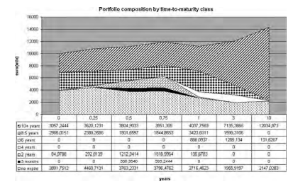
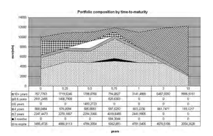
The optimal ALM strategy in the model depends on an extended set of asset and liability processes. We assume a multivariate normal distribution for monthly price returns of a representative set of market benchmarks including fixed income, equity, and real estate indices. The following $I=12$ investment opportunities are considered: for $i=1$ : the EURIBOR 3 months; for $i=2,3,4,5$, 6: the Barclays Treasury indices for maturity buckets $1-3,3-5,5-7,7-10$, and $10+$ years, respectively; for $i=7,8,9,10$ : the Barclays Corporate indices, again spanning maturities $1-3,3-5,5-7$, and $7-10$ years; finally for $i=11$ : the GPR Real Estate Europe index and $i=12$ : the MSCI EMU equity index. Recall that in our notation $I_{1}$ includes all fixed income assets and $I_{2}$ the real estate and equity investments.
The benchmarks represent total return indices incorporating over time the securities’ cash payments. In the definition of the strategic asset allocation problem, unlike
5 Dynamic Portfolio Management for Property and Casualty Insuranee
109
real estate and equity investments, money market and fixed income benchmarks are assumed to have a fixed maturity equal to their average duration ( 3 months, 2 years, 4,6 , and $8.5$ years for the corresponding Treasury and Corporate indices and 12 years for the $10+$ Treasury index). Income cashflows due to coupon payments will be estimated ex post through an approximation described below upon selling or expiry of fixed income benchmarks and disentangled from price returns. Equity investments will instead generate annual dividends through a price-adjusted random dividend yield. Finally, for real estate investments a simple model focusing only on price returns is considered. Scenario generation translates the indices return trajectories for the above market benchmarks into a tree process (see, for instance, the tree structure in Fig. 5.3) for the ALM coefficients (Consigli et al., 2010; Chapters 15 and 16 ): this is referred to in the sequel as the tree coefficient process. We rely on the process nodal realizations (Chapter 4 ) to identify the coefficients to be associated with each decision variable in the ALM model. We distinguish in the decision model between asset and liability coefficients.
统计代写|金融中的随机方法作业代写Stochastic Methods in Finance代考|Asset Return Scenarios
The following random coefficients must be derived from the data process simulations along the specified scenario tree. For each scenario $s$, at $t=t_{0}, t_{1}, \ldots, t_{n}=H$, we define
$\rho_{i, t}(s)$ : the return of asset $i$ at time $t$ in scenario $s$;
$\delta_{i, t}(s)$ : the dividend yield of asset $i$ at time $t$ in scenario $s$;
$\eta_{i, h, t}(s)$ : a positive interest at time $t$ in scenario $s$ per unit investment in asset $i \in I_{1}$, in epoch $h$;
$\gamma_{i, h, t}(s)$ : the capital gain at time $t$ in scenario $s$ per unit investment in asset $i \in I_{2}$ in epoch $h$;
$\zeta_{t}^{+/-}(s):$ the (positive and negative) interest rates on the cash account at time $t$ in scenario $s$.
Price refurns $\rho_{i, t}(s)$ under scenario s are directly computed from the associated benchmarks $V_{i, t}(s)$ assuming a multivariate normal distribution, with $\rho:=$ $\left{\rho_{i}(\omega)\right}, \rho \sim N(\mu, \Sigma)$, where $\omega$ denotes a generic random element, and $\mu$ and $\Sigma$ denote the return mean vector and variance-covariance matrix, respectively. In the statistical model we consider for $i \in I 12$ investment opportunities and the inflation rate. Denoting by $\Delta t$ a monthly time increment and given the initial values $V_{i, 0}$ for $i=1,2, \ldots, 12$, we assume a stochastic difference equation for $V_{i, t}:$
$$
\begin{aligned}
\rho_{i, t}(s) &=\frac{V_{i, t}(s)-V_{i, t-\Delta t}(s)}{V_{i, t}-\Delta t(s)}, \
\frac{\Delta V_{i, t}(s)}{V_{i, t}(s)}=\mu \Delta t+\Sigma \Delta W_{t}(s) .
\end{aligned}
$$
In $(5.12), \Delta W_{t} \sim N(0, \Delta t)$. We show in Tables $5.2$ and $5.3$ the estimated statistical parameters adopted to generate through Monte Carlo simulation (Consigli et al., 2010 ; Glasserman, 2003 ) the correlated monthly returns in (5.12) for each benchmark $i$ and scenario $s$. Monthly returns are then compounded according to the horizon partition (see Fig. 5.1) following a prespecified scenario tree structure. The return scenarios in tree form are then passed on to an algebraic language deterministic model generator to produce the stochastic program deterministic equivalent instance (Consigli and Dempster, 1998).
Equity dividends are determined independently in terms of the equity position at the beginning of a stage as $\sum_{i \in l_{2}} x_{i, f_{j-1}}(s) \delta_{i, t_{j}}(s)$, where $\delta_{i, t_{j}}(s) \sim N(0.02,0.005)$ is the dividend yield.
Interest margin $M_{t_{j}}(s)=I_{t_{j}}^{+}(s)-I_{t_{j}}^{-}(s)$ is computed by subtracting negative from positive interest cash flows. Negative interest $I_{t_{j}}^{-}(s)=z_{t_{j-1}}^{-}(s) \zeta_{t_{j}}^{-}(s)$ is generated by short positions on the current account according to a fixed $2 \%$ spread over the Euribor 3 -month rate for the current period. The positive interest rate for cash surplus is fixed at $\zeta^{+}(t, s)=0.5 \%$ for all $t$ and $s$.
Positive interest $I_{t_{j}}^{+}(s)$ is calculated from return scenarios of fixed income investments $i \in I_{2}$ using buying-selling price differences assuming initial unit investments; this may be regarded as a suitable first approximation. In the case of negative price differences, the loss is entirely attributed to price movements and the interest accrual is set to 0 .
We recognize that this is a significant simplifying assumption. It is adopted here to avoid the need for an explicit yield curve model, whose introduction would go beyond the scope of a case study. Nevertheless we believe that this simplification allows one to recognize the advantages of a dynamic version of the portfolio management problem.
统计代写|金融中的随机方法作业代写Stochastic Methods in Finance代考|Liability Scenarios
Annual premium renewals by P\&C policyholders represent the key technical income on which the company relies for its ongoing business requirements. Premiums have associated random insurance claims over the years and, depending on the business cycle and the claim class, they might induce different reserve requirements. The latter constitute the insurance company’s most relevant liability. In our analysis premiums are assumed to be written annually and will be stationary over the 10-year horizon with limited volatility. Insurance claims are also assumed to remain stable over time in nominal terms, but with an inflation adjustment that in the long term may affect the company’s short-term liquidity. For a given estimate of insurance premiums $R_{0}$ collected in the first year, along scenario $s$, for $t=t_{1}, t_{2}, \ldots, H$, with $e_{r} \sim N(1,0.03)$, we assume that
$$
R_{t j}(s)=\left[R_{t j-1}(s) \cdot e_{r}\right] .
$$
Insurance claims are assumed to grow annually at the inflation rate and in nominal terms are constant in expectation. For given initial liability $L_{0}$, with $e_{l} \sim$ $N(1,0.01)$
$$
L_{t_{j}}(s)=\left(L_{t_{j-1}}(s) \cdot e t\right)\left(1+\pi_{t_{j}}(s)\right) .
$$
Every year the liability stream is assumed to vary in the following year according to a normal distribution with the previous year’s mean and a $1 \%$ volatility per year with a further inflation adjustment. Given $\pi(0)$ at time 0 , the inflation process $\pi_{t}(s)$ is assumed to follow a mean-reverting process
$$
\Delta \pi_{t}(s)=\alpha_{\pi}\left(\mu-\pi_{t}(s)\right) \Delta t+\sigma_{\pi} \Delta W_{t}(s)
$$
with $\mu$ set in our case study to the $2 \%$ European central bank target and $\Delta W_{t} \cdots$ $N(0, \Delta t)$. As for the other liability variables technical resenves are computed as a linear function of the current liability as $\Lambda_{t}(s)=L_{t}(s) \cdot \lambda$, where $\lambda$ in our case study is approximated by $1 / 0.3$ as estimated by practitioner opinion.
Operational costs $C_{t_{j}}(s)$ include staff and back-office and are assumed to increase at the inflation rate. For a given initial estimate $C_{0}$, along each scenario and stage, we have
$$
C_{t_{j}}(s)=C_{t_{j-1}}(s) \cdot\left(1+\pi_{t_{j}}(s)\right)
$$
Bad liability scenarios will be induced by years of premium reductions associated with unexpected insurance claim increases, leading to higher reserve requirements that, in turn, would require a higher capital base. A stressed situation is discussed in Section $5.4$ to emphasize the flexibility of dynamic strategies to adapt to bad technical scenarios and compensate for such losses. The application also shows that within a dynamic framework the insurance manager is able to achieve an optimal trade-off between investment and technical profit generation across scenarios and over time, and between risky and less risky portfolio positions.
金融中的随机方法代写
统计代写|金融中的随机方法作业代写Stochastic Methods in Finance代考|Scenario Generation
模型中的最优 ALM 策略取决于一组扩展的资产和负债流程。我们假设一组具有代表性的市场基准(包括固定收益、股票和房地产指数)的月价格回报呈多元正态分布。以下一世=12考虑投资机会:一世=1: EURIBOR 3 个月; 为了一世=2,3,4,5, 6: 到期桶的巴克莱国库指数1−3,3−5,5−7,7−10, 和10+年,分别;为了一世=7,8,9,10:巴克莱公司指数,再次跨越期限1−3,3−5,5−7, 和7−10年; 终于为一世=11:GPR 房地产欧洲指数和一世=12: MSCI EMU 股票指数。回想一下,在我们的符号中一世1包括所有固定收益资产和一世2房地产和股权投资。
基准代表总回报指数,包括随着时间的推移证券的现金支付。在战略资产配置问题的定义中,与
5 财产险和意外险的动态投资组合管理
109
房地产和股权投资不同,假设货币市场和固定收益基准的固定期限等于它们的平均久期(3 个月,2年,4,6 和8.5相应的国库券和公司指数为 12 年,10+国库指数)。因支付息票而产生的收入现金流量将通过以下在固定收益基准出售或到期时描述的近似值进行事后估计,并与价格回报脱钩。相反,股权投资将通过价格调整后的随机股息收益率产生年度股息。最后,对于房地产投资,我们考虑了一个只关注价格回报的简单模型。情景生成将上述市场基准的指数回报轨迹转换为 ALM 系数的树形过程(例如,参见图 5.3 中的树形结构)(Consigli 等人,2010;第 15 章和第 16 章):这是后面称为树系数过程。我们依靠过程节点实现(第 4 章)来识别与 ALM 模型中的每个决策变量相关联的系数。我们在决策模型中区分资产和负债系数。
统计代写|金融中的随机方法作业代写Stochastic Methods in Finance代考|Asset Return Scenarios
以下随机系数必须从沿指定场景树的数据过程模拟中得出。对于每个场景s, 在吨=吨0,吨1,…,吨n=H,我们定义
ρ一世,吨(s): 资产回报一世有时吨在情景中s;
d一世,吨(s): 资产的股息收益率一世有时吨在情景中s;
这一世,H,吨(s): 对时间的积极兴趣吨在情景中s单位资产投资一世∈一世1, 在纪元H;
C一世,H,吨(s):当时的资本收益吨在情景中s单位资产投资一世∈一世2在时代H;
G吨+/−(s):现金账户当时的(正和负)利率吨在情景中s.
价格返还ρ一世,吨(s)场景下的 s 直接从相关的基准计算五一世,吨(s)假设一个多元正态分布,ρ:= \left{\rho_{i}(\omega)\right}, \rho \sim N(\mu, \Sigma)\left{\rho_{i}(\omega)\right}, \rho \sim N(\mu, \Sigma), 在哪里ω表示一个通用随机元素,并且μ和Σ分别表示返回均值向量和方差-协方差矩阵。在我们考虑的统计模型中一世∈一世12投资机会和通货膨胀率。表示Δ吨每月时间增量并给定初始值五一世,0为了一世=1,2,…,12,我们假设一个随机差分方程五一世,吨:
ρ一世,吨(s)=五一世,吨(s)−五一世,吨−Δ吨(s)五一世,吨−Δ吨(s), Δ五一世,吨(s)五一世,吨(s)=μΔ吨+ΣΔ在吨(s).
在(5.12),Δ在吨∼ñ(0,Δ吨). 我们在表格中显示5.2和5.3通过蒙特卡罗模拟(Consigli 等人,2010 年;Glasserman,2003 年)生成的估计统计参数 每个基准在 (5.12) 中的相关月收益一世和场景s. 然后按照预先指定的情景树结构,根据水平分区(见图 5.1)对月回报进行复合。然后将树形式的返回场景传递给代数语言确定性模型生成器,以生成随机程序确定性等效实例(Consigli 和 Dempster,1998 年)。
股权分红根据阶段开始时的股权状况独立确定∑一世∈一世2X一世,Fj−1(s)d一世,吨j(s), 在哪里d一世,吨j(s)∼ñ(0.02,0.005)是股息收益率。
息差米吨j(s)=一世吨j+(s)−一世吨j−(s)通过从正利息现金流中减去负数来计算。负利率一世吨j−(s)=和吨j−1−(s)G吨j−(s)是由经常账户的空头头寸根据固定的2%分布在当前期间的 3 个月 Euribor 利率上。现金盈余的正利率固定为G+(吨,s)=0.5%对全部吨和s.
积极的兴趣一世吨j+(s)根据固定收益投资的回报方案计算一世∈一世2假设初始单位投资,使用买卖价格差异;这可以被认为是一个合适的第一近似值。在负价格差异的情况下,损失完全归因于价格变动,应计利息设置为 0。
我们认识到这是一个重要的简化假设。这里采用它是为了避免需要明确的收益率曲线模型,其引入将超出案例研究的范围。尽管如此,我们相信这种简化可以让人们认识到动态版本的投资组合管理问题的优势。
统计代写|金融中的随机方法作业代写Stochastic Methods in Finance代考|Liability Scenarios
财产险保单持有人的年度保费续保代表了公司依赖其持续业务需求的关键技术收入。多年来,保费与随机保险索赔相关,并且根据商业周期和索赔类别,它们可能会导致不同的准备金要求。后者构成保险公司最相关的责任。在我们的分析中,假设保费为每年一次,并且在 10 年内保持稳定,波动性有限。保险索赔也被假设在名义上随着时间的推移保持稳定,但通货膨胀调整从长远来看可能会影响公司的短期流动性。对于给定的保险费估计R0第一年收集,沿情景s, 为了吨=吨1,吨2,…,H, 和和r∼ñ(1,0.03), 我们假设
R吨j(s)=[R吨j−1(s)⋅和r].
假设保险索赔每年以通货膨胀率增长,并且名义上的预期是不变的。对于给定的初始责任大号0, 和和一世∼ ñ(1,0.01)
大号吨j(s)=(大号吨j−1(s)⋅和吨)(1+圆周率吨j(s)).
假设每年的负债流在下一年按照正态分布变化,上一年的平均值和1%随着通货膨胀的进一步调整,每年波动。给定圆周率(0)在时间 0 ,膨胀过程圆周率吨(s)假设遵循均值回复过程Δ圆周率吨(s)=一种圆周率(μ−圆周率吨(s))Δ吨+σ圆周率Δ在吨(s)
和μ在我们的案例研究中设置为2%欧洲央行目标和Δ在吨⋯ ñ(0,Δ吨). 至于其他负债变量,技术收益被计算为当前负债的线性函数Λ吨(s)=大号吨(s)⋅λ, 在哪里λ在我们的案例研究中,近似于1/0.3根据从业者的意见估计。
运营成本C吨j(s)包括员工和后台,并假设随着通货膨胀率增加。对于给定的初始估计C0,在每个场景和阶段,我们有
C吨j(s)=C吨j−1(s)⋅(1+圆周率吨j(s))
与意外保险索赔增加相关的多年保费减少将引发不良责任情景,从而导致更高的准备金要求,进而需要更高的资本基础。第一部分讨论了压力情况5.4强调动态策略的灵活性,以适应糟糕的技术情景并弥补此类损失。该应用程序还表明,在动态框架内,保险经理能够在不同场景和一段时间内以及在风险和风险较低的投资组合头寸之间实现投资和技术利润产生之间的最佳权衡。

统计代写请认准statistics-lab™. statistics-lab™为您的留学生涯保驾护航。统计代写|python代写代考
随机过程代考
在概率论概念中,随机过程是随机变量的集合。 若一随机系统的样本点是随机函数,则称此函数为样本函数,这一随机系统全部样本函数的集合是一个随机过程。 实际应用中,样本函数的一般定义在时间域或者空间域。 随机过程的实例如股票和汇率的波动、语音信号、视频信号、体温的变化,随机运动如布朗运动、随机徘徊等等。
贝叶斯方法代考
贝叶斯统计概念及数据分析表示使用概率陈述回答有关未知参数的研究问题以及统计范式。后验分布包括关于参数的先验分布,和基于观测数据提供关于参数的信息似然模型。根据选择的先验分布和似然模型,后验分布可以解析或近似,例如,马尔科夫链蒙特卡罗 (MCMC) 方法之一。贝叶斯统计概念及数据分析使用后验分布来形成模型参数的各种摘要,包括点估计,如后验平均值、中位数、百分位数和称为可信区间的区间估计。此外,所有关于模型参数的统计检验都可以表示为基于估计后验分布的概率报表。
广义线性模型代考
广义线性模型(GLM)归属统计学领域,是一种应用灵活的线性回归模型。该模型允许因变量的偏差分布有除了正态分布之外的其它分布。
statistics-lab作为专业的留学生服务机构,多年来已为美国、英国、加拿大、澳洲等留学热门地的学生提供专业的学术服务,包括但不限于Essay代写,Assignment代写,Dissertation代写,Report代写,小组作业代写,Proposal代写,Paper代写,Presentation代写,计算机作业代写,论文修改和润色,网课代做,exam代考等等。写作范围涵盖高中,本科,研究生等海外留学全阶段,辐射金融,经济学,会计学,审计学,管理学等全球99%专业科目。写作团队既有专业英语母语作者,也有海外名校硕博留学生,每位写作老师都拥有过硬的语言能力,专业的学科背景和学术写作经验。我们承诺100%原创,100%专业,100%准时,100%满意。
机器学习代写
随着AI的大潮到来,Machine Learning逐渐成为一个新的学习热点。同时与传统CS相比,Machine Learning在其他领域也有着广泛的应用,因此这门学科成为不仅折磨CS专业同学的“小恶魔”,也是折磨生物、化学、统计等其他学科留学生的“大魔王”。学习Machine learning的一大绊脚石在于使用语言众多,跨学科范围广,所以学习起来尤其困难。但是不管你在学习Machine Learning时遇到任何难题,StudyGate专业导师团队都能为你轻松解决。
多元统计分析代考
基础数据: $N$ 个样本, $P$ 个变量数的单样本,组成的横列的数据表
变量定性: 分类和顺序;变量定量:数值
数学公式的角度分为: 因变量与自变量
时间序列分析代写
随机过程,是依赖于参数的一组随机变量的全体,参数通常是时间。 随机变量是随机现象的数量表现,其时间序列是一组按照时间发生先后顺序进行排列的数据点序列。通常一组时间序列的时间间隔为一恒定值(如1秒,5分钟,12小时,7天,1年),因此时间序列可以作为离散时间数据进行分析处理。研究时间序列数据的意义在于现实中,往往需要研究某个事物其随时间发展变化的规律。这就需要通过研究该事物过去发展的历史记录,以得到其自身发展的规律。
回归分析代写
多元回归分析渐进(Multiple Regression Analysis Asymptotics)属于计量经济学领域,主要是一种数学上的统计分析方法,可以分析复杂情况下各影响因素的数学关系,在自然科学、社会和经济学等多个领域内应用广泛。
MATLAB代写
MATLAB 是一种用于技术计算的高性能语言。它将计算、可视化和编程集成在一个易于使用的环境中,其中问题和解决方案以熟悉的数学符号表示。典型用途包括:数学和计算算法开发建模、仿真和原型制作数据分析、探索和可视化科学和工程图形应用程序开发,包括图形用户界面构建MATLAB 是一个交互式系统,其基本数据元素是一个不需要维度的数组。这使您可以解决许多技术计算问题,尤其是那些具有矩阵和向量公式的问题,而只需用 C 或 Fortran 等标量非交互式语言编写程序所需的时间的一小部分。MATLAB 名称代表矩阵实验室。MATLAB 最初的编写目的是提供对由 LINPACK 和 EISPACK 项目开发的矩阵软件的轻松访问,这两个项目共同代表了矩阵计算软件的最新技术。MATLAB 经过多年的发展,得到了许多用户的投入。在大学环境中,它是数学、工程和科学入门和高级课程的标准教学工具。在工业领域,MATLAB 是高效研究、开发和分析的首选工具。MATLAB 具有一系列称为工具箱的特定于应用程序的解决方案。对于大多数 MATLAB 用户来说非常重要,工具箱允许您学习和应用专业技术。工具箱是 MATLAB 函数(M 文件)的综合集合,可扩展 MATLAB 环境以解决特定类别的问题。可用工具箱的领域包括信号处理、控制系统、神经网络、模糊逻辑、小波、仿真等。