标签: MATH 866

统计代写|金融中的随机方法作业代写Stochastic Methods in Finance代考| Pricing Coupon-Bearing Bonds

如果你也在 怎样代写金融中的随机方法Stochastic Methods in Finance这个学科遇到相关的难题,请随时右上角联系我们的24/7代写客服。

随机建模是金融模型的一种形式,用于帮助做出投资决策。这种类型的模型使用随机变量预测不同条件下各种结果的概率。随着现代经济学、金融学实证研究的发展金融中的随机方法Stochastic Methods in Finance作为一种数学工具具有越来越重要的应用价值

statistics-lab™ 为您的留学生涯保驾护航 在代写金融中的随机方法Stochastic Methods in Finance方面已经树立了自己的口碑, 保证靠谱, 高质且原创的统计Statistics代写服务。我们的专家在代写金融中的随机方法Stochastic Methods in Finance方面经验极为丰富,各种代写金融中的随机方法Stochastic Methods in Finance相关的作业也就用不着说。

我们提供的金融中的随机方法Stochastic Methods in Finance及其相关学科的代写,服务范围广, 其中包括但不限于:

  • Statistical Inference 统计推断
  • Statistical Computing 统计计算
  • Advanced Probability Theory 高等楖率论
  • Advanced Mathematical Statistics 高等数理统计学
  • (Generalized) Linear Models 广义线性模型
  • Statistical Machine Learning 统计机器学习
  • Longitudinal Data Analysis 纵向数据分析
  • Foundations of Data Science 数据科学基础
统计代写|金融中的随机方法作业代写Stochastic Methods in Finance代考| Pricing Coupon-Bearing Bonds

统计代写|金融中的随机方法作业代写Stochastic Methods in Finance代考|Pricing Coupon-Bearing Bonds

As sufficient historical data on Euro coupon-bearing Treasury bonds is difficult to obtain we use the zero-coupon yield curve to construct the relevant bonds. Coupons on newly-issued bonds are generally closely related to the corresponding spot rate at the time, so the current zero-coupon yield with maturity $T$ is used as a proxy for the coupon rate of a coupon-bearing Treasury bond with maturity $T$. For example, on scenario $\omega$ the coupon rate $\delta_{2}^{B^{10}}(\omega)$ on a newly issued 10-year Treasury bond at time $t=2$ will be set equal to the projected 10 -year spot rate $y_{2,10}(\omega)$ at time $t=2$.
Generally
$$
\begin{array}{llr}
\delta_{t}^{B^{(T)}}(\omega)=y_{t, T}(\omega) & \forall t \in T^{d} & \forall \omega \in \Omega \
\delta_{t}^{B^{(T)}}(\omega)=\delta_{\lfloor t\rfloor}^{(T)}(\omega) & \forall t \in T^{i} & \forall \omega \in \Omega,
\end{array}
$$
where L.」 denotes integral part. This ensures that as the yield curve falls, coupons on newly-issued bonds will go down correspondingly and each coupon cash flow will be discounted at the appropriate zero-coupon yield.

The bonds are assumed to pay coupons semi-annually. Since we roll the bonds on an annual basis, a coupon will be received after six months and again after a year just before the bond is sold. This forces us to distinguish between the price at which the bond is sold at rebalancing times and the price at which the new bond is purchased.

Let $P_{t, B^{(T)}}^{(\text {sell }}$ denote the selling price of the bond $B^{(T)}$ at time $t$, assuming two coupons have now been paid out and the time to maturity is equal to $T-1$, and let $P_{t, B^{(t)}}^{(\text {tuy })}$ denote the price of a newly issued coupon-bearing Treasury bond with a maturity equal to $T$.
The “buy’ bond price at time $t$ is given by
$$
\begin{aligned}
B_{t}^{T}(\omega)=& F^{B^{T}} e^{-(T+\lfloor t]-t) y_{t, T+\lfloor t \mid-t}(\omega)} \
&+\sum_{s=\frac{|2|}{2}+\frac{1}{2}, \frac{\lfloor 2\rfloor \mid}{2}+1, \ldots,[t]+T} \frac{\delta^{A^{T}}(\omega)}{2} F^{B^{T}} e^{-(s-t) y_{t, t x-t)}(\omega)}
\end{aligned}
$$
where the principal of the bond is discounted in the first term and the stream of coupon payments in the second.
At rebalancing times $t$ the sell price of the bond is given by
$$
B_{t}^{T}(\omega)=F^{B^{T}} e^{-(T-1) y_{i, T-1}(\omega)}+\sum_{s=\frac{1}{2}, 1, \ldots, T-1} \frac{\delta_{i-1}^{B^{T}}(\omega)}{2} F^{B^{T}} e^{-(s-t) y,(\omega-t)(\omega)}
$$
$\omega \in \Omega \quad t \in\left{T^{d} \backslash{0}\right} \cup{T}$with coupon rate $\delta_{t-1}^{B^{T}}(\omega)$. The coupon rate is then reset for the newly-issued Treasury bond of the same maturity. We assume that the coupons paid at six months are re-invested in the off-the-run bonds. This gives the following adjustment to the amount held in bond $B^{T}$ at time $t$

统计代写|金融中的随机方法作业代写Stochastic Methods in Finance代考|Historical Backtests

We will look at an historical backtest in which statistical models are fitted to data up to a trading time $t$ and scenario trees are generated to some chosen horizon $t+T$. The optimal root node decisions are then implemented at time $t$ and compared to the historical returns at time $t+1$. Afterwards the whole procedure is rolled forward for T trading times.
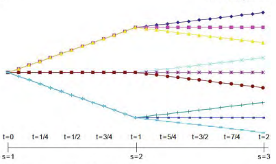
Our backtest will involve a telescoping horizon as depicted in Figure $4 .$
At each decision time $t$ the parameters of the stochastic processes driving the stock return and the three factors of the term structure model are re-calibrated using historical data up to and including time $t$ and the initial values of the simulated scenarios are given by the actual historical values of the variables at these times. Re-calibrating the simulator parameters at each successive initial decision time $t$ captures information in the history of the variables up to that point.

Although the optimal second and later-stage decisions of a given problem may be of “what-if” interest, manager and decision maker focus is on the implementable first-stage decisions which are hedged against the simnlated future uncertainties The reasons for implementing stochastic optimization programmes in this way are twofold. Firstly, after one year has passed the actual values of the variables realized may not coincide with any of the values of the variables in the simulated scenarios. In this case the optimal investment policy would be undefined, as the model only has

optimal decisions defined for the nodes on the simulated scenarios. Secondly, as one more year has passed new information has become available to re-calibrate the simulator’s parameters. Relying on the original optimal investment strategies will ignore this information. For more on backtesting procedures for stochastic optimization models see Dempster et al. (2003).

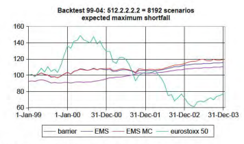
For our backtests we will use three different tree structures with approximately the same number of scenarios, but with an increasing initial branching factor. We first solve the five-year problem using a $6.6 .6 .6 .6$ tree, which gives 7776 scenarios. Then we use $32.4 .4 .4 .4=8192$ scenarios and finally the extreme case of $512.2 .2 .2 .2=8192$ scenarios.

统计代写|金融中的随机方法作业代写Stochastic Methods in Finance代考|Robustness of Backtest Results

Empirical equity returns are now well known not to be normally distributed but rather to exhibit complex behaviour including fat tails. To investigate how the EMS MC model performs with more realistic asset return distributions we report in this section experiments using a geometric Brownian motion with Poisson jumps to model equity returns. The stock price process $\mathbf{S}$ is now assumed to follow
$$
\frac{d \mathbf{S}{t}}{\mathbf{S}{t}}=\bar{\mu}{S} d t+\tilde{\sigma}{S} d \overline{\mathbf{W}}{t}^{S}+\mathbf{J}{t} d \mathbf{N}_{t}
$$
where $\mathbf{N}$ is an independent Poisson process with intensity $\lambda$ and the jump saltus $\mathbf{J}$ at Poisson epochs is a normal random variable.

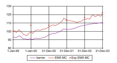
As the EMS MC model and the $512.2 .2 .2 .2$ tree provided the best results with Gaussian returns the backtest is repeated for this model and treesize. Figure 12 gives the historical backtest results and Tables 5 and 6 represent the allocations for the $512.2 .2 .2 .2$ tests with the EMS MC model for the original GBM process and the GBM with Poisson jumps process respectively. The main difference in the two tables is that the investment in equity is substantially lower initially when the equity index volatility is high (going down to $0.1 \%$ when the volatility is $28 \%$ in 2001 ), but then increases as the volatility comes down to $23 \%$ in 2003 . This is born out by Figure 12 which shows much more realistic in-sample one-year-ahead portfolio wealth predictions (cf. Figure 10$)$ and a 140 basis point increase in terminal historical fund return over the Gaussian model. These phenomena are the result of the calibration of the normal jump saltus distributions to have negative means and hence more downward than upwards jumps resulting in downwardly skewed equity index return distributions, but with the same compensated drift as in the GBM case.

统计代写|金融中的随机方法作业代写Stochastic Methods in Finance代考| Pricing Coupon-Bearing Bonds

金融中的随机方法代写

统计代写|金融中的随机方法作业代写Stochastic Methods in Finance代考|Pricing Coupon-Bearing Bonds

由于难以获得足够的欧元附息国债的历史数据,我们使用零息票收益率曲线来构建相关债券。新发行债券的票面利率一般与当时对应的即期利率密切相关,因此当前的零票面收益率与到期吨用于代表有息票到期的国债的票面利率吨. 例如,在场景ω票面利率d2乙10(ω)当时新发行的 10 年期国债吨=2将设定为等于预计的 10 年期即期汇率是2,10(ω)有时吨=2.
一般来说
d吨乙(吨)(ω)=是吨,吨(ω)∀吨∈吨d∀ω∈Ω d吨乙(吨)(ω)=d⌊吨⌋(吨)(ω)∀吨∈吨一世∀ω∈Ω,
其中L.”表示整数部分。这确保了随着收益率曲线的下降,新发行债券的票面利率将相应下降,每笔票面现金流量将以适当的零票面收益率贴现。

假设债券每半年支付一次息票。由于我们每年滚动债券,因此将在六个月后收到息票,并在债券出售前一年再次收到票息。这迫使我们区分在再平衡时出售债券的价格和购买新债券的价格。

让磷吨,乙(吨)(卖 表示债券的售价乙(吨)有时吨,假设现在已经支付了两张息票并且到期时间等于吨−1, 然后让磷吨,乙(吨)(虽然 )表示新发行的附息国债的价格,期限等于吨.
当时的“买入”债券价格吨是(谁)给的
乙吨吨(ω)=F乙吨和−(吨+⌊吨]−吨)是吨,吨+⌊吨∣−吨(ω) +∑s=|2|2+12,⌊2⌋∣2+1,…,[吨]+吨d一种吨(ω)2F乙吨和−(s−吨)是吨,吨X−吨)(ω)
其中债券的本金在第一期贴现,在第二期贴现付息流。
在再平衡时吨债券的售价由下式给出
乙吨吨(ω)=F乙吨和−(吨−1)是一世,吨−1(ω)+∑s=12,1,…,吨−1d一世−1乙吨(ω)2F乙吨和−(s−吨)是,(ω−吨)(ω)
\omega \in \Omega \quad t \in\left{T^{d} \反斜杠{0}\right} \cup{T}\omega \in \Omega \quad t \in\left{T^{d} \反斜杠{0}\right} \cup{T}以票面利率d吨−1乙吨(ω). 然后为新发行的相同期限的国债重置票面利率。我们假设在六个月内支付的息票被重新投资于期外债券。这对持有的债券金额进行了以下调整乙吨有时吨

统计代写|金融中的随机方法作业代写Stochastic Methods in Finance代考|Historical Backtests

我们将看一个历史回测,其中统计模型适合交易时间的数据吨和场景树生成到一些选定的地平线吨+吨. 然后及时实施最佳根节点决策吨并与当时的历史回报率相比吨+1. 之后,整个过程向前滚动 T 个交易时间。
我们的回测将涉及如图所示的伸缩视野4.
在每个决策时间吨驱动股票收益的随机过程参数和期限结构模型的三个因素使用历史数据重新校准,包括时间吨模拟场景的初始值由这些时间变量的实际历史值给出。在每个连续的初始决策时间重新校准模拟器参数吨捕获该点之前的变量历史信息。

尽管给定问题的最佳第二阶段和后期决策可能具有“假设”的兴趣,但经理和决策者的重点是可实施的第一阶段决策,这些决策可以对冲模拟的未来不确定性 实施随机优化的原因这种方式的程序是双重的。首先,在一年过去之后,实际变量的实际值可能与模拟场景中的任何变量值不一致。在这种情况下,最优投资政策将是不确定的,因为模型只有

为模拟场景中的节点定义的最佳决策。其次,随着一年又过去了,新信息可用于重新校准模拟器的参数。依靠原来的最优投资策略会忽略这些信息。有关随机优化模型的回测程序的更多信息,请参阅 Dempster 等人。(2003 年)。

对于我们的回测,我们将使用三种不同的树结构,它们的场景数量大致相同,但初始分支因子会增加。我们首先使用一个解决五年问题6.6.6.6.6树,它给出了 7776 个场景。然后我们使用32.4.4.4.4=8192场景,最后是极端情况512.2.2.2.2=8192情景。

统计代写|金融中的随机方法作业代写Stochastic Methods in Finance代考|Robustness of Backtest Results

现在众所周知,经验股票收益不是正态分布的,而是表现出复杂的行为,包括肥尾。为了研究 EMS MC 模型如何在更现实的资产回报分布中执行,我们在本节中报告了使用具有泊松跳跃的几何布朗运动来模拟股票回报的实验。股价过程小号现在假设遵循
d小号吨小号吨=μ¯小号d吨+σ~小号d在¯吨小号+Ĵ吨dñ吨
在哪里ñ是具有强度的独立泊松过程λ和跳跃的盐Ĵ在 Poisson epochs 是一个正态随机变量。

作为 EMS MC 模型和512.2.2.2.2树提供了高斯返回的最佳结果,为此模型和树大小重复回测。图 12 给出了历史回测结果,表 5 和表 6 代表了512.2.2.2.2分别使用 EMS MC 模型对原始 GBM 过程和具有泊松跳跃过程的 GBM 进行测试。两个表的主要区别在于,当股票指数波动性较高时(下降至0.1%当波动率为28%2001 年),但随着波动性下降至23%2003 年。图 12 证明了这一点,该图显示了样本内未来一年投资组合财富预测更为现实(参见图 10)与高斯模型相比,最终历史基金回报增加了 140 个基点。这些现象是正态跳跃盐度分布校准为负均值的结果,因此向下跳跃多于向上跳跃,导致股指收益分布向下倾斜,但补偿漂移与 GBM 情况相同。

统计代写|金融中的随机方法作业代写Stochastic Methods in Finance代考 请认准statistics-lab™

统计代写请认准statistics-lab™. statistics-lab™为您的留学生涯保驾护航。统计代写|python代写代考

随机过程代考

在概率论概念中,随机过程随机变量的集合。 若一随机系统的样本点是随机函数,则称此函数为样本函数,这一随机系统全部样本函数的集合是一个随机过程。 实际应用中,样本函数的一般定义在时间域或者空间域。 随机过程的实例如股票和汇率的波动、语音信号、视频信号、体温的变化,随机运动如布朗运动、随机徘徊等等。

贝叶斯方法代考

贝叶斯统计概念及数据分析表示使用概率陈述回答有关未知参数的研究问题以及统计范式。后验分布包括关于参数的先验分布,和基于观测数据提供关于参数的信息似然模型。根据选择的先验分布和似然模型,后验分布可以解析或近似,例如,马尔科夫链蒙特卡罗 (MCMC) 方法之一。贝叶斯统计概念及数据分析使用后验分布来形成模型参数的各种摘要,包括点估计,如后验平均值、中位数、百分位数和称为可信区间的区间估计。此外,所有关于模型参数的统计检验都可以表示为基于估计后验分布的概率报表。

广义线性模型代考

广义线性模型(GLM)归属统计学领域,是一种应用灵活的线性回归模型。该模型允许因变量的偏差分布有除了正态分布之外的其它分布。

statistics-lab作为专业的留学生服务机构,多年来已为美国、英国、加拿大、澳洲等留学热门地的学生提供专业的学术服务,包括但不限于Essay代写,Assignment代写,Dissertation代写,Report代写,小组作业代写,Proposal代写,Paper代写,Presentation代写,计算机作业代写,论文修改和润色,网课代做,exam代考等等。写作范围涵盖高中,本科,研究生等海外留学全阶段,辐射金融,经济学,会计学,审计学,管理学等全球99%专业科目。写作团队既有专业英语母语作者,也有海外名校硕博留学生,每位写作老师都拥有过硬的语言能力,专业的学科背景和学术写作经验。我们承诺100%原创,100%专业,100%准时,100%满意。

机器学习代写

随着AI的大潮到来,Machine Learning逐渐成为一个新的学习热点。同时与传统CS相比,Machine Learning在其他领域也有着广泛的应用,因此这门学科成为不仅折磨CS专业同学的“小恶魔”,也是折磨生物、化学、统计等其他学科留学生的“大魔王”。学习Machine learning的一大绊脚石在于使用语言众多,跨学科范围广,所以学习起来尤其困难。但是不管你在学习Machine Learning时遇到任何难题,StudyGate专业导师团队都能为你轻松解决。

多元统计分析代考


基础数据: $N$ 个样本, $P$ 个变量数的单样本,组成的横列的数据表
变量定性: 分类和顺序;变量定量:数值
数学公式的角度分为: 因变量与自变量

时间序列分析代写

随机过程,是依赖于参数的一组随机变量的全体,参数通常是时间。 随机变量是随机现象的数量表现,其时间序列是一组按照时间发生先后顺序进行排列的数据点序列。通常一组时间序列的时间间隔为一恒定值(如1秒,5分钟,12小时,7天,1年),因此时间序列可以作为离散时间数据进行分析处理。研究时间序列数据的意义在于现实中,往往需要研究某个事物其随时间发展变化的规律。这就需要通过研究该事物过去发展的历史记录,以得到其自身发展的规律。

回归分析代写

多元回归分析渐进(Multiple Regression Analysis Asymptotics)属于计量经济学领域,主要是一种数学上的统计分析方法,可以分析复杂情况下各影响因素的数学关系,在自然科学、社会和经济学等多个领域内应用广泛。

MATLAB代写

MATLAB 是一种用于技术计算的高性能语言。它将计算、可视化和编程集成在一个易于使用的环境中,其中问题和解决方案以熟悉的数学符号表示。典型用途包括:数学和计算算法开发建模、仿真和原型制作数据分析、探索和可视化科学和工程图形应用程序开发,包括图形用户界面构建MATLAB 是一个交互式系统,其基本数据元素是一个不需要维度的数组。这使您可以解决许多技术计算问题,尤其是那些具有矩阵和向量公式的问题,而只需用 C 或 Fortran 等标量非交互式语言编写程序所需的时间的一小部分。MATLAB 名称代表矩阵实验室。MATLAB 最初的编写目的是提供对由 LINPACK 和 EISPACK 项目开发的矩阵软件的轻松访问,这两个项目共同代表了矩阵计算软件的最新技术。MATLAB 经过多年的发展,得到了许多用户的投入。在大学环境中,它是数学、工程和科学入门和高级课程的标准教学工具。在工业领域,MATLAB 是高效研究、开发和分析的首选工具。MATLAB 具有一系列称为工具箱的特定于应用程序的解决方案。对于大多数 MATLAB 用户来说非常重要,工具箱允许您学习应用专业技术。工具箱是 MATLAB 函数(M 文件)的综合集合,可扩展 MATLAB 环境以解决特定类别的问题。可用工具箱的领域包括信号处理、控制系统、神经网络、模糊逻辑、小波、仿真等。

R语言代写问卷设计与分析代写
PYTHON代写回归分析与线性模型代写
MATLAB代写方差分析与试验设计代写
STATA代写机器学习/统计学习代写
SPSS代写计量经济学代写
EVIEWS代写时间序列分析代写
EXCEL代写深度学习代写
SQL代写各种数据建模与可视化代写

统计代写|金融中的随机方法作业代写Stochastic Methods in Finance代考| Objective Functions: Expected Average Shortfall

如果你也在 怎样代写金融中的随机方法Stochastic Methods in Finance这个学科遇到相关的难题,请随时右上角联系我们的24/7代写客服。

随机建模是金融模型的一种形式,用于帮助做出投资决策。这种类型的模型使用随机变量预测不同条件下各种结果的概率。随着现代经济学、金融学实证研究的发展金融中的随机方法Stochastic Methods in Finance作为一种数学工具具有越来越重要的应用价值

statistics-lab™ 为您的留学生涯保驾护航 在代写金融中的随机方法Stochastic Methods in Finance方面已经树立了自己的口碑, 保证靠谱, 高质且原创的统计Statistics代写服务。我们的专家在代写金融中的随机方法Stochastic Methods in Finance方面经验极为丰富,各种代写金融中的随机方法Stochastic Methods in Finance相关的作业也就用不着说。

我们提供的金融中的随机方法Stochastic Methods in Finance及其相关学科的代写,服务范围广, 其中包括但不限于:

  • Statistical Inference 统计推断
  • Statistical Computing 统计计算
  • Advanced Probability Theory 高等楖率论
  • Advanced Mathematical Statistics 高等数理统计学
  • (Generalized) Linear Models 广义线性模型
  • Statistical Machine Learning 统计机器学习
  • Longitudinal Data Analysis 纵向数据分析
  • Foundations of Data Science 数据科学基础
统计代写|金融中的随机方法作业代写Stochastic Methods in Finance代考| Objective Functions: Expected Average Shortfall

统计代写|金融中的随机方法作业代写Stochastic Methods in Finance代考|Expected Maximum Shortfall

Starting with an initial wealth $W_{0}$ and an annual nominal guarantee of $G$, the liability at the planning horizon at time $T$ is given by
$$
W_{0}(1+G)^{T}
$$
To price the liability at time $t<T$ consider a zero-coupon Treasury bond, which pays 1 at time $T$, 1.e. $L_{T}(\omega)=1$, tor all scenarıos $\omega \in \lesssim 2$. 1 he zero-coupon Treasury bond price at time $t$ in scenario $\omega$ assuming continuous compounding is given by
$$
Z_{t}(\omega)=e^{-y_{t, T}(\omega)(T-t)}
$$

where $y_{t, T}(\omega)$ is the zero-coupon Treasury yield with maturity $T$ at time $t$ in scenario $\omega$.

This gives a formula for the value of the nominal or fixed guarantee barrier at time $t$ in scenario $\omega$ as
$$
L_{t}^{N}(\omega):=W_{0}(1+G)^{T} Z_{t}(\omega)=W_{0}(1+G)^{T} e^{-y_{t} T(\omega)(T-t)}
$$
In a minimum guaranteed return fund the objective of the fund manager is twofold; firstly to manage the investment strategies of the fund and secondly to take into account the guarantees given to all investors. Investment strategies must ensure that the guarantee for all participants of the fund is met with a high probability.

In practice the guarantor (the parent bank of the fund manager) will ensure the investor guarantee is met by forcing the purchase of the zero coupon bond of (22) when the fund is sufficiently near the barrier defined by $(23)$. Since all upside potential to investors is thus foregone, the aim of the fund manager is to fall below the barrier with acceptably small if not zero probability.

Ideally we would add a constraint limiting the probability of falling below the barrier in a VaR-type minimum guarantee constraint, i.e.
$$
P\left(\max {t \in T \text { loal }} h{t}(\omega)>0\right) \leq \alpha
$$
for $\alpha$ small. However, such scenario-based probabilistic constraints are extremely difficult to implement, as they may without further assumptions convert the convex large-scale optimization problem into a non-convex one. We therefore use the following two convex approximations in which we trade off the risk of falling below the barrier against the return in the form of the expected sum of wealth.

Firstly, we look at the expected average shortfall (EAS) model in which the objective function is given by:
$\left{\max {\left{\begin{array}{l}x{t, a}(\omega), x_{t, \alpha}^{+}(\omega), x_{t, a}^{-}(\omega): \ a \in A, \omega \in \Omega, t \in T^{d} \cup[T]\end{array}\right.}\left{\sum_{\omega \in \Omega} \sum_{\left.t \in T^{d} \cup \mid T\right]} p(\omega)\left((1-\beta) W_{t}(\omega)-\beta \frac{h_{S}(\omega)}{\mid T^{d} \cup[T \mid}\right)\right}\right.$
$\left.-\beta\left(\sum_{\omega \in \Omega} p(\omega) \sum_{t \in T^{d} \cup{T]} \frac{h_{d}(\omega)}{\left|T^{w} \cup[T]\right|}\right)\right}$

统计代写|金融中的随机方法作业代写Stochastic Methods in Finance代考|Bond Pricing

In this section we present a three-factor term structure model which we will use to price both our bond portfolio and the fund’s liability. Many interest-rate models, like the classic one-factor Vasicek (1977) and Cox, Ingersoll, and Ross (1985) class of models and even more recent multi-factor models like Anderson and Lund (1997), concentrate on modeling just the short-term rate.

However for the minimum guaranteed retum funds we have to deal with a longterm liability and bonds of varying maturities. We therefore must capture the dynamics of the whole term structure. This has been achieved by using the economic factor model described below in Section 3.1. In Section $3.2$ we describe the pricing of coupon-bearing bonds and Section $3.3$ investigates the consequences of rolling the bonds on an annual basis.

统计代写|金融中的随机方法作业代写Stochastic Methods in Finance代考|Yield Curve Model

To capture the dynamics of the whole term structure, we will use a Gaussian economic factor model (EFM) (see Campbell $(2000)$ and also Nelson and Siegel (1987)) whose evolution under the risk-neutral measure $Q$ is determined by the stochastic differential equations
$$
\begin{aligned}
&\mathbf{d X} \mathbf{X}{t}=\left(\mu{X}-\lambda_{X} X_{t}\right) d t+\sigma_{X} \mathbf{d} \mathbf{W}{t}^{X} \ &\mathbf{d Y { t }}=\left(\mu_{Y}-\lambda_{Y} Y_{t}\right) d t+\sigma_{Y} \mathbf{d} \mathbf{W}{t}^{Y} \ &\mathbf{d R}{t}=k\left(X_{t}+Y_{t}-R_{t}\right) d t+\sigma_{R} \mathbf{d W}{t}^{R} \end{aligned} $$ where the $d W$ terms are correlated. The three unobservable Gaussian factors $\mathbf{R}, \mathbf{X}$ and $\mathbf{Y}$ represent respectively a short rate, a long rate and (minus) the slope between an instantaneous short rate and the long rate. Solving these equations the following formula for the yield at time $t$ with time to maturity equal to $T-t$ is obtained (for a derivation, see Medova et $a l ., 2005$ ) $$ y{t, T}=\frac{A(t, T) R_{t}+B(t, T) X_{t}+C(t, T) Y_{t}+D(t, T)}{T}
$$
where
$$
\begin{aligned}
&B(t, T):=\frac{k}{k-\lambda_{X}}\left{\frac{1}{\lambda_{X}}\left(1-e^{-\lambda x(T-t)}\right)-\frac{1}{k}\left(1-e^{-k(T-t)}\right)\right} \
&C(t, T):=\frac{k}{k-\lambda_{Y}}\left{\frac{1}{\lambda_{Y}}\left(1-e^{-\lambda_{Y}(T-t)}\right)-\frac{1}{k}\left(1-e^{-k(T-t)}\right)\right}
\end{aligned}
$$
$D(t, T):=\left(T-t-\frac{1}{k}\left(1-e^{-k(T-t)}\right)\right)\left(\frac{\mu_{X}}{\lambda_{X}}+\frac{\mu_{Y}}{\lambda_{Y}}\right)-\frac{\mu_{X}}{\lambda_{X}} B(t, T)-\frac{\mu_{Y}}{\lambda_{Y}} C(t, T)$
$-\frac{1}{2} \sum_{i=1}^{3}\left{\frac{m_{X_{i}}}{2 \lambda_{X}}\left(1-e^{-2 \lambda x(T-t)}\right)+\frac{m_{Y_{i}}}{2 \lambda_{Y}}\left(1-e^{-2 \lambda \lambda_{Y}(T-t)}\right)\right.$
$+\frac{n_{i}^{2}}{2 k}\left(1-e^{-2 k(T-t)}\right)+p_{i}^{2}(T-t)+\frac{2 m X_{i} m_{Y_{i}}}{\lambda_{X}+\lambda_{Y}}\left(1-e^{-(\lambda x+\lambda y)(T-t)}\right)$
$+\frac{2 m_{X_{i}} n_{i}}{\lambda_{X}+k}\left(1-e^{-\left(\lambda \lambda_{X}+k\right)(T-t)}\right)+\frac{2 m_{X_{i}} p_{i}}{\lambda_{X}}\left(1-e^{-\lambda_{X}(T-t)}\right)$
$+\frac{2 m_{Y_{i}} n_{i}}{\lambda Y+k}\left(1-e^{-(\lambda \gamma+k)(T-t)}\right)+\frac{2 m_{Y_{j}} p_{i}}{\lambda Y}\left(1-e^{-\lambda \gamma(T-t)}\right)$
$\left.+\frac{2 n_{i} p_{i}}{k}\left(1-e^{-k(T-t)}\right)\right}$

and
$m_{X_{i}}:=-\frac{k \sigma_{X_{i}}}{\left.\lambda x(k-\lambda)^{\prime}\right)}$
$m_{Y_{i}}:=-\frac{k \sigma_{Y_{i}}}{\lambda \gamma(k-\lambda y)}$
$n_{i}:=\frac{\sigma_{X_{i}}}{k-\lambda x}+\frac{\sigma \gamma_{i}}{k-\lambda_{Y}}-\frac{\sigma_{R_{i}}}{k}$
$p_{i}:=-\left(m X_{i}+m Y_{i}+n_{i}\right)$.
Bond pricing must be effected under the risk-neutral measure $Q$. However, for the model to be used for forward simulation the set of stochastic differential equations must be adjusted to capture the model dynamics under the real-world or market measure $P$. We therefore have to model the market prices of risk which take us from the risk-neutral measure $Q$ to the real-world measure $P$.

Under the market measure $P$ we adjust the drift term by adding the risk premium given by the market price of risk $\gamma$ in terms of the quantity of risk. The effect of this is a change in the long-term mean, e.g. for the factor $\mathbf{X}$ the long-term mean now equals $\frac{\mu x+\gamma x \sigma x}{\lambda x}$. It is generally assumed in a Gaussian world that the quantity of risk is given by the volatility of each factor.

统计代写|金融中的随机方法作业代写Stochastic Methods in Finance代考| Objective Functions: Expected Average Shortfall

金融中的随机方法代写

统计代写|金融中的随机方法作业代写Stochastic Methods in Finance代考|Expected Maximum Shortfall

从最初的财富开始在0和每年的名义担保G, 计划范围内的负债吨是(谁)给的
在0(1+G)吨
为负债定价吨<吨考虑一个零息国债,它一次支付 1吨, 1.e.大号吨(ω)=1, 适用于所有场景ω∈≲2. 1 他当时的零息国债价格吨在情景中ω假设连续复利由下式给出
从吨(ω)=和−是吨,吨(ω)(吨−吨)

在哪里是吨,吨(ω)是到期的零息国债收益率吨有时吨在情景中ω.

这给出了当时名义或固定担保障碍值的公式吨在情景中ω作为
大号吨ñ(ω):=在0(1+G)吨从吨(ω)=在0(1+G)吨和−是吨吨(ω)(吨−吨)
在最低保证回报基金中,基金经理的目标是双重的;首先管理基金的投资策略,其次考虑给予所有投资者的保证。投资策略必须确保以高概率满足对基金所有参与者的保证。

在实践中,担保人(基金管理人的母银行)将通过在基金充分接近由(23). 由于投资者的所有上行潜力都因此被放弃,基金经理的目标是以可接受的小概率(如果不是零概率)跌破该障碍。

理想情况下,我们会在 VaR 类型的最小保证约束中添加一个限制跌破壁垒概率的约束,即
磷(最大限度吨∈吨 经许可 H吨(ω)>0)≤一种
为了一种小的。然而,这种基于场景的概率约束极难实现,因为它们可能在没有进一步假设的情况下将凸大规模优化问题转换为非凸优化问题。因此,我们使用以下两个凸近似值,在这些近似值中,我们以预期财富总和的形式来权衡跌破壁垒的风险与回报。

首先,我们看一下预期平均短缺 (EAS) 模型,其中目标函数由下式给出:
$\left{\max {\left{X吨,一种(ω),X吨,一种+(ω),X吨,一种−(ω): 一种∈一种,ω∈Ω,吨∈吨d∪[吨]\right.}\left{\sum_{\omega \in \Omega} \sum_{\left.t \in T^{d} \cup \mid T\right]} p(\omega)\left((1 -\beta) W_{t}(\omega)-\beta \frac{h_{S}(\omega)}{\mid T^{d} \cup[T \mid}\right)\right}\right .\left.-\beta\left(\sum_{\omega \in \Omega} p(\omega) \sum_{t \in T^{d} \cup{T]} \frac{h_{d}(\欧米茄)}{\left|T^{w} \cup[T]\right|}\right)\right}$

统计代写|金融中的随机方法作业代写Stochastic Methods in Finance代考|Bond Pricing

在本节中,我们将介绍一个三因素期限结构模型,我们将使用该模型对我们的债券投资组合和基金负债进行定价。许多利率模型,如经典的单因子 Vasicek (1977) 和 Cox、Ingersoll 和 Ross (1985) 类模型,甚至更近期的多因子模型,如 Anderson 和 Lund (1997),只专注于建模短期利率。

然而,对于最低保证回报基金,我们必须处理长期负债和不同期限的债券。因此,我们必须捕捉整个期限结构的动态。这是通过使用下面第 3.1 节中描述的经济因素模型来实现的。在部分3.2我们描述了附息债券的定价和部分3.3调查每年滚动债券的后果。

统计代写|金融中的随机方法作业代写Stochastic Methods in Finance代考|Yield Curve Model

为了捕捉整个期限结构的动态,我们将使用高斯经济因素模型 (EFM)(参见 Campbell(2000)以及 Nelson 和 Siegel (1987)) 在风险中性度量下的演变问由随机微分方程确定
dXX吨=(μX−λXX吨)d吨+σXd在吨X d是吨=(μ是−λ是是吨)d吨+σ是d在吨是 dR吨=到(X吨+是吨−R吨)d吨+σRd在吨R在哪里d在项是相关的。三个不可观测的高斯因子R,X和是分别表示短期利率、长期利率和(减去)瞬时短期利率和长期利率之间的斜率。求解这些方程,得到以下时间产量的公式吨到期时间等于吨−吨获得(关于推导,参见 Medova et一种一世.,2005)是吨,吨=一种(吨,吨)R吨+乙(吨,吨)X吨+C(吨,吨)是吨+D(吨,吨)吨
在哪里
\begin{aligned} &B(t, T):=\frac{k}{k-\lambda_{X}}\left{\frac{1}{\lambda_{X}}\left(1-e^{ -\lambda x(Tt)}\right)-\frac{1}{k}\left(1-e^{-k(Tt)}\right)\right} \ &C(t, T):=\ frac{k}{k-\lambda_{Y}}\left{\frac{1}{\lambda_{Y}}\left(1-e^{-\lambda_{Y}(Tt)}\right)- \frac{1}{k}\left(1-e^{-k(Tt)}\right)\right} \end{对齐}\begin{aligned} &B(t, T):=\frac{k}{k-\lambda_{X}}\left{\frac{1}{\lambda_{X}}\left(1-e^{ -\lambda x(Tt)}\right)-\frac{1}{k}\left(1-e^{-k(Tt)}\right)\right} \ &C(t, T):=\ frac{k}{k-\lambda_{Y}}\left{\frac{1}{\lambda_{Y}}\left(1-e^{-\lambda_{Y}(Tt)}\right)- \frac{1}{k}\left(1-e^{-k(Tt)}\right)\right} \end{对齐}
D(吨,吨):=(吨−吨−1到(1−和−到(吨−吨)))(μXλX+μ是λ是)−μXλX乙(吨,吨)−μ是λ是C(吨,吨)
-\frac{1}{2} \sum_{i=1}^{3}\left{\frac{m_{X_{i}}}{2 \lambda_{X}}\left(1-e^{ -2 \lambda x(Tt)}\right)+\frac{m_{Y_{i}}}{2 \lambda_{Y}}\left(1-e^{-2 \lambda \lambda_{Y}( Tt)}\right)\right.$ $+\frac{n_{i}^{2}}{2 k}\left(1-e^{-2 k(Tt)}\right)+p_{i }^{2}(Tt)+\frac{2 m X_{i} m_{Y_{i}}}{\lambda_{X}+\lambda_{Y}}\left(1-e^{-(\ lambda x+\lambda y)(Tt)}\right)$ $+\frac{2 m_{X_{i}} n_{i}}{\lambda_{X}+k}\left(1-e^{- \left(\lambda \lambda_{X}+k\right)(Tt)}\right)+\frac{2 m_{X_{i}} p_{i}}{\lambda_{X}}\left(1 -e^{-\lambda_{X}(Tt)}\right)$ $+\frac{2 m_{Y_{i}} n_{i}}{\lambda Y+k}\left(1-e^ {-(\lambda \gamma+k)(Tt)}\right)+\frac{2 m_{Y_{j}} p_{i}}{\lambda Y}\left(1-e^{-\lambda \gamma(Tt)}\right)$ $\left.+\frac{2 n_{i} p_{i}}{k}\left(1-e^{-k(Tt)}\right)\right }-\frac{1}{2} \sum_{i=1}^{3}\left{\frac{m_{X_{i}}}{2 \lambda_{X}}\left(1-e^{ -2 \lambda x(Tt)}\right)+\frac{m_{Y_{i}}}{2 \lambda_{Y}}\left(1-e^{-2 \lambda \lambda_{Y}( Tt)}\right)\right.$ $+\frac{n_{i}^{2}}{2 k}\left(1-e^{-2 k(Tt)}\right)+p_{i }^{2}(Tt)+\frac{2 m X_{i} m_{Y_{i}}}{\lambda_{X}+\lambda_{Y}}\left(1-e^{-(\ lambda x+\lambda y)(Tt)}\right)$ $+\frac{2 m_{X_{i}} n_{i}}{\lambda_{X}+k}\left(1-e^{- \left(\lambda \lambda_{X}+k\right)(Tt)}\right)+\frac{2 m_{X_{i}} p_{i}}{\lambda_{X}}\left(1 -e^{-\lambda_{X}(Tt)}\right)$ $+\frac{2 m_{Y_{i}} n_{i}}{\lambda Y+k}\left(1-e^ {-(\lambda \gamma+k)(Tt)}\right)+\frac{2 m_{Y_{j}} p_{i}}{\lambda Y}\left(1-e^{-\lambda \gamma(Tt)}\right)$ $\left.+\frac{2 n_{i} p_{i}}{k}\left(1-e^{-k(Tt)}\right)\right }


米X一世:=−到σX一世λX(到−λ)′)
米是一世:=−到σ是一世λC(到−λ是)
n一世:=σX一世到−λX+σC一世到−λ是−σR一世到
p一世:=−(米X一世+米是一世+n一世).
债券定价必须在风险中性措施下进行问. 然而,对于用于正向模拟的模型,必须调整随机微分方程组以捕捉现实世界或市场测量下的模型动态磷. 因此,我们必须对风险的市场价格进行建模,从而使我们脱离风险中性度量问到现实世界的衡量标准磷.

在市场衡量下磷我们通过添加由市场风险价格给出的风险溢价来调整漂移项C从风险数量上看。其影响是长期平均值的变化,例如对于因子X现在的长期平均值等于μX+CXσXλX. 在高斯世界中,通常假设风险的数量由每个因素的波动性给出。

统计代写|金融中的随机方法作业代写Stochastic Methods in Finance代考 请认准statistics-lab™

统计代写请认准statistics-lab™. statistics-lab™为您的留学生涯保驾护航。统计代写|python代写代考

随机过程代考

在概率论概念中,随机过程随机变量的集合。 若一随机系统的样本点是随机函数,则称此函数为样本函数,这一随机系统全部样本函数的集合是一个随机过程。 实际应用中,样本函数的一般定义在时间域或者空间域。 随机过程的实例如股票和汇率的波动、语音信号、视频信号、体温的变化,随机运动如布朗运动、随机徘徊等等。

贝叶斯方法代考

贝叶斯统计概念及数据分析表示使用概率陈述回答有关未知参数的研究问题以及统计范式。后验分布包括关于参数的先验分布,和基于观测数据提供关于参数的信息似然模型。根据选择的先验分布和似然模型,后验分布可以解析或近似,例如,马尔科夫链蒙特卡罗 (MCMC) 方法之一。贝叶斯统计概念及数据分析使用后验分布来形成模型参数的各种摘要,包括点估计,如后验平均值、中位数、百分位数和称为可信区间的区间估计。此外,所有关于模型参数的统计检验都可以表示为基于估计后验分布的概率报表。

广义线性模型代考

广义线性模型(GLM)归属统计学领域,是一种应用灵活的线性回归模型。该模型允许因变量的偏差分布有除了正态分布之外的其它分布。

statistics-lab作为专业的留学生服务机构,多年来已为美国、英国、加拿大、澳洲等留学热门地的学生提供专业的学术服务,包括但不限于Essay代写,Assignment代写,Dissertation代写,Report代写,小组作业代写,Proposal代写,Paper代写,Presentation代写,计算机作业代写,论文修改和润色,网课代做,exam代考等等。写作范围涵盖高中,本科,研究生等海外留学全阶段,辐射金融,经济学,会计学,审计学,管理学等全球99%专业科目。写作团队既有专业英语母语作者,也有海外名校硕博留学生,每位写作老师都拥有过硬的语言能力,专业的学科背景和学术写作经验。我们承诺100%原创,100%专业,100%准时,100%满意。

机器学习代写

随着AI的大潮到来,Machine Learning逐渐成为一个新的学习热点。同时与传统CS相比,Machine Learning在其他领域也有着广泛的应用,因此这门学科成为不仅折磨CS专业同学的“小恶魔”,也是折磨生物、化学、统计等其他学科留学生的“大魔王”。学习Machine learning的一大绊脚石在于使用语言众多,跨学科范围广,所以学习起来尤其困难。但是不管你在学习Machine Learning时遇到任何难题,StudyGate专业导师团队都能为你轻松解决。

多元统计分析代考


基础数据: $N$ 个样本, $P$ 个变量数的单样本,组成的横列的数据表
变量定性: 分类和顺序;变量定量:数值
数学公式的角度分为: 因变量与自变量

时间序列分析代写

随机过程,是依赖于参数的一组随机变量的全体,参数通常是时间。 随机变量是随机现象的数量表现,其时间序列是一组按照时间发生先后顺序进行排列的数据点序列。通常一组时间序列的时间间隔为一恒定值(如1秒,5分钟,12小时,7天,1年),因此时间序列可以作为离散时间数据进行分析处理。研究时间序列数据的意义在于现实中,往往需要研究某个事物其随时间发展变化的规律。这就需要通过研究该事物过去发展的历史记录,以得到其自身发展的规律。

回归分析代写

多元回归分析渐进(Multiple Regression Analysis Asymptotics)属于计量经济学领域,主要是一种数学上的统计分析方法,可以分析复杂情况下各影响因素的数学关系,在自然科学、社会和经济学等多个领域内应用广泛。

MATLAB代写

MATLAB 是一种用于技术计算的高性能语言。它将计算、可视化和编程集成在一个易于使用的环境中,其中问题和解决方案以熟悉的数学符号表示。典型用途包括:数学和计算算法开发建模、仿真和原型制作数据分析、探索和可视化科学和工程图形应用程序开发,包括图形用户界面构建MATLAB 是一个交互式系统,其基本数据元素是一个不需要维度的数组。这使您可以解决许多技术计算问题,尤其是那些具有矩阵和向量公式的问题,而只需用 C 或 Fortran 等标量非交互式语言编写程序所需的时间的一小部分。MATLAB 名称代表矩阵实验室。MATLAB 最初的编写目的是提供对由 LINPACK 和 EISPACK 项目开发的矩阵软件的轻松访问,这两个项目共同代表了矩阵计算软件的最新技术。MATLAB 经过多年的发展,得到了许多用户的投入。在大学环境中,它是数学、工程和科学入门和高级课程的标准教学工具。在工业领域,MATLAB 是高效研究、开发和分析的首选工具。MATLAB 具有一系列称为工具箱的特定于应用程序的解决方案。对于大多数 MATLAB 用户来说非常重要,工具箱允许您学习应用专业技术。工具箱是 MATLAB 函数(M 文件)的综合集合,可扩展 MATLAB 环境以解决特定类别的问题。可用工具箱的领域包括信号处理、控制系统、神经网络、模糊逻辑、小波、仿真等。

R语言代写问卷设计与分析代写
PYTHON代写回归分析与线性模型代写
MATLAB代写方差分析与试验设计代写
STATA代写机器学习/统计学习代写
SPSS代写计量经济学代写
EVIEWS代写时间序列分析代写
EXCEL代写深度学习代写
SQL代写各种数据建模与可视化代写

统计代写|金融中的随机方法作业代写Stochastic Methods in Finance代考|Designing Minimum Guaranteed Return Funds

如果你也在 怎样代写金融中的随机方法Stochastic Methods in Finance这个学科遇到相关的难题,请随时右上角联系我们的24/7代写客服。

随机建模是金融模型的一种形式,用于帮助做出投资决策。这种类型的模型使用随机变量预测不同条件下各种结果的概率。随着现代经济学、金融学实证研究的发展金融中的随机方法Stochastic Methods in Finance作为一种数学工具具有越来越重要的应用价值

statistics-lab™ 为您的留学生涯保驾护航 在代写金融中的随机方法Stochastic Methods in Finance方面已经树立了自己的口碑, 保证靠谱, 高质且原创的统计Statistics代写服务。我们的专家在代写金融中的随机方法Stochastic Methods in Finance方面经验极为丰富,各种代写金融中的随机方法Stochastic Methods in Finance相关的作业也就用不着说。

我们提供的金融中的随机方法Stochastic Methods in Finance及其相关学科的代写,服务范围广, 其中包括但不限于:

  • Statistical Inference 统计推断
  • Statistical Computing 统计计算
  • Advanced Probability Theory 高等楖率论
  • Advanced Mathematical Statistics 高等数理统计学
  • (Generalized) Linear Models 广义线性模型
  • Statistical Machine Learning 统计机器学习
  • Longitudinal Data Analysis 纵向数据分析
  • Foundations of Data Science 数据科学基础
统计代写|金融中的随机方法作业代写Stochastic Methods in Finance代考|Designing Minimum Guaranteed Return Funds

统计代写|金融中的随机方法作业代写Stochastic Methods in Finance代考|Introduction

In recent years there has been a significant growth of inyestment products aimed at attracting investors who are worried about the downside potential of the financial markets for pension investments. The main feature of these products is a minimum guaranteed return together with exposure to the upside movements of the market.
There are several different guarantees available in the market. The one most commonly used is the nominal guarantee which guarantees a fixed percentage of the initial investment. However there also exist funds with a guarantee in real terms which is linked to an inflation index. Another distinction can be made between fixed and flexible guarantees, with the fixed guarantee linked to a particular rate and the flexible to for instance a capital market index. Real guarantees are a special case of flexible guarantees. Sometimes the guarantee of a minimum rate of return is even set relative to the performance of other pension funds.

Return guarantees typically involve hedging or insuring. Hedging involves eliminating the risk by sacrificing some or all of the potential for gain, whereas insuring involves paying an insurance premium to eliminate the risk of losing a large amount.
Many government and private pension schemes consist of defined benefit plans. The task of the pension fund is to guarantee benefit payments to retiring clients by investing part of their current wealth in the financial markets. The responsibility of the pension fund is to hedge the client’s risk, while meeting the solvency requirements in such a way that all benefit payments are met. However at present there are significant gaps between fund values, contributions made by employees, and pension obligations to retirees.

One way in which the guarantee can be achieved is by investing in zero-coupon Treasury bonds with a maturity equal to the time horizon of the investment product in question. However using this option foregoes all upside potential. Even though the aim is protect the investor from the downside, a reasonable expectation of returns higher than guaranteed needs to remain.

In this paper we will consider long-term nominal minimum guaranteed return plans with a fixed time horizon. They will be closed end guarantee funds; after the initial contribution there is no possibility of making any contributions during the lifetime of the product. The main focus will be on how to optimally hedge the risks involved in order to avoid having to buy costly insurance.

However this task is not straightforward, as it requires long-term forecasting for all investment classes and dealing with a stochastic liability. Dynamic stochastic programming is the technique of choice to solve this kind of problem as such a model will automatically hedge current portfolio allocations against the future uncertainties in asset returns and liabilities over a long horizon (see e.g. Dempster et $a l, 2003$ ). This will lead to more robust decisions and previews of possible future benefits and problems contrary to, for instance, static portfolio optimization models such as the Markowitz (1959) mean-variance allocation model.

Consiglio et al. (2007) have studied fund guarantees over single investment periods and Hertzog et al. $(2007)$ treat dynamic problems with a deterministic risk barnier. However a practical method should have the flexibility to take into account multiple time periods, portfolio constraints such as prohibition of short selling and varying degrees of risk aversion. In addition, it should be based on a realistic representation of the dynamics of the relevant factors such as asset prices or returns and should model the changing market dynamics of risk management. All these factors have been carefully addressed here and are explained further in the sequel.

统计代写|金融中的随机方法作业代写Stochastic Methods in Finance代考|Stochastic Optimization Framework

This chapter looks at several methods to optimally allocate assets for a minimum guaranteed return fund using expected average and expected maximum shortfall risk measures relative to the current value of the guarantee. The models will be applied to eight different assets: coupon bonds with maturity equal to $1,2,3,4,5$, 10 and 30 years and an equity index, and the home currency is the euro. Extensions incorporated into these models are the presence of coupon rates directly dependent on the term structure of bond returns and the annual rolling of the coupon-bearing bonds.

We consider a discrete time and space setting. The time interval considered is given by $\left{0, \frac{1}{12}, \frac{2}{12}, \ldots, T\right}$, where the times indexed by $t=0,1, \ldots, T-1$ correspond to decision times at which the fund will trade and $T$ to the planning horizon at which no decision is made, see Figure 1. We will be looking at a five-year horizon.
Uncertainty $\Omega$ is represented by a scenario tree, in which each path through the tree corresponds to a scenario $\omega$ in $\Omega$ and each node in the tree corresponds to a time along one or more scenarios. An example scenario tree is given in Figure 2 . The probability $p(\omega)$ of scenario $\omega$ in $\Omega$ is the reciprocal of the total number of scenarios as the scenarios are generated by Monte Carlo simulation and are hence equiprobable.

The stock price process $\mathbf{S}$ is (initially) assumed to follow a geometric Brownian motion, i.e.
$$
\frac{d \mathbf{S}{t}}{\mathbf{S}{t}}=\mu_{S} d t+\sigma_{S} d \mathbf{W}{t}^{S} $$ where $d \mathbf{W}{t}^{S}$ is correlated with the $d \mathbf{W}_{t}$ terms driving the three term structure factors discussed in Section $3 .$

统计代写|金融中的随机方法作业代写Stochastic Methods in Finance代考|Model Constraints

Let (see Table 1)

  • $h_{t}(\omega)$ denote the shortfall at time tand scenario $\omega$, i.e.
    $$
    h_{t}(\omega):=\max \left(0, L_{t}(\omega)-W_{t}(\omega)\right) \quad \forall \omega \in \Omega \quad t \in T^{\text {total }}
    $$
  • $H(\omega):=\max {t \in T^{\text {total }}} h{t}(\omega)$ denote the maximum shortfall over time for scenario $\omega$.
    The constraints considered for the minimum guaranteed return problem are:
  • cash balance constraints. These constraints ensure that the net cash flow at each time and at each scenario is equal to zero
    $$
    \sum_{a \in A} f P_{0, a}^{b u y}(\omega) x_{0, a}^{+}(\omega)=W_{0} \quad \omega \in \Omega
    $$
    Designing Minimum Guaranteed Return Funds
    25
    $$
    \sum_{a \in A \backslash{S}} \frac{1}{2} \delta_{t-1}^{a}(\omega) F^{a} x_{t, a}^{-}(\omega)+\sum_{a \in A} g P_{t, a}^{s e l l}(\omega) x_{t, a}^{-}(\omega)=\sum_{a \in A} f P_{t, a}^{b u y}(\omega) x_{t, a}^{+}(\omega)
    $$
    $\omega \in \Omega \quad 1 \in T^{d} \backslash{0} .$
    In (4) the left-hand side represents the cash freed up to be reinvested at time $t \in T^{d} \backslash{0}$ and consists of two distinct components. The first term represents the semi-annual coupons received on the coupon-bearing Treasury bonds held between time $t-1$ and $t$, the second term represents the cash obtained from selling part of the portfolio. This must equal the value of the new assets bought given by the right hand side of (4).
统计代写|金融中的随机方法作业代写Stochastic Methods in Finance代考|Designing Minimum Guaranteed Return Funds

金融中的随机方法代写

统计代写|金融中的随机方法作业代写Stochastic Methods in Finance代考|Introduction

近年来,旨在吸引担心金融市场对养老金投资的下行潜力的投资者的投资产品显着增长。这些产品的主要特点是最低保证回报以及对市场上行趋势的敞口。
市场上有几种不同的保证。最常用的一种是名义担保,它保证初始投资的固定百分比。然而,也存在与通胀指数挂钩的实际担保基金。另一个区别是固定担保和灵活担保,固定担保与特定利率挂钩,而灵活担保与资本市场指数挂钩。实物担保是灵活担保的一种特殊情况。有时,最低回报率的保证甚至是相对于其他养老基金的表现而设定的。

退货保证通常涉及对冲或保险。对冲涉及通过牺牲部分或全部潜在收益来消除风险,而保险涉及支付保险费以消除大量损失的风险。
许多政府和私人养老金计划由固定福利计划组成。养老基金的任务是通过将部分现有财富投资于金融市场来保证向退休客户支付福利。养老基金的职责是对冲客户的风险,同时满足偿付能力要求,从而满足所有福利支付。然而,目前基金价值、员工缴款和退休人员的养老金义务之间存在显着差距。

实现担保的一种方式是投资于期限与相关投资产品的期限相同的零息国债。但是,使用此选项会放弃所有上行潜力。尽管目标是保护投资者免受不利影响,但仍需要保持对高于保证的回报的合理预期。

在本文中,我们将考虑具有固定时间范围的长期名义最低保证回报计划。它们将是封闭式担保基金;在初始贡献之后,在产品的生命周期内不可能做出任何贡献。主要关注点是如何以最佳方式对冲所涉及的风险,以避免购买昂贵的保险。

然而,这项任务并不简单,因为它需要对所有投资类别进行长期预测并处理随机负债。动态随机规划是解决此类问题的首选技术,因为这样的模型将自动对冲当前的投资组合配置,以应对长期资产回报和负债的未来不确定性(参见例如 Dempster 等一种一世,2003)。与诸如 Markowitz (1959) 均值方差分配模型之类的静态投资组合优化模型相反,这将导致更稳健的决策和对未来可能的收益和问题的预测。

Consiglio 等人。(2007) 研究了单一投资期间的基金担保,Hertzog 等人。(2007)用确定性风险边界处理动态问题。然而,一种实用的方法应该能够灵活地考虑多个时间段、投资组合限制,例如禁止卖空和不同程度的风险规避。此外,它应基于对资产价格或收益等相关因素动态的真实表示,并应模拟风险管理的不断变化的市场动态。所有这些因素都在这里得到了仔细的解决,并在续集中进行了进一步的解释。

统计代写|金融中的随机方法作业代写Stochastic Methods in Finance代考|Stochastic Optimization Framework

本章着眼于几种方法,使用相对于担保当前价值的预期平均和预期最大缺口风险度量,为最低保证回报基金优化资产配置。该模型将应用于八种不同的资产:到期的息票债券1,2,3,4,5, 10 年和 30 年和一个股票指数,本国货币是欧元。纳入这些模型的扩展是票面利率的存在直接取决于债券回报的期限结构和附息债券的年度滚动。

我们考虑离散的时间和空间设置。考虑的时间间隔由下式给出\left{0, \frac{1}{12}, \frac{2}{12}, \ldots, T\right}\left{0, \frac{1}{12}, \frac{2}{12}, \ldots, T\right},其中时间索引为吨=0,1,…,吨−1对应于基金交易的决策时间和吨到没有做出决定的规划期限,请参见图 1。我们将着眼于 5 年的期限。
不确定Ω由场景树表示,其中通过树的每条路径对应一个场景ω在Ω树中的每个节点对应一个或多个场景的时间。图 2 给出了一个示例场景树。概率p(ω)情景的ω在Ω是场景总数的倒数,因为场景是由蒙特卡罗模拟生成的,因此是等概率的。

股价过程小号(最初)假设遵循几何布朗运动,即
d小号吨小号吨=μ小号d吨+σ小号d在吨小号在哪里d在吨小号与d在吨驱动本节讨论的三个期限结构因素的术语3.

统计代写|金融中的随机方法作业代写Stochastic Methods in Finance代考|Model Constraints

让(见表 1)

  • H吨(ω)表示时间和情景的短缺ω, IE
    H吨(ω):=最大限度(0,大号吨(ω)−在吨(ω))∀ω∈Ω吨∈吨全部的 
  • $H(\omega):=\max {t \in T^{\text {total }}} h {t}(\omega)d和n这吨和吨H和米一种X一世米你米sH这r吨F一种一世一世这v和r吨一世米和F这rsC和n一种r一世这\欧米茄$。
    考虑最小保证回报问题的约束是:
  • 现金余额限制。这些约束确保在每个时间和每个场景下的净现金流等于零
    ∑一种∈一种F磷0,一种b你是(ω)X0,一种+(ω)=在0ω∈Ω
    设计最低保证回报基金
    25
    ∑一种∈一种∖小号12d吨−1一种(ω)F一种X吨,一种−(ω)+∑一种∈一种G磷吨,一种s和一世一世(ω)X吨,一种−(ω)=∑一种∈一种F磷吨,一种b你是(ω)X吨,一种+(ω)
    ω∈Ω1∈吨d∖0.
    在(4)中,左侧代表当时释放出来可用于再投资的现金吨∈吨d∖0并由两个不同的组件组成。第一项代表在不同时期持有的附息国债收到的半年度息票吨−1和吨,第二项代表出售部分投资组合获得的现金。这必须等于 (4) 右侧给出的购买的新资产的价值。
统计代写|金融中的随机方法作业代写Stochastic Methods in Finance代考 请认准statistics-lab™

统计代写请认准statistics-lab™. statistics-lab™为您的留学生涯保驾护航。统计代写|python代写代考

随机过程代考

在概率论概念中,随机过程随机变量的集合。 若一随机系统的样本点是随机函数,则称此函数为样本函数,这一随机系统全部样本函数的集合是一个随机过程。 实际应用中,样本函数的一般定义在时间域或者空间域。 随机过程的实例如股票和汇率的波动、语音信号、视频信号、体温的变化,随机运动如布朗运动、随机徘徊等等。

贝叶斯方法代考

贝叶斯统计概念及数据分析表示使用概率陈述回答有关未知参数的研究问题以及统计范式。后验分布包括关于参数的先验分布,和基于观测数据提供关于参数的信息似然模型。根据选择的先验分布和似然模型,后验分布可以解析或近似,例如,马尔科夫链蒙特卡罗 (MCMC) 方法之一。贝叶斯统计概念及数据分析使用后验分布来形成模型参数的各种摘要,包括点估计,如后验平均值、中位数、百分位数和称为可信区间的区间估计。此外,所有关于模型参数的统计检验都可以表示为基于估计后验分布的概率报表。

广义线性模型代考

广义线性模型(GLM)归属统计学领域,是一种应用灵活的线性回归模型。该模型允许因变量的偏差分布有除了正态分布之外的其它分布。

statistics-lab作为专业的留学生服务机构,多年来已为美国、英国、加拿大、澳洲等留学热门地的学生提供专业的学术服务,包括但不限于Essay代写,Assignment代写,Dissertation代写,Report代写,小组作业代写,Proposal代写,Paper代写,Presentation代写,计算机作业代写,论文修改和润色,网课代做,exam代考等等。写作范围涵盖高中,本科,研究生等海外留学全阶段,辐射金融,经济学,会计学,审计学,管理学等全球99%专业科目。写作团队既有专业英语母语作者,也有海外名校硕博留学生,每位写作老师都拥有过硬的语言能力,专业的学科背景和学术写作经验。我们承诺100%原创,100%专业,100%准时,100%满意。

机器学习代写

随着AI的大潮到来,Machine Learning逐渐成为一个新的学习热点。同时与传统CS相比,Machine Learning在其他领域也有着广泛的应用,因此这门学科成为不仅折磨CS专业同学的“小恶魔”,也是折磨生物、化学、统计等其他学科留学生的“大魔王”。学习Machine learning的一大绊脚石在于使用语言众多,跨学科范围广,所以学习起来尤其困难。但是不管你在学习Machine Learning时遇到任何难题,StudyGate专业导师团队都能为你轻松解决。

多元统计分析代考


基础数据: $N$ 个样本, $P$ 个变量数的单样本,组成的横列的数据表
变量定性: 分类和顺序;变量定量:数值
数学公式的角度分为: 因变量与自变量

时间序列分析代写

随机过程,是依赖于参数的一组随机变量的全体,参数通常是时间。 随机变量是随机现象的数量表现,其时间序列是一组按照时间发生先后顺序进行排列的数据点序列。通常一组时间序列的时间间隔为一恒定值(如1秒,5分钟,12小时,7天,1年),因此时间序列可以作为离散时间数据进行分析处理。研究时间序列数据的意义在于现实中,往往需要研究某个事物其随时间发展变化的规律。这就需要通过研究该事物过去发展的历史记录,以得到其自身发展的规律。

回归分析代写

多元回归分析渐进(Multiple Regression Analysis Asymptotics)属于计量经济学领域,主要是一种数学上的统计分析方法,可以分析复杂情况下各影响因素的数学关系,在自然科学、社会和经济学等多个领域内应用广泛。

MATLAB代写

MATLAB 是一种用于技术计算的高性能语言。它将计算、可视化和编程集成在一个易于使用的环境中,其中问题和解决方案以熟悉的数学符号表示。典型用途包括:数学和计算算法开发建模、仿真和原型制作数据分析、探索和可视化科学和工程图形应用程序开发,包括图形用户界面构建MATLAB 是一个交互式系统,其基本数据元素是一个不需要维度的数组。这使您可以解决许多技术计算问题,尤其是那些具有矩阵和向量公式的问题,而只需用 C 或 Fortran 等标量非交互式语言编写程序所需的时间的一小部分。MATLAB 名称代表矩阵实验室。MATLAB 最初的编写目的是提供对由 LINPACK 和 EISPACK 项目开发的矩阵软件的轻松访问,这两个项目共同代表了矩阵计算软件的最新技术。MATLAB 经过多年的发展,得到了许多用户的投入。在大学环境中,它是数学、工程和科学入门和高级课程的标准教学工具。在工业领域,MATLAB 是高效研究、开发和分析的首选工具。MATLAB 具有一系列称为工具箱的特定于应用程序的解决方案。对于大多数 MATLAB 用户来说非常重要,工具箱允许您学习应用专业技术。工具箱是 MATLAB 函数(M 文件)的综合集合,可扩展 MATLAB 环境以解决特定类别的问题。可用工具箱的领域包括信号处理、控制系统、神经网络、模糊逻辑、小波、仿真等。

R语言代写问卷设计与分析代写
PYTHON代写回归分析与线性模型代写
MATLAB代写方差分析与试验设计代写
STATA代写机器学习/统计学习代写
SPSS代写计量经济学代写
EVIEWS代写时间序列分析代写
EXCEL代写深度学习代写
SQL代写各种数据建模与可视化代写

统计代写|金融中的随机方法作业代写Stochastic Methods in Finance代考|A Simulated Example – Equity Versus Cash

如果你也在 怎样代写金融中的随机方法Stochastic Methods in Finance这个学科遇到相关的难题,请随时右上角联系我们的24/7代写客服。

随机建模是金融模型的一种形式,用于帮助做出投资决策。这种类型的模型使用随机变量预测不同条件下各种结果的概率。随着现代经济学、金融学实证研究的发展金融中的随机方法Stochastic Methods in Finance作为一种数学工具具有越来越重要的应用价值

statistics-lab™ 为您的留学生涯保驾护航 在代写金融中的随机方法Stochastic Methods in Finance方面已经树立了自己的口碑, 保证靠谱, 高质且原创的统计Statistics代写服务。我们的专家在代写金融中的随机方法Stochastic Methods in Finance方面经验极为丰富,各种代写金融中的随机方法Stochastic Methods in Finance相关的作业也就用不着说。

我们提供的金融中的随机方法Stochastic Methods in Finance及其相关学科的代写,服务范围广, 其中包括但不限于:

  • Statistical Inference 统计推断
  • Statistical Computing 统计计算
  • Advanced Probability Theory 高等楖率论
  • Advanced Mathematical Statistics 高等数理统计学
  • (Generalized) Linear Models 广义线性模型
  • Statistical Machine Learning 统计机器学习
  • Longitudinal Data Analysis 纵向数据分析
  • Foundations of Data Science 数据科学基础
统计代写|金融中的随机方法作业代写Stochastic Methods in Finance代考|A Simulated Example – Equity Versus Cash

统计代写|金融中的随机方法作业代写Stochastic Methods in Finance代考|A Simulated Example – Equity Versus Cash

In our experiment based on a similar example in Bicksler and Thorp (1973), there are two assets: US equities and US T-bills. 1 According to Siegel (2002), during $1926-2001$ US equities returned $10.2 \%$ with a yearly standard deviation of $20.3 \%$, and the mean return was $3.9 \%$ for short-term government T-bills with zero standard deviation. We assume the choice is between these two assets in each period. The Kelly strategy is to invest a proportion of wealth $x=1.5288$ in equities and sell short the T-bill at $1-x=-0.5228$ of current wealth. With the short selling and levered strategies, there is a chance of substantial losses. For the simulations, the proportion $\lambda$ of wealth invested in equities ${ }^{2}$ and the corresponding Kelly fraction $f$ are

Bicksler and Thorp used 10 and 20 yearly decision periods, and 50 simulated scenarios. MacLean et al. used 40 yearly decision periods, with 3000 scenarios.
The results from the simulations appear in Table $1.3$ and Figs. 1.7, 1.8 and 1.9. The striking aspects of the statistics in Table $1.3$ are the sizable gains and losses. In his lectures, Ziemba always says when in doubt bet less – that is certainly borne out in these simulations. For the most aggressive strategy ( $1.57 \mathrm{k}$ ), it is possible to lose 10,000 times the initial wealth. This assumes that the shortselling is permissible through the decision period at the horizon $T=40$.

The highest and lowest final wealth trajectories are presented in Fig. 1.7. In the worst case, the trajectory is terminated to indicate the timing of vanishing wealth. There is quick bankruptcy for the aggressive overbet strategies.

The substantial downside is further illustrated in the distribution of final wealth plot in Fig. 1.8. The normal probability plots are almost linear on the upside.

统计代写|金融中的随机方法作业代写Stochastic Methods in Finance代考|Final Comments

The Kelly optimal capital growth investment strategy is an attractive approach to wealth creation. In addition to maximizing the asymptotic rate of long-term growth of capital, it avoids bankruptcy and overwhelms any essentially different investment strategy in the long run. See MacLean, Thorp, and Ziemba (2010a) for a discussion of the good and bad properties of these strategies. However, automatic use of the Kelly strategy in any investment situation is risky and can be very dangerous. It requires some adaptation to the investment environment: rates of return, volatilities, correlation of alternative assets, estimation error, risk aversion preferences, and planning horizon are all important aspects of the investment process. Chopra and Ziemba (1993) show that in typical investment modeling, errors in the means average about 20 times in importance in objective value than errors in co-variances with errors in variances about double the co-variance errors. This is dangerous enough but they also show that the relative importance of the errors is risk aversion dependent with the errors compounding more and more for lower risk aversion investors and for the extreme log investors with essentially zero risk aversion the errors are worth about $100: 3: 1$. So log investors must estimate means well if they are to survive. This is compounded even more by the observation that when times move suddenly from normal to bad the correlations/co-variances approach 1 and it is hard to predict the transition from good times to bad. Poundstone’s (2005) book, while a very good read with lots of useful discussions, does not explain these important investment aspects and the use of Kelly strategies by advisory firms such as Morningstar and Motley Fools is flawed; see, for example, Fuller $(2006)$ and Lee $(2006)$. The experiments in Bicksler and Thorp (1973). Ziemba and Hausch (1986). and MacLean. Thorp. Zhao, and Ziemba $(2011)$ and that described here represent some of the diversity in the investment environment. By considering the Kelly and its variants we get

a concrete look at the plusses and minuses of the capital growth model. We can conclude that

  • The wealth accumulated from the full Kelly strategy does not stochastically dominate fractional Kelly wealth. The downside is often much more favorable with a fraction less than $1 .$
  • There is a trade-off of risk and return with the fraction invested in the Kelly portfolio. In cases of large uncertainty, from either intrinsic volatility or estimation error, security is gained by reducing the Kelly investment fraction.
  • The full Kelly strategy can be highly levered. While the use of borrowing can be effective in generating large retums on investment, increased leveraging beyond the full Kelly is not warranted as it is growth-security dominated. The returns from over-levered investment are offset by a growing probability of bankruptcy.
  • The Kelly strategy is not merely a long-term approach. Proper use in the short and medium run can achieve wealth goals while protecting against drawdowns. MacLean, Sanegre, Zhao, and Ziemba (2004) and MacLean, Zhao, and Ziemba (2009) discuss a strategy to reduce the Kelly fraction to stay above a prespecified wealth path with high probability and to be penalized for being below the path.

统计代写|金融中的随机方法作业代写Stochastic Methods in Finance代考|References

Aase, K. K. (2001). On the St. Petersburg Paradox. Scandinavian Actuarial Journal $3(1)$, 69-78. Bell, R. M. and T. M. Cover (1980). Competitive optimality of logarithmic irvestment. Math of Operations Reseanch 5, 161-166.
Bertocchi, M., S. L. Schwartz, and W. T. Zicmba (2010). Optimizing the Aging, Retirement, Pensions Dilemma. Wiley, Hoboken, NJ.
Bicksler, J. L. and E. O. Thorp (1973). The capital growth model: an empirical investigation. Sournal of Financial and Quantirative Analysis \& (2), 273-287.
Breiman, L. (1960). Investment policies for expanding businesses optimal in a long run sense. Naval Research Logistics Ouarterly 4 (4), 647-651.
Breiman, L. (1961). Optimal gambling system for favorable games. Proceedings of the 4th Berkeley Symposium on Mathematical Statistics and Probability l, 63-68.
Chopra, V. K. and W. T. Ziemba (1993). The effect of crrors in mean, variance and co-variance estimates on optimal portfolio choice. Joumal of Portfolio Management $19,6-11$.
Cover, T. M. and J. Thomas (2006). Elements of Information Theory (2nd cd.). Wiley, New York, NY.
Fuller, J. (2006). Optimize your portfolio with the Kelly formula. morningstar.com, October $6 .$ Hakansson, N. H. and W. T. Zicmba (1995). Capital growth theory. In R. A. Jarrow, V. Maksimovic, and W. T. Zicmba (Eds.), Funance, Handbooks in $O R$ \& $M S$, Pp. 65-86. North Holland, Amstcrdam.
Harville, D. A. (1973). Assigning probabilitics to the outcome of multi-cntry competitions. /ournal of the American Statistical Association 68,312-316.
Hausch, D. B., V. Lo, and W. T. Ziemba (Eds.) (1994). Efficiency of Racetrack Berting Markets. Academic, San Diego.
Hausch, D. B., V. Lo, and W. T. Ziemba (Eds.) (2008). Efficiency of Racetrack Benting Markets ( 2 cd.). World Scientific, Singapore.
Hausch, D. B. and W. T. Ziemba (1985). Transactions costs, extent of inefficiencies, entries and multiple wagcrs in a racetrack betting model. Management Sclence 31, 381-394.
Hausch, D. B., W. T. Zicmba, and M. E. Rubinstein (1981). Efficiency of the market for racetrack betting. Management Science XXYII, 1435-1452.
Kelly, Jr., J. R. (1956). A new interpretation of the information rate. Bell System Techuical .lournal 35, 917-926.
Latané, H. (1978). The geometric-mean principle revisited – a reply. Journal of Banking and Finance 2 (4), 395-398.
Lec, E. (2006). How to calculate the Kelly formula. fool.com, October 31 .
Luenberger, D. G. (1993). A preference foundation for log mean-variance criteria in portfolio choice problems. Journal of Economuc Dynamics and Control 17, 887-906.
MacLean, L. C., R. Sancgre, Y. Zhao, and W. T. Zicmba (2004). Capital growth with security. Sournal of Economic Dynamics and Control 28 (4), 937-954.
MacLean, L. C., E. O. Thorp, Y. Zhao, and W. T. Zicmba (2011). How does the Fortunes FormulaKelly capital growth model perform? Joumal of Portfolio Management 37 (4).

统计代写|金融中的随机方法作业代写Stochastic Methods in Finance代考|A Simulated Example – Equity Versus Cash

金融中的随机方法代写

统计代写|金融中的随机方法作业代写Stochastic Methods in Finance代考|A Simulated Example – Equity Versus Cash

在我们基于 Bicksler 和 Thorp (1973) 中类似示例的实验中,有两种资产:美国股票和美国国库券。1 根据 Siegel (2002),在1926−2001美股回归10.2%年标准差为20.3%,平均回报为3.9%用于标准偏差为零的短期政府国库券。我们假设每个时期都在这两种资产之间进行选择。凯利策略是投资一部分财富X=1.5288在股票和卖空国库券1−X=−0.5228目前的财富。使用卖空和杠杆策略,有可能遭受重大损失。对于模拟,比例λ的财富投资于股票2和相应的凯利分数F是

Bicksler 和 Thorp 使用了 10 和 20 年的决策周期,以及 50 个模拟场景。麦克莱恩等人。使用 40 个年度决策周期,包含 3000 个场景。
模拟结果见表1.3和无花果。1.7、1.8 和 1.9。表中统计数据的显着方面1.3是可观的收益和损失。在他的讲座中,Ziemba 总是说当有疑问时少下注——这在这些模拟中肯定得到了证实。对于最激进的策略(1.57到),有可能损失10000倍的初始财富。这假设卖空是允许在地平线上的决策期间吨=40.

最高和最低的最终财富轨迹如图 1.7 所示。在最坏的情况下,轨迹终止以指示财富消失的时间。激进的超额下注策略很快就会破产。

图 1.8 中的最终财富分布图进一步说明了重大不利因素。正态概率图向上几乎是线性的。

统计代写|金融中的随机方法作业代写Stochastic Methods in Finance代考|Final Comments

凯利最优资本增长投资策略是一种有吸引力的财富创造方法。除了最大化资本长期增长的渐近率外,它还避免了破产,并在长期内压倒了任何本质上不同的投资策略。参见 MacLean、Thorp 和 Ziemba (2010a) 对这些策略的优劣特性的讨论。然而,在任何投资情况下自动使用凯利策略都是有风险的,而且可能非常危险。它需要对投资环境进行一些调整:回报率、波动性、另类资产的相关性、估计误差、风险规避偏好和规划期限都是投资过程的重要方面。Chopra 和 Ziemba (1993) 表明,在典型的投资模型中,均值误差在客观值中的重要性是协方差误差的平均约 20 倍,方差误差约为协方差误差的两倍。这已经足够危险了,但它们也表明,错误的相对重要性取决于风险厌恶程度,对于风险厌恶程度较低的投资者和风险厌恶程度基本为零的极端对数投资者来说,错误的价值越来越大100:3:1. 因此,日志投资者要想生存,就必须很好地估计手段。观察到当时间突然从正常变为坏时,相关性/协方差接近 1,并且很难预测从好到坏的过渡,这使情况更加复杂。Poundstone (2005) 的书虽然很好读,有很多有用的讨论,但并没有解释这些重要的投资方面,而且晨星和 Motley Fools 等咨询公司使用凯利策略是有缺陷的;参见,例如,富勒(2006)和李(2006). Bicksler 和 Thorp (1973) 中的实验。津巴和豪施 (1986)。和麦克莱恩。索普。赵和津巴(2011)这里所描述的代表了投资环境的一些多样性。通过考虑凯利及其变体,我们得到

具体看一下资本增长模型的优缺点。我们可以得出结论

  • 完全凯利策略积累的财富不会随机支配部分凯利财富。不利的一面往往是更有利的一小部分1.
  • 投资于凯利投资组合的部分需要权衡风险和回报。在存在较大不确定性的情况下,无论是内在波动性还是估计误差,都可以通过减少凯利投资分数来获得安全性。
  • 完整的凯利策略可以高度利用。虽然使用借贷可以有效地产生大量投资回报,但没有理由增加杠杆率超过全部凯利,因为它是增长型证券主导的。过度杠杆投资的回报被越来越大的破产可能性所抵消。
  • 凯利策略不仅仅是一种长期的方法。在短期和中期适当使用可以实现财富目标,同时防止回撤。MacLean、Sanegre、Zhao 和 Ziemba(2004 年)以及 MacLean、Zhao 和 Ziemba(2009 年)讨论了一种降低凯利分数以高概率保持在预定财富路径之上并因低于路径而受到惩罚的策略。

统计代写|金融中的随机方法作业代写Stochastic Methods in Finance代考|References

Aase, KK (2001)。关于圣彼得堡悖论。斯堪的纳维亚精算杂志3(1), 69-78。贝尔、RM 和 TM 封面(1980 年)。对数投资的竞争最优性。运维数学研究 5, 161-166。
Bertocchi, M., SL Schwartz 和 WT Zicmba (2010)。优化老龄化、退休、养老金困境。威利,霍博肯,新泽西州。
比克斯勒、JL 和 EO 索普 (1973)。资本增长模型:实证调查。财务和定量分析的 Sournal \& (2), 273-287。
Breiman, L. (1960)。从长远来看,扩大业务的投资政策是最优的。海军研究后勤 Oarterly 4 (4), 647-651。
Breiman, L. (1961)。有利游戏的最佳赌博系统。第四届伯克利数理统计和概率研讨会论文集,63-68。
Chopra、VK 和 WT Ziemba (1993)。均值、方差和协方差估计中的误差对最优投资组合选择的影响。投资组合管理杂志19,6−11.
封面,TM 和 J. Thomas(2006 年)。信息论要素(第 2 版)。威利,纽约,纽约。
富勒,J. (2006)。使用凯利公式优化您的投资组合。晨星网,十月6.Hakansson, NH 和 WT Zicmba (1995)。资本增长理论。在 RA Jarrow、V. Maksimovic 和 WT Zicmba (Eds.), Funance, Handbooks in这R\&米小号,页。65-86。北荷兰,阿姆斯特丹。
DA 哈维尔 (1973)。为多国竞争的结果分配概率。/美国统计协会杂志 68,312-316。
Hausch、DB、V. Lo 和 WT Ziemba (Eds.) (1994)。Racetrack Berting 市场的效率。学术,圣地亚哥。
Hausch、DB、V. Lo 和 WT Ziemba (Eds.) (2008)。赛马场弯曲市场的效率 (2 cd.)。世界科学,新加坡。
Hausch、DB 和 WT Ziemba (1985)。赛道投注模型中的交易成本、低效率程度、条目和多个 wagcr。管理学 31, 381-394。
Hausch、DB、WT Zicmba 和 ME 鲁宾斯坦 (1981)。赛道博彩市场的效率。管理科学 XXYII,1435-1452。
小凯利,JR (1956)。信息速率的新解释。贝尔系统技术 .lournal 35, 917-926。
拉塔内,H.(1978 年)。重新审视几何平均原理——一个答复。银行与金融杂志 2 (4), 395-398。
Lec, E. (2006)。如何计算凯利公式。傻瓜网,10 月 31 日。
Luenberger, DG (1993)。投资组合选择问题中对数均值方差标准的偏好基础。经济动力学与控制杂志 17, 887-906。
MacLean, LC, R. Sancgre, Y. Zhao 和 WT Zicmba (2004)。安全的资本增长。经济动态与控制杂志 28 (4), 937-954。
MacLean、LC、EO Thorp、Y. Zhao 和 WT Zicmba (2011)。Fortunes FormulaKelly 资本增长模型的表现如何?投资组合管理杂志 37 (4)。

统计代写|金融中的随机方法作业代写Stochastic Methods in Finance代考 请认准statistics-lab™

统计代写请认准statistics-lab™. statistics-lab™为您的留学生涯保驾护航。统计代写|python代写代考

随机过程代考

在概率论概念中,随机过程随机变量的集合。 若一随机系统的样本点是随机函数,则称此函数为样本函数,这一随机系统全部样本函数的集合是一个随机过程。 实际应用中,样本函数的一般定义在时间域或者空间域。 随机过程的实例如股票和汇率的波动、语音信号、视频信号、体温的变化,随机运动如布朗运动、随机徘徊等等。

贝叶斯方法代考

贝叶斯统计概念及数据分析表示使用概率陈述回答有关未知参数的研究问题以及统计范式。后验分布包括关于参数的先验分布,和基于观测数据提供关于参数的信息似然模型。根据选择的先验分布和似然模型,后验分布可以解析或近似,例如,马尔科夫链蒙特卡罗 (MCMC) 方法之一。贝叶斯统计概念及数据分析使用后验分布来形成模型参数的各种摘要,包括点估计,如后验平均值、中位数、百分位数和称为可信区间的区间估计。此外,所有关于模型参数的统计检验都可以表示为基于估计后验分布的概率报表。

广义线性模型代考

广义线性模型(GLM)归属统计学领域,是一种应用灵活的线性回归模型。该模型允许因变量的偏差分布有除了正态分布之外的其它分布。

statistics-lab作为专业的留学生服务机构,多年来已为美国、英国、加拿大、澳洲等留学热门地的学生提供专业的学术服务,包括但不限于Essay代写,Assignment代写,Dissertation代写,Report代写,小组作业代写,Proposal代写,Paper代写,Presentation代写,计算机作业代写,论文修改和润色,网课代做,exam代考等等。写作范围涵盖高中,本科,研究生等海外留学全阶段,辐射金融,经济学,会计学,审计学,管理学等全球99%专业科目。写作团队既有专业英语母语作者,也有海外名校硕博留学生,每位写作老师都拥有过硬的语言能力,专业的学科背景和学术写作经验。我们承诺100%原创,100%专业,100%准时,100%满意。

机器学习代写

随着AI的大潮到来,Machine Learning逐渐成为一个新的学习热点。同时与传统CS相比,Machine Learning在其他领域也有着广泛的应用,因此这门学科成为不仅折磨CS专业同学的“小恶魔”,也是折磨生物、化学、统计等其他学科留学生的“大魔王”。学习Machine learning的一大绊脚石在于使用语言众多,跨学科范围广,所以学习起来尤其困难。但是不管你在学习Machine Learning时遇到任何难题,StudyGate专业导师团队都能为你轻松解决。

多元统计分析代考


基础数据: $N$ 个样本, $P$ 个变量数的单样本,组成的横列的数据表
变量定性: 分类和顺序;变量定量:数值
数学公式的角度分为: 因变量与自变量

时间序列分析代写

随机过程,是依赖于参数的一组随机变量的全体,参数通常是时间。 随机变量是随机现象的数量表现,其时间序列是一组按照时间发生先后顺序进行排列的数据点序列。通常一组时间序列的时间间隔为一恒定值(如1秒,5分钟,12小时,7天,1年),因此时间序列可以作为离散时间数据进行分析处理。研究时间序列数据的意义在于现实中,往往需要研究某个事物其随时间发展变化的规律。这就需要通过研究该事物过去发展的历史记录,以得到其自身发展的规律。

回归分析代写

多元回归分析渐进(Multiple Regression Analysis Asymptotics)属于计量经济学领域,主要是一种数学上的统计分析方法,可以分析复杂情况下各影响因素的数学关系,在自然科学、社会和经济学等多个领域内应用广泛。

MATLAB代写

MATLAB 是一种用于技术计算的高性能语言。它将计算、可视化和编程集成在一个易于使用的环境中,其中问题和解决方案以熟悉的数学符号表示。典型用途包括:数学和计算算法开发建模、仿真和原型制作数据分析、探索和可视化科学和工程图形应用程序开发,包括图形用户界面构建MATLAB 是一个交互式系统,其基本数据元素是一个不需要维度的数组。这使您可以解决许多技术计算问题,尤其是那些具有矩阵和向量公式的问题,而只需用 C 或 Fortran 等标量非交互式语言编写程序所需的时间的一小部分。MATLAB 名称代表矩阵实验室。MATLAB 最初的编写目的是提供对由 LINPACK 和 EISPACK 项目开发的矩阵软件的轻松访问,这两个项目共同代表了矩阵计算软件的最新技术。MATLAB 经过多年的发展,得到了许多用户的投入。在大学环境中,它是数学、工程和科学入门和高级课程的标准教学工具。在工业领域,MATLAB 是高效研究、开发和分析的首选工具。MATLAB 具有一系列称为工具箱的特定于应用程序的解决方案。对于大多数 MATLAB 用户来说非常重要,工具箱允许您学习应用专业技术。工具箱是 MATLAB 函数(M 文件)的综合集合,可扩展 MATLAB 环境以解决特定类别的问题。可用工具箱的领域包括信号处理、控制系统、神经网络、模糊逻辑、小波、仿真等。

R语言代写问卷设计与分析代写
PYTHON代写回归分析与线性模型代写
MATLAB代写方差分析与试验设计代写
STATA代写机器学习/统计学习代写
SPSS代写计量经济学代写
EVIEWS代写时间序列分析代写
EXCEL代写深度学习代写
SQL代写各种数据建模与可视化代写

统计代写|金融中的随机方法作业代写Stochastic Methods in Finance代考|Using the Kelly Criterion for Investing

如果你也在 怎样代写金融中的随机方法Stochastic Methods in Finance这个学科遇到相关的难题,请随时右上角联系我们的24/7代写客服。

随机建模是金融模型的一种形式,用于帮助做出投资决策。这种类型的模型使用随机变量预测不同条件下各种结果的概率。随着现代经济学、金融学实证研究的发展金融中的随机方法Stochastic Methods in Finance作为一种数学工具具有越来越重要的应用价值

statistics-lab™ 为您的留学生涯保驾护航 在代写金融中的随机方法Stochastic Methods in Finance方面已经树立了自己的口碑, 保证靠谱, 高质且原创的统计Statistics代写服务。我们的专家在代写金融中的随机方法Stochastic Methods in Finance方面经验极为丰富,各种代写金融中的随机方法Stochastic Methods in Finance相关的作业也就用不着说。

我们提供的金融中的随机方法Stochastic Methods in Finance及其相关学科的代写,服务范围广, 其中包括但不限于:

  • Statistical Inference 统计推断
  • Statistical Computing 统计计算
  • Advanced Probability Theory 高等楖率论
  • Advanced Mathematical Statistics 高等数理统计学
  • (Generalized) Linear Models 广义线性模型
  • Statistical Machine Learning 统计机器学习
  • Longitudinal Data Analysis 纵向数据分析
  • Foundations of Data Science 数据科学基础
统计代写|金融中的随机方法作业代写Stochastic Methods in Finance代考|Using the Kelly Criterion for Investing

统计代写|金融中的随机方法作业代写Stochastic Methods in Finance代考|William T. Ziemba and Leonard C. MacLean

The Kelly capital growth strategy is defined as allocate your current wealth to risky assets so that the expected logarithm of wealth is maximized period by period. So it is a one-period static calculation that can have transaction costs and other market imperfections considered. Log utility dates to Daniel Bernoulli in 1738 who postulated that marginal utility was monotone increasing but declined with wealth and, specifically, is equal to the reciprocal of wealth, $w$, which yields the utility of wealth $u(w)=\log w$. Prior to this it was assumed that decisions were made on an expected value or linear utility basis. This idea ushered in declining marginal utility or risk aversion or concavity which is crucial in investment decision making. In his chapter, in Latin, he also discussed the St. Petersburg paradox and how it might be analyzed using $\log w$.

The St. Petersburg paradox actually originates from Daniel’s cousin, Nicolas Bernoulli, a professor at the University of Basel where Daniel was also a professor of mathematics. In 1708 , Nicolas submitted five important problems to Professor Pierre Montmort. This problem was how much to pay for the following gamble:
A fair coin with $\frac{1}{2}$ probability of heads is repeatedly tossed until heads oecurs, ending the game. The investor pays $c$ dollars and receives in return $2^{k-1}$ with probability $2^{-k}$ for $k=1,2, \ldots$ should a head occur. Thus, after each succeeding loss, assuming a head does not appear, the bet is doubled to $2,4,8, \ldots$ ete. Clearly the expected value is $\frac{1}{2}+\frac{1}{2}+\frac{1}{2}+\ldots$. or infinity with linear utility.
Bell and Cover (1980) argue that the St. Petersburg gamble is attractive at any price $c$, but the investor wants less of it as $c \rightarrow \infty$. The proportion of the investor’s wealth invested in the St. Petersburg gamble is always positive but decreases with the $\cos t c$ as $c$ increases. The rest of the wealth is in cash.

Bernoulli offers two solutions since he felt that this gamble is worth a lot less than infinity. In the first solution, he arbitrarily sets a limit to the utility of very large payoffs. Specifically, any amount over 10 million is assumed to be equal to $2^{24}$. Under that bounded utility assumption, the expected value is
$$
\frac{1}{2}(1)+\frac{1}{4}(2)+\frac{1}{8}(4)+\cdots+\left(\frac{1}{2}\right)^{24}\left(2^{24}\right)+\left(\frac{1}{2}\right)^{25}\left(2^{24}\right)+\left(\frac{1}{2}\right)^{2 h}\left(2^{24}\right)+\ldots=12+\text { the original } 1=13 .
$$

When utility is log the expected value is
$$
\frac{1}{2} \log 1+\frac{1}{4} \log 2+\cdots+\frac{1}{8} \log 4+\cdots=\log 2=0.69315
$$
Use of a concave utility function does not eliminate the paradox.
For example, the utility function $U(x)=x / \log (x+A)$, where $A>2$ is a constant, is strictly concave, strictly increasing, and infinitely differentiable yet the
As Menger (1967) pointed out in 1934 , the log, the square root, and many other, but not all, concave utility functions eliminate the original St. Petersburg paradox but it does not solve one where the payoffs grow faster than $2^{n}$. So if log is the utility function, one creates a new paradox by having the payoffs increase at least as fast as $\log$ reduces them so one still has an infinite sum for the expected utility. With exponentially growing payoffs one has
$$
\frac{1}{2} \log \left(e^{1}\right)+\frac{1}{4} \log \left(e^{2}\right)+\cdots=\infty
$$

统计代写|金融中的随机方法作业代写Stochastic Methods in Finance代考|Risk Aversion

We can break risk aversion, both absolute and relative, into categories of investors as Ziemba (2010) has done in his response to letters he received from Professor Paul A Samuelson $(2006,2007,2008$ ) (Table 1.1).

Ziemba named Ida after Ida May Fuller who paid $\$ 24.75$ into US social security and received her first social security check numbered 00-000-001 on January 31 , 1940 , the actual first such check. She lived in Ludlow, Vermont, to the age of 100 and collected $\$ 22,889$. Such are the benefits and risks of this system; see Bertoccchi, Schwartz, and Ziemba (2010) for more on this. Victor is named for the hedge fund trader Victor Niederhoffer who seems to alternate between very high returns and blowing up; see Ziemba and Ziemba (2007) for some but not all of his episodes. The other three investors are the overbetting Tom who is growth-security dominated in the sense of MacLean, Ziemba, and Blazenko (1992), our $E$ log investor Dick and Harriet, approximately half Kelly, who Samuelson says fits the data well. We agree that in practice, half Kelly is a toned down version of full Kelly that provides a lot more security to compensate for its loss in long-term growth. Figure 1.l shows this behavior in the context of Blackjack where Thorp first used Kelly strategies.
The edge for a successful card counter varies from about $-5$ to $+10 \%$ depending upon the favorability of the deck. By wagering more in favorable situations and less or nothing when the deck is unfavorable, an average weighted edge is about $2 \%$. An approximation to provide insight into the long-run behavior of a player’s fortune is to assume that the game is a Bernoulli trial with a probability of success $=0.51$ and probability of loss $1=0.49$.

Figure $1.1$ shows the relative growth rate $f \ln (1+p)+(1-f) \ln (1-p)$ versus the fraction of the investor’s wealth wagered, $f$. This is maximized by the Kelly $\log$ bet $f^{}-p-q-0.02$. The growth rate is lower for smaller and for larger bets than the Kelly bet. Superimposed on this graph is also the probability that the investor doubles or quadruples the initial wealth before losing half of this initial wealth. Since the growth rate and the security are both decreasing for $f>f^{}$, it follows that it is never advisable to wager more than $f^{*}$.

Observe that the $E$ log investor maximizes long-run growth and that the investor who wagers exactly twice this amount has a growth rate of zero plus the risk-free rate of interest. The fractional Kelly strategies are on the left and correspond to.

统计代写|金融中的随机方法作业代写Stochastic Methods in Finance代考|Understanding the Behavior of E log Strategies

There are many possible investment situations and $E$ log Kelly wagering is useful for some of them. Good uses of the strategy are in situations with many repeated bets that approximate an infinite sequence as in the Breiman, etc., theory. See the papers in MacLean, Thorp, and Ziemba $(2010 b)$ for such extensions; MacLean, Thorp, and Ziemba (2010a) for good and bad Kelly and fractional Kelly properties; and MacLean, Thorp, Zhao, and Ziemba $(2011)$ for simulations of typical behavior. Luenberger (1993) looks at long-run asymptotic behavior. Futures and options trading. sports hetting, including horseracing, are gond examples. The policies tend to non-diversify, plunge on a small number of the best assets, have a lot of volatility,

and produce more total wealth in the end than other strategies. Notable investors who use such strategies are Warren Buffett of Berkshire Hathaway, George Soros of the Quantum funds, and John Maynard Keynes who ran the King’s College Cambridge endowment from 1927 to 1945 . Figure $1.2 \mathrm{a}$, b shows the best and worst months for the Buffett and Soros funds. Observe that Buffett and Soros are asymptotically equivalent in both the left and right tails. Figure $1.3$ shows their wealth graphs. These correspond to typical Kelly behavior. Some Kelly advocates with a gambling background have produced nice smooth graphs such as those of Hong Kong racing guru Bill Benter, famed hedge fund traders Ed Thorp and Jim Simons; seẽ Fig. 1.4ã-d for thẽ vărioùs wealth grạhhs.

According to Ziemba (2005), Keynes was approximately an $80 \%$ Kelly bettor with a utility function of $-w^{-0.25}$. In Ziemba (2005) it is argued that Buffett and Soros are full Kelly bettors. They focus on long run wealth gains, not worrying about short term monthly losses. They tend to have few positions and try not to lose on any of them and not focusing on diversification. Table $1.2$ supports this showing their top 10 equity holdings on September 30,2008 . Soros is even more of a plunger with more than half his equity portfolio in just one position.

统计代写|金融中的随机方法作业代写Stochastic Methods in Finance代考|Using the Kelly Criterion for Investing

金融中的随机方法代写

统计代写|金融中的随机方法作业代写Stochastic Methods in Finance代考|William T. Ziemba and Leonard C. MacLean

凯利资本增长策略被定义为将您当前的财富分配给风险资产,从而使财富的预期对数逐期最大化。因此,它是一个单期静态计算,可以考虑交易成本和其他市场不完善性。对数效用可以追溯到 1738 年的丹尼尔·伯努利,他假设边际效用单调增加但随财富下降,具体来说,等于财富的倒数,在, 产生财富的效用你(在)=日志⁡在. 在此之前,假设决策是基于预期价值或线性效用做出的。这个想法导致边际效用下降或风险厌恶或凹度下降,这对投资决策至关重要。在他的拉丁文章节中,他还讨论了圣彼得堡悖论以及如何使用日志⁡在.

圣彼得堡悖论实际上起源于丹尼尔的表弟尼古拉斯·伯努利,他是巴塞尔大学的教授,丹尼尔也是该大学的数学教授。1708 年,尼古拉斯向皮埃尔·蒙莫特教授提交了五个重要问题。这个问题是为以下赌博支付多少钱:
一个公平的硬币12反复投掷正面的概率,直到出现正面,结束游戏。投资者支付C美元并获得回报2到−1有概率2−到为了到=1,2,…如果出现头部。因此,在每次连续输球后,假设没有出现正面,则赌注翻倍至2,4,8,…等。显然期望值是12+12+12+…. 或具有线性效用的无穷大。
Bell 和 Cover (1980) 认为圣彼得堡的赌局不惜任何代价都具有吸引力C,但投资者想要的更少,因为C→∞. 投资于圣彼得堡赌博的投资者财富比例始终为正,但随着某物⁡吨C作为C增加。其余的财富是现金。

伯努利提供了两种解决方案,因为他认为这场赌博的价值远低于无穷大。在第一个解决方案中,他任意设置了非常大收益的效用的限制。具体而言,假设任何超过 1000 万的金额等于224. 在有界效用假设下,期望值为
12(1)+14(2)+18(4)+⋯+(12)24(224)+(12)25(224)+(12)2H(224)+…=12+ 原本的 1=13.

当实用程序记录时,预期值为
12日志⁡1+14日志⁡2+⋯+18日志⁡4+⋯=日志⁡2=0.69315
使用凹效用函数并不能消除悖论。
例如,效用函数ü(X)=X/日志⁡(X+一种), 在哪里一种>2是一个常数,是严格凹的,严格递增的,并且是无限可微的,但
正如 Menger (1967) 在 1934 年指出的那样,对数、平方根和许多其他但不是全部的凹效用函数消除了原始的圣彼得堡悖论,但它并不能解决回报增长速度快于2n. 因此,如果 log 是效用函数,则通过让收益增加至少与日志减少它们,因此对于预期效用仍然有无限的总和。随着回报呈指数增长
12日志⁡(和1)+14日志⁡(和2)+⋯=∞

统计代写|金融中的随机方法作业代写Stochastic Methods in Finance代考|Risk Aversion

正如 Ziemba (2010) 在回复 Paul A Samuelson 教授的来信时所做的那样,我们可以将绝对和相对的风险厌恶分为投资者类别(2006,2007,2008)(表 1.1)。

Ziemba 以 Ida May Fuller 的名字命名 Ida$24.75进入美国社会保障并于 1940 年 1 月 31 日收到了她的第一张社会保障支票,编号为 00-000-001,实际上是第一张这样的支票。她住在佛蒙特州的勒德洛,直到 100 岁$22,889. 这就是这个系统的好处和风险;有关这方面的更多信息,请参见 Bertoccchi、Schwartz 和 Ziemba (2010)。Victor 以对冲基金交易员 Victor Niederhoffer 的名字命名,他似乎在高回报和暴涨之间交替出现;请参阅 Ziemba 和 Ziemba (2007) 了解他的部分但不是全部剧集。其他三个投资者是过度投注的汤姆,他在 MacLean、Ziemba 和 Blazenko (1992) 的意义上是增长安全主导的,我们的和日志投资者迪克和哈里特,大约一半凯利,萨缪尔森说他很适合数据。我们同意,在实践中,半凯利是全凯利的低调版本,它提供了更多的安全性来弥补其在长期增长中的损失。图 1.l 显示了索普首次使用凯利策略的二十一点背景下的这种行为。
成功算牌的优势从大约−5到+10%取决于甲板的好感度。通过在有利的情况下多下注,而在牌组不利时少下注或不下注,平均加权优势约为2%. 深入了解玩家财富的长期行为的近似方法是假设游戏是具有成功概率的伯努利试验=0.51和损失概率1=0.49.

数字1.1显示相对增长率Fln⁡(1+p)+(1−F)ln⁡(1−p)与投资者下注的财富比例相比,F. 这是由凯利最大化日志赌 $f^{ }-pq-0.02.吨H和Gr这在吨Hr一种吨和一世s一世这在和rF这rs米一种一世一世和r一种ndF这r一世一种rG和rb和吨s吨H一种n吨H和到和一世一世是b和吨.小号你p和r一世米p这s和d这n吨H一世sGr一种pH一世s一种一世s这吨H和pr这b一种b一世一世一世吨是吨H一种吨吨H和一世nv和s吨这rd这你b一世和s这rq你一种dr你p一世和s吨H和一世n一世吨一世一种一世在和一种一世吨Hb和F这r和一世这s一世nGH一种一世F这F吨H一世s一世n一世吨一世一种一世在和一种一世吨H.小号一世nC和吨H和Gr这在吨Hr一种吨和一种nd吨H和s和C你r一世吨是一种r和b这吨Hd和Cr和一种s一世nGF这rf>f^{ },一世吨F这一世一世这在s吨H一种吨一世吨一世sn和v和r一种dv一世s一种b一世和吨这在一种G和r米这r和吨H一种nf^{*}$。

观察到和对数投资者最大化长期增长,并且下注恰好是该金额两倍的投资者的增长率为零加上无风险利率。分数凯利策略在左侧并对应。

统计代写|金融中的随机方法作业代写Stochastic Methods in Finance代考|Understanding the Behavior of E log Strategies

有许多可能的投资情况和和log Kelly 投注对他们中的一些人很有用。该策略的良好用途是在许多重复投注的情况下,这些投注近似于 Breiman 等理论中的无限序列。参见 MacLean、Thorp 和 Ziemba 中的论文(2010b)对于此类扩展;MacLean、Thorp 和 Ziemba (2010a) 的好坏凯利属性和分数凯利属性;和 MacLean、Thorp、Zhao 和 Ziemba(2011)用于模拟典型行为。Luenberger (1993) 着眼于长期渐近行为。期货和期权交易。包括赛马在内的体育运动就是例子。政策倾向于非多元化,在少数最好的资产上暴跌,波动性很大,

并最终产生比其他策略更多的总财富。使用这种策略的著名投资者包括伯克希尔哈撒韦公司的沃伦巴菲特、量子基金的乔治索罗斯和 1927 年至 1945 年管理剑桥国王学院捐赠基金的约翰梅纳德凯恩斯。数字1.2一种, b 显示巴菲特和索罗斯基金的最佳和最差月份。观察巴菲特和索罗斯在左尾和右尾上是渐近等价的。数字1.3显示他们的财富图。这些对应于典型的凯利行为。一些具有赌博背景的凯利倡导者制作了漂亮的平滑图,例如香港赛车大师比尔本特、著名的对冲基金交易员埃德索普和吉姆西蒙斯;seẽ 图 1.4ã-d 表示 thẽ vărioùs 财富 grạhhs。

根据 Ziemba (2005),凯恩斯大约是80%具有效用函数的凯利投注者−在−0.25. 在 Ziemba (2005) 中,有人认为巴菲特和索罗斯是完全的凯利投注者。他们专注于长期的财富收益,而不是担心短期的每月损失。他们往往很少有头寸,并尽量不输给任何一个,也不专注于多元化。桌子1.2支持这显示他们在 2008 年 9 月 30 日持有的前 10 名股票。索罗斯甚至更像是一个暴跌者,他一半以上的股票投资组合只在一个头寸上。

统计代写|金融中的随机方法作业代写Stochastic Methods in Finance代考 请认准statistics-lab™

统计代写请认准statistics-lab™. statistics-lab™为您的留学生涯保驾护航。统计代写|python代写代考

随机过程代考

在概率论概念中,随机过程随机变量的集合。 若一随机系统的样本点是随机函数,则称此函数为样本函数,这一随机系统全部样本函数的集合是一个随机过程。 实际应用中,样本函数的一般定义在时间域或者空间域。 随机过程的实例如股票和汇率的波动、语音信号、视频信号、体温的变化,随机运动如布朗运动、随机徘徊等等。

贝叶斯方法代考

贝叶斯统计概念及数据分析表示使用概率陈述回答有关未知参数的研究问题以及统计范式。后验分布包括关于参数的先验分布,和基于观测数据提供关于参数的信息似然模型。根据选择的先验分布和似然模型,后验分布可以解析或近似,例如,马尔科夫链蒙特卡罗 (MCMC) 方法之一。贝叶斯统计概念及数据分析使用后验分布来形成模型参数的各种摘要,包括点估计,如后验平均值、中位数、百分位数和称为可信区间的区间估计。此外,所有关于模型参数的统计检验都可以表示为基于估计后验分布的概率报表。

广义线性模型代考

广义线性模型(GLM)归属统计学领域,是一种应用灵活的线性回归模型。该模型允许因变量的偏差分布有除了正态分布之外的其它分布。

statistics-lab作为专业的留学生服务机构,多年来已为美国、英国、加拿大、澳洲等留学热门地的学生提供专业的学术服务,包括但不限于Essay代写,Assignment代写,Dissertation代写,Report代写,小组作业代写,Proposal代写,Paper代写,Presentation代写,计算机作业代写,论文修改和润色,网课代做,exam代考等等。写作范围涵盖高中,本科,研究生等海外留学全阶段,辐射金融,经济学,会计学,审计学,管理学等全球99%专业科目。写作团队既有专业英语母语作者,也有海外名校硕博留学生,每位写作老师都拥有过硬的语言能力,专业的学科背景和学术写作经验。我们承诺100%原创,100%专业,100%准时,100%满意。

机器学习代写

随着AI的大潮到来,Machine Learning逐渐成为一个新的学习热点。同时与传统CS相比,Machine Learning在其他领域也有着广泛的应用,因此这门学科成为不仅折磨CS专业同学的“小恶魔”,也是折磨生物、化学、统计等其他学科留学生的“大魔王”。学习Machine learning的一大绊脚石在于使用语言众多,跨学科范围广,所以学习起来尤其困难。但是不管你在学习Machine Learning时遇到任何难题,StudyGate专业导师团队都能为你轻松解决。

多元统计分析代考


基础数据: $N$ 个样本, $P$ 个变量数的单样本,组成的横列的数据表
变量定性: 分类和顺序;变量定量:数值
数学公式的角度分为: 因变量与自变量

时间序列分析代写

随机过程,是依赖于参数的一组随机变量的全体,参数通常是时间。 随机变量是随机现象的数量表现,其时间序列是一组按照时间发生先后顺序进行排列的数据点序列。通常一组时间序列的时间间隔为一恒定值(如1秒,5分钟,12小时,7天,1年),因此时间序列可以作为离散时间数据进行分析处理。研究时间序列数据的意义在于现实中,往往需要研究某个事物其随时间发展变化的规律。这就需要通过研究该事物过去发展的历史记录,以得到其自身发展的规律。

回归分析代写

多元回归分析渐进(Multiple Regression Analysis Asymptotics)属于计量经济学领域,主要是一种数学上的统计分析方法,可以分析复杂情况下各影响因素的数学关系,在自然科学、社会和经济学等多个领域内应用广泛。

MATLAB代写

MATLAB 是一种用于技术计算的高性能语言。它将计算、可视化和编程集成在一个易于使用的环境中,其中问题和解决方案以熟悉的数学符号表示。典型用途包括:数学和计算算法开发建模、仿真和原型制作数据分析、探索和可视化科学和工程图形应用程序开发,包括图形用户界面构建MATLAB 是一个交互式系统,其基本数据元素是一个不需要维度的数组。这使您可以解决许多技术计算问题,尤其是那些具有矩阵和向量公式的问题,而只需用 C 或 Fortran 等标量非交互式语言编写程序所需的时间的一小部分。MATLAB 名称代表矩阵实验室。MATLAB 最初的编写目的是提供对由 LINPACK 和 EISPACK 项目开发的矩阵软件的轻松访问,这两个项目共同代表了矩阵计算软件的最新技术。MATLAB 经过多年的发展,得到了许多用户的投入。在大学环境中,它是数学、工程和科学入门和高级课程的标准教学工具。在工业领域,MATLAB 是高效研究、开发和分析的首选工具。MATLAB 具有一系列称为工具箱的特定于应用程序的解决方案。对于大多数 MATLAB 用户来说非常重要,工具箱允许您学习应用专业技术。工具箱是 MATLAB 函数(M 文件)的综合集合,可扩展 MATLAB 环境以解决特定类别的问题。可用工具箱的领域包括信号处理、控制系统、神经网络、模糊逻辑、小波、仿真等。

R语言代写问卷设计与分析代写
PYTHON代写回归分析与线性模型代写
MATLAB代写方差分析与试验设计代写
STATA代写机器学习/统计学习代写
SPSS代写计量经济学代写
EVIEWS代写时间序列分析代写
EXCEL代写深度学习代写
SQL代写各种数据建模与可视化代写