如果你也在 怎样代写随机信号处理Statistical Signal Processing这个学科遇到相关的难题,请随时右上角联系我们的24/7代写客服。
随机信号处理是一种将信号视为随机过程的方法,利用其统计特性来执行信号处理任务。
statistics-lab™ 为您的留学生涯保驾护航 在代写随机信号处理Statistical Signal Processing方面已经树立了自己的口碑, 保证靠谱, 高质且原创的统计Statistics代写服务。我们的专家在代写随机信号处理Statistical Signal Processing代写方面经验极为丰富,各种代写随机信号处理Statistical Signal Processing相关的作业也就用不着说。
我们提供的随机信号处理Statistical Signal Processingl及其相关学科的代写,服务范围广, 其中包括但不限于:
- Statistical Inference 统计推断
- Statistical Computing 统计计算
- Advanced Probability Theory 高等概率论
- Advanced Mathematical Statistics 高等数理统计学
- (Generalized) Linear Models 广义线性模型
- Statistical Machine Learning 统计机器学习
- Longitudinal Data Analysis 纵向数据分析
- Foundations of Data Science 数据科学基础
统计代写|随机信号处理作业代写Statistical Signal Processing代考|Computational Examples
This section is less detailed than its counterpart for discrete probability because generally engineers are more familiar with common integrals than with common sums. We confine the discussion to a few observations and to an example of a multidimensional probability computation.
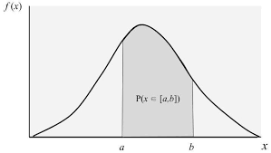
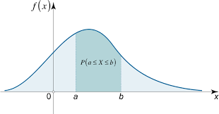
The uniform pdf is trivially a valid pdf because it is nonnegative and its integral is simply the length of the the interval on which it is nonzero, $b-a$, divided by the length. For simplicity consider the case where $a=0$ and $b=1$ so that $b-a=1$. In this case the probability of any interval
within $[0,1)$ is simply the length of the interval. The mean is easily found to be
$$
m=\int_{0}^{1} r d r=\left.\frac{r^{2}}{2}\right|{0} ^{1}=\frac{1}{2}, $$ the second moment is $$ m=\int{0}^{1} r^{2} d r=\left.\frac{r^{3}}{3}\right|{0} ^{1}=\frac{1}{3} $$ and the variance is $$ \sigma^{2}=\frac{1}{3}-\left(\frac{1}{2}\right)^{2}=\frac{1}{12} . $$ The validation of the pdf and the mean, second moment, and variance of the exponential pdf can be found from integral tables or by the integral analog to the corresponding computations for the geometric pmf, as described in appendix B. In particular, it follows from (B.9) that $$ \int{0}^{\infty} \lambda e^{-\lambda r} d r=1
$$
from (B.10) that
$$
m=\int_{0}^{\infty} r \lambda e^{-\lambda r} d r=\frac{1}{\lambda}
$$
and
$$
m^{(2)}=\int_{0}^{50} r^{2} \lambda e^{-\lambda r} d r=\frac{2}{\lambda^{2}}
$$
and hence from (2.65)
$$
\sigma^{2}=\frac{2}{\lambda^{2}}-\frac{1}{\lambda^{2}}=\frac{1}{\lambda^{2}} .
$$
The moments can also be found by integration by parts.
The Laplacian pdf is simply a mixture of an exponential pdf and its reverse, so its properties follow from those of an exponential pdf. The details are left as an exercise.
The Gaussian pdf example is more involved. In appendix B, it is shown (in the development leading up to (B.15) that
$$
\int_{-\infty}^{\infty} \frac{1}{\sqrt{2 \sigma^{2}}} e^{-\frac{(x-m)^{2}}{2 \sigma^{2}}} d x=1 .
$$
It is reasonably easy to find the mean by inspection. The function $g(x)=$ $(x-m) e^{-\frac{(x-m)^{2}}{2 \sigma^{2}}}$ is an odd function, i.e., it has the form $g(-x)=-g(x)$, and hence its integral is 0 if the integral exists at all.
统计代写|随机信号处理作业代写Statistical Signal Processing代考|Mass Functions as Densities
As in systems theory, discrete problems can be considered as continuous problems with the aid of the Dirac delta or unit impulse $\delta(t)$, a generalized function or singularity function (also, unfortunately, called a distribution) with the property that for any smooth function ${g(r) ; r \in \Re}$ and any $a \in \mathbb{R}$
$$
\int g(r) \delta(r-a) d r=g(a)
$$
Given a pmf $p$ defined on a subset of the real line $\Omega \subset \Re$, we can define a pdf $f$ by
$$
f(r)=\sum p(\omega) \delta(r-\omega)
$$
Thie ie indeed a pdf einee
$$
\begin{aligned}
\int f(r) d r &=\int\left(\sum p(\omega) \delta(r-\omega)\right) d r \
&=\sum p(\omega) \int \delta(r-\omega) d r \
&=\sum p(\omega)=1 .
\end{aligned}
$$
In a similar fashion, probabilies are computed as
$$
\begin{aligned}
\int 1_{F}(r) f(r) d r &=\int 1_{F}(r)\left(\sum p(\omega) \delta(r-\omega)\right) d r \
&=\sum p(\omega) \int 1_{F}(r) \delta(r-\omega) d r \
&=\sum p(\omega) 1_{F}(\omega)=P(F) .
\end{aligned}
$$
Given that discrete probability can be handled using the tools of continuous probability in this fashion, it is natural to inquire why not use pdf’s in both the discrete and continuous case. The main reason is simplicity, pmf’s and sums are usually simpler to handle and evaluate than pdf’s and integrals. Questions of existence and limits rarely arise, and the notation is simpler. In addition, the use of Dirac deltas assumes the theory of generalized functions in order to treat integrals involving Dirac deltas as if they were ordinary integrals, so additional mathematical machinery is required. As a result, this approach is rarely used in genuinely discrete problems. On the other hand, if one is dealing with a hybrid problem that has both discrete and continuous components, then this approach may make sense because it allows the use of a single probability function, a pdf, throughout.
统计代写|随机信号处理作业代写Statistical Signal Processing代考|Multidimensional pdf ’s
By considering multidimensional integrals we can also extend the construction of probabilities by integrals to finite-dimensional product spaces, e.g., bok $^{k}$.
Given the measurable space $\left(\Re^{k}, \mathcal{B}(\Re)^{k}\right)$, say we have a real-valued function $f$ on $R^{k}$ with the properties that
$$
\begin{gathered}
f(\mathbf{x}) \geq 0 ; \text { all } \mathbf{x}=\left(x_{0}, x_{1}, \ldots, x_{k-1}\right) \in x^{k} \
\int_{\mathfrak{R k}^{k}} f(\mathbf{x}) d \mathbf{x}=1
\end{gathered}
$$
Then define a set function $P$ by
$$
P(F)-\int_{F} f(\mathbf{x}) d \mathbf{x}, \text { all } F \in \mathcal{B}(\mathfrak{R})^{k},
$$
where the vector integral is shorthand for the $k$ – dimensional integral, that is,
$$
P(F)=\int_{\left(x_{0}, x_{1}, \ldots, x_{k-1}\right) \in F} f\left(x_{0}, x_{1}, \ldots, x_{k-1}\right) d x_{0} d x_{1} \ldots d x_{k-1}
$$

信号处理代写
统计代写|随机信号处理作业代写Statistical Signal Processing代考|Computational Examples
本节没有离散概率的对应部分详细,因为通常工程师更熟悉常用积分而不是常用和。我们将讨论限制在一些观察和多维概率计算的示例上。
统一的 pdf 是平凡有效的 pdf,因为它是非负的,并且它的积分只是它非零的区间的长度,b−一种,除以长度。为简单起见,考虑以下情况一种=0和b=1以便b−一种=1. 在这种情况下,任何区间的概率
之内[0,1)只是间隔的长度。很容易发现平均值是
米=∫01rdr=r22|01=12,第二个时刻是米=∫01r2dr=r33|01=13方差是σ2=13−(12)2=112.pdf 的验证以及指数 pdf 的均值、二阶矩和方差可以从积分表中找到,或者通过与几何 pmf 的相应计算类似的积分来找到,如附录 B 中所述。特别是,它来自(B.9) 那∫0∞λ和−λrdr=1
从(B.10)那
米=∫0∞rλ和−λrdr=1λ
和
米(2)=∫050r2λ和−λrdr=2λ2
因此从 (2.65)
σ2=2λ2−1λ2=1λ2.
也可以通过按部分积分找到矩。
拉普拉斯 pdf 只是指数 pdf 及其反转的混合,因此它的属性遵循指数 pdf 的属性。细节留作练习。
高斯 pdf 示例涉及更多。在附录 B 中,显示(在 (B.15) 之前的开发中)
∫−∞∞12σ2和−(X−米)22σ2dX=1.
通过检查很容易找到平均值。功能G(X)= (X−米)和−(X−米)22σ2是一个奇函数,即它的形式为G(−X)=−G(X),因此如果积分存在,则其积分为 0。
统计代写|随机信号处理作业代写Statistical Signal Processing代考|Mass Functions as Densities
与系统理论一样,离散问题可以在狄拉克三角洲或单位脉冲的帮助下被视为连续问题d(吨),一个广义函数或奇异函数(不幸的是,也称为分布),其属性对于任何平滑函数G(r);r∈ℜ和任何一种∈R
∫G(r)d(r−一种)dr=G(一种)
给定一个 pmfp在实线的子集上定义Ω⊂ℜ,我们可以定义一个pdfF经过
F(r)=∑p(ω)d(r−ω)
Thie ie 确实是一个 pdf einee
∫F(r)dr=∫(∑p(ω)d(r−ω))dr =∑p(ω)∫d(r−ω)dr =∑p(ω)=1.
以类似的方式,概率计算为
∫1F(r)F(r)dr=∫1F(r)(∑p(ω)d(r−ω))dr =∑p(ω)∫1F(r)d(r−ω)dr =∑p(ω)1F(ω)=磷(F).
鉴于可以以这种方式使用连续概率工具处理离散概率,很自然地询问为什么不在离散和连续情况下使用 pdf。主要原因是简单,pmf 和 sum 通常比 pdf 和积分更容易处理和评估。存在和限制的问题很少出现,符号更简单。此外,狄拉克三角洲的使用假设了广义函数理论,以便将涉及狄拉克三角洲的积分视为普通积分,因此需要额外的数学机制。因此,这种方法很少用于真正离散的问题。另一方面,如果要处理具有离散和连续分量的混合问题,
统计代写|随机信号处理作业代写Statistical Signal Processing代考|Multidimensional pdf ’s
通过考虑多维积分,我们还可以将积分的概率构造扩展到有限维乘积空间,例如 bokķ.
给定可测量的空间(ℜķ,乙(ℜ)ķ),假设我们有一个实值函数F在Rķ具有以下属性
F(X)≥0; 全部 X=(X0,X1,…,Xķ−1)∈Xķ ∫RķķF(X)dX=1
然后定义一个集合函数磷经过
磷(F)−∫FF(X)dX, 全部 F∈乙(R)ķ,
其中向量积分是ķ– 维积分,即,
磷(F)=∫(X0,X1,…,Xķ−1)∈FF(X0,X1,…,Xķ−1)dX0dX1…dXķ−1

统计代写请认准statistics-lab™. statistics-lab™为您的留学生涯保驾护航。
金融工程代写
金融工程是使用数学技术来解决金融问题。金融工程使用计算机科学、统计学、经济学和应用数学领域的工具和知识来解决当前的金融问题,以及设计新的和创新的金融产品。
非参数统计代写
非参数统计指的是一种统计方法,其中不假设数据来自于由少数参数决定的规定模型;这种模型的例子包括正态分布模型和线性回归模型。
广义线性模型代考
广义线性模型(GLM)归属统计学领域,是一种应用灵活的线性回归模型。该模型允许因变量的偏差分布有除了正态分布之外的其它分布。
术语 广义线性模型(GLM)通常是指给定连续和/或分类预测因素的连续响应变量的常规线性回归模型。它包括多元线性回归,以及方差分析和方差分析(仅含固定效应)。
有限元方法代写
有限元方法(FEM)是一种流行的方法,用于数值解决工程和数学建模中出现的微分方程。典型的问题领域包括结构分析、传热、流体流动、质量运输和电磁势等传统领域。
有限元是一种通用的数值方法,用于解决两个或三个空间变量的偏微分方程(即一些边界值问题)。为了解决一个问题,有限元将一个大系统细分为更小、更简单的部分,称为有限元。这是通过在空间维度上的特定空间离散化来实现的,它是通过构建对象的网格来实现的:用于求解的数值域,它有有限数量的点。边界值问题的有限元方法表述最终导致一个代数方程组。该方法在域上对未知函数进行逼近。[1] 然后将模拟这些有限元的简单方程组合成一个更大的方程系统,以模拟整个问题。然后,有限元通过变化微积分使相关的误差函数最小化来逼近一个解决方案。
tatistics-lab作为专业的留学生服务机构,多年来已为美国、英国、加拿大、澳洲等留学热门地的学生提供专业的学术服务,包括但不限于Essay代写,Assignment代写,Dissertation代写,Report代写,小组作业代写,Proposal代写,Paper代写,Presentation代写,计算机作业代写,论文修改和润色,网课代做,exam代考等等。写作范围涵盖高中,本科,研究生等海外留学全阶段,辐射金融,经济学,会计学,审计学,管理学等全球99%专业科目。写作团队既有专业英语母语作者,也有海外名校硕博留学生,每位写作老师都拥有过硬的语言能力,专业的学科背景和学术写作经验。我们承诺100%原创,100%专业,100%准时,100%满意。
随机分析代写
随机微积分是数学的一个分支,对随机过程进行操作。它允许为随机过程的积分定义一个关于随机过程的一致的积分理论。这个领域是由日本数学家伊藤清在第二次世界大战期间创建并开始的。
时间序列分析代写
随机过程,是依赖于参数的一组随机变量的全体,参数通常是时间。 随机变量是随机现象的数量表现,其时间序列是一组按照时间发生先后顺序进行排列的数据点序列。通常一组时间序列的时间间隔为一恒定值(如1秒,5分钟,12小时,7天,1年),因此时间序列可以作为离散时间数据进行分析处理。研究时间序列数据的意义在于现实中,往往需要研究某个事物其随时间发展变化的规律。这就需要通过研究该事物过去发展的历史记录,以得到其自身发展的规律。
回归分析代写
多元回归分析渐进(Multiple Regression Analysis Asymptotics)属于计量经济学领域,主要是一种数学上的统计分析方法,可以分析复杂情况下各影响因素的数学关系,在自然科学、社会和经济学等多个领域内应用广泛。
MATLAB代写
MATLAB 是一种用于技术计算的高性能语言。它将计算、可视化和编程集成在一个易于使用的环境中,其中问题和解决方案以熟悉的数学符号表示。典型用途包括:数学和计算算法开发建模、仿真和原型制作数据分析、探索和可视化科学和工程图形应用程序开发,包括图形用户界面构建MATLAB 是一个交互式系统,其基本数据元素是一个不需要维度的数组。这使您可以解决许多技术计算问题,尤其是那些具有矩阵和向量公式的问题,而只需用 C 或 Fortran 等标量非交互式语言编写程序所需的时间的一小部分。MATLAB 名称代表矩阵实验室。MATLAB 最初的编写目的是提供对由 LINPACK 和 EISPACK 项目开发的矩阵软件的轻松访问,这两个项目共同代表了矩阵计算软件的最新技术。MATLAB 经过多年的发展,得到了许多用户的投入。在大学环境中,它是数学、工程和科学入门和高级课程的标准教学工具。在工业领域,MATLAB 是高效研究、开发和分析的首选工具。MATLAB 具有一系列称为工具箱的特定于应用程序的解决方案。对于大多数 MATLAB 用户来说非常重要,工具箱允许您学习和应用专业技术。工具箱是 MATLAB 函数(M 文件)的综合集合,可扩展 MATLAB 环境以解决特定类别的问题。可用工具箱的领域包括信号处理、控制系统、神经网络、模糊逻辑、小波、仿真等。