ELEC 531 - 统计代写答疑辅导

标签： ELEC 531

统计代写|随机信号处理作业代写Statistical Signal Processing代考|Random Processes

Posted on 2022年5月3日2022年5月3日 by statistics-lab

如果你也在怎样代写随机信号处理Statistical Signal Processing这个学科遇到相关的难题，请随时右上角联系我们的24/7代写客服。

随机信号处理是一种将信号视为随机过程的方法，利用其统计特性来执行信号处理任务。

statistics-lab™ 为您的留学生涯保驾护航在代写随机信号处理Statistical Signal Processing方面已经树立了自己的口碑, 保证靠谱, 高质且原创的统计Statistics代写服务。我们的专家在代写随机信号处理Statistical Signal Processing代写方面经验极为丰富，各种代写随机信号处理Statistical Signal Processing相关的作业也就用不着说。

我们提供的随机信号处理Statistical Signal Processingl及其相关学科的代写，服务范围广, 其中包括但不限于:

Statistical Inference 统计推断
Statistical Computing 统计计算
Advanced Probability Theory 高等概率论
Advanced Mathematical Statistics 高等数理统计学
(Generalized) Linear Models 广义线性模型
Statistical Machine Learning 统计机器学习
Longitudinal Data Analysis 纵向数据分析
Foundations of Data Science 数据科学基础

统计代写|随机信号处理作业代写Statistical Signal Processing代考|Random Processes

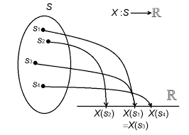
It is straightforward conceptually to go from one random variable to $k$ random variables constituting a $k$-dimensional random vector. It is perhaps a greater leap to extend the idea to a random process. The idea is at least easy to state, but it will take more work to provide examples and the mathematical details will prove more complicated. A random process is a sequence of random variables $\left{X_{n} ; n=0,1, \ldots\right}$ defined on a common experiment. It can be thought of as an infinite dimensional random vector. To be more accurate, this is an example of a discrete-time, one-sided random process. It is called “discrete-time” because the index $n$ which corresponds to time takes on discrete values (here the nonnegative integers) and it is called “one-sided” because only nonnegative times are allowed. A discrete-time random process is also called a time series in the statistics literature and it is often denoted as ${X(n) n=0,1, \ldots}$ and is sometimes denoted by ${X[n]}$ in the digital signal processing literature. Two questions might oocur to the reader: how does one construct an infinite family of random variables on a single experiment? How can one provide a direct development of a random process as accomplished for random variables and vectors? The direct development might appear hopeless since infinite dimensional vectors are involved.

The first problem is reasonably easy to handle by example. Consider the usual uniform pdf experiment. Rename the random variables $Y$ and $W$ as $X_{0}$ and $X_{1}$, respectively. Consider the following definition of an infinite family of random variables $X_{n}:[0,1) \rightarrow{0,1}$ for $n=0,1, \ldots$. Every $r \in[0,1)$ can be expanded as a binary expansion of the form
$$
r=\sum_{n=0}^{\infty} b_{n}(r) 2^{-n-1}
$$
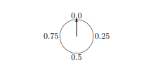
This simply replaces the usual decimal representation by a binary representation. For example, $1 / 4$ is $.25$ in decimal and .01 or .010000… in binary. $1 / 2$ is .5 in decimal and yields the binary sequence .1000…, $1 / 4$ is $.25$ in decimal and yields the binary sequence .0100…, $3 / 4$ is .75 in decimal and $.11000 \ldots .$ and $1 / 3$ is $.3333 . . .$ in decimal and $.010101 \ldots$ in binary.

Define the random process by $X_{n}(r)=b_{n}(r)$, that is, the $n$th term in the binary expansion of $r$. When $n=0,1$ this reduces to the specific $X_{0}$ and $X_{1}$ already considered.

统计代写|随机信号处理作业代写Statistical Signal Processing代考|Random Variables

We now develop the promised precise definition of a random variable. As you might guess, a technical condition for random variables is required because of certain subtle pathological problems that have to do with the ability to determine probabilities for the random variable. To arrive at the precise definition, we start with the informal definition of a random variable that we have already given and then show the inevitable difficulty that results without the technical condition. We have informally defined a

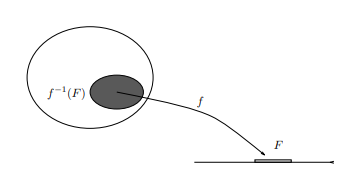
random variable as being a function on a sample space. Suppose we have a probability space $(\Omega, \mathcal{F}, P)$. Let $f: \Omega \rightarrow \Re$ be a function mapping the same space into the real line so that $f$ is a candidate for a random variable. Since the selection of the original sample point $\omega$ is random, that is, governed by a probability measure, so should be the output of our measurement of random variable $f(\omega)$. That is, we should be able to find the probability of an “output event” such as the event “the outcome of the random variable $f$ was between $a$ and $b, “$ that is, the event $F \subset \Re$ given by $F=(a, b)$. Observe that there are two different kinds of events being considered here:

output events or members of the event space of the range or range space of the random variable, that is, events consisting of subsets of possible output values of the random variable; and
input events or $\Omega$ events, events in the original sample space of the original probability space.

Can we find the probability of this output event? That is, can we make mathematieal senee out of the quantity “the probability that $f$ areumee a value in an event $F \subset \Re$ ?? On reflection it seems clear that we can. The probability that $f$ assumes a value in some set of values must be the probability of all values in the original sample space that result in a value of $f$ in the given set. We will make this concept more precise shortly. To save writing we will abbreviate such English statements to the form $\operatorname{Pr}(f \in F)$, or $\operatorname{Pr}(F)$, that is, when the notation $\operatorname{Pr}(F)$ is encountered it should be interpreted as shorthand for the English statement for “the probability of an event $F^{” \prime}$ or “the probability that the event $F$ will occur” and not as a precise mathematical quantity.

统计代写|随机信号处理作业代写Statistical Signal Processing代考|Distributions of Random Variables

Suppose we have a probability space $(\Omega, \mathcal{F}, P)$ with a random variable, $X$, defined on the space. The random variable $X$ takes values on its range space which is some subset $A$ of $\Re$ (possibly $A=\Re$ ). The range space $A$ of a random variable is often called the alphabet of the random variable. As we have seen, since $X$ is a random variable, we know that all subsets of $\Omega$ of the form $X^{-1}(F)={\omega: X(\omega) \in F}$, with $F \in B(A)$, must be members of $\mathcal{F}$ by definition. Thus the set function $P_{X}$ defined by
$$
P_{X}(F)=P\left(X^{-1}(F)\right)=P({\omega: X(\omega) \in F}) ; F \in \mathcal{B}(A)
$$
is well defined and assigns probabilities to output events involving the random variable in terms of the original probability of input events in the orig-

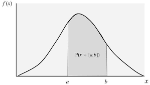
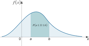
inal experiment. The three written forms in equation (3.22) are all read as $\operatorname{Pr}(X \in F)$ or “the probability that the random variable $X$ takes on a value in $F .$ Furthermore, since inverse images preserve all set-theoretic operations (see problem A.12), $P_{X}$ satisfies the axioms of probability as a probability measure on $(A, \mathcal{B}(A))-$ it is nonnegative, $P_{X}(A)=1$, and it is countably additive. Thus $P_{X}$ is a probability measure on the measurable space $(A, \mathcal{B}(A))$. Therefore, given a probability space and a random variable $X$, we have constructed a new probability space $\left(A, \mathcal{B}(A), P_{X}\right)$ where the events describe outcomes of the random variable. The probability measure $P_{X}$ is called the distribution of $X$ (as opposed to a “cumulative distribution function” of $X$ to be introduced later).

If two random variables have the same distribution, then they are said to be equivalent since they have the same probabilistic description, whether or not they are defined on the same underlying space or have the same functional form (see problem 3.22).

A substantial part of the application of probability theory to practical probblems is devoted to determining the distributions of random variables, perfurmaing the “ealeulus of prubabsility.” Ons bugina with a probubility space. A random variable is defined on that space. The distribution of the random variable is then derived, and this results in a new probability space. This topic is called variously “derived distributions” or “transformations of random variables” and is often developed in the literature as a sequence of apparently unrelated subjects. When the points in the original sample space can be interpreted as “signals,” then such problems can be viewed as “signal processing” and derived distribution problems are fundamental to the analysis of statistical signal processing systems. We shall emphasize that all such examples are just applications of the basic inverse image formula (3.22) and form a unified whole. In fact, this formula, with its vector analog, is one of the most important in applications of probability theory. Its specialization to discrete input spaces using sums and to continuous input spaces using integrals will be seen and used often throughout this book.

信号处理代写

统计代写|随机信号处理作业代写Statistical Signal Processing代考|Random Processes

从一个随机变量到ķ随机变量构成ķ维随机向量。将这个想法扩展到随机过程可能是一个更大的飞跃。这个想法至少很容易陈述，但提供示例需要更多的工作，并且数学细节将被证明更加复杂。随机过程是一系列随机变量\左{X_{n} ; n=0,1, \ldots\right}\左{X_{n} ; n=0,1, \ldots\right}定义在一个共同的实验上。它可以被认为是一个无限维的随机向量。更准确地说，这是离散时间、单边随机过程的一个示例。它被称为“离散时间”，因为索引n它对应于时间的离散值（这里是非负整数），它被称为“单面”，因为只允许非负时间。离散时间随机过程在统计学文献中也称为时间序列，通常表示为X(n)n=0,1,…有时表示为X[n]在数字信号处理文献中。读者可能会想到两个问题：如何在一次实验中构建无限的随机变量族？如何提供对随机变量和向量完成的随机过程的直接开发？由于涉及无限维向量，直接发展可能看起来没有希望。

第一个问题很容易通过示例来处理。考虑通常的统一 pdf 实验。重命名随机变量是和在作为X0和X1，分别。考虑以下无限随机变量族的定义Xn:[0,1)→0,1为了n=0,1,…. 每一个r∈[0,1)可以展开为形式的二进制展开
r=∑n=0∞bn(r)2−n−1
这只是用二进制表示代替了通常的十进制表示。例如，1/4是.25十进制和 .01 或 .010000… 二进制。1/2是十进制的 0.5 并产生二进制序列 .1000…，1/4是.25十进制并产生二进制序列 .0100…,3/4十进制为 0.75 和.11000….和1/3是.3333…十进制和.010101…在二进制。

定义随机过程Xn(r)=bn(r)，那就是n的二进制展开中的第项r. 什么时候n=0,1这减少到具体X0和X1已经考虑过了。

统计代写|随机信号处理作业代写Statistical Signal Processing代考|Random Variables

我们现在开发了随机变量的承诺精确定义。正如您可能猜到的那样，由于某些微妙的病理问题与确定随机变量概率的能力有关，因此需要随机变量的技术条件。为了得到精确的定义，我们从已经给出的随机变量的非正式定义开始，然后展示在没有技术条件的情况下产生的不可避免的困难。我们非正式地定义了一个

随机变量作为样本空间上的函数。假设我们有一个概率空间(Ω,F,磷). 让F:Ω→ℜ是一个将相同空间映射到实线的函数，使得F是随机变量的候选者。由于原始样本点的选择ω是随机的，即由概率测度控制，因此我们对随机变量的测度的输出也应该是F(ω). 也就是说，我们应该能够找到“输出事件”的概率，例如事件“随机变量的结果”F介于一种和b,“也就是事件F⊂ℜ由F=(一种,b). 请注意，这里考虑了两种不同类型的事件：

输出事件或随机变量的范围或范围空间的事件空间的成员，即由随机变量的可能输出值的子集组成的事件；和
输入事件或Ω事件，原始概率空间的原始样本空间中的事件。

我们能找到这个输出事件的概率吗？也就是说，我们能否从数量“概率Fareumee 事件中的值F⊂ℜ?? 经过反思，我们似乎很清楚我们可以。的概率F假设一组值中的一个值必须是原始样本空间中所有值的概率F在给定的集合中。我们将很快使这个概念更加精确。为了节省书写，我们会将此类英文陈述缩写为表格公关⁡(F∈F)，或者公关⁡(F)，也就是说，当符号公关⁡(F)遇到它应该被解释为英语语句“事件的概率”的简写F”′或“事件发生的概率F会发生”，而不是作为一个精确的数学量。

统计代写|随机信号处理作业代写Statistical Signal Processing代考|Distributions of Random Variables

假设我们有一个概率空间(Ω,F,磷)带有随机变量，X，在空间上定义。随机变量X在其范围空间上取值，该范围空间是某个子集一种的ℜ（可能一种=ℜ）。范围空间一种随机变量的字母表通常称为随机变量的字母表。正如我们所见，自从X是一个随机变量，我们知道所有的子集Ω形式的X−1(F)=ω:X(ω)∈F，和F∈乙(一种), 必须是F根据定义。因此设置函数磷X被定义为
磷X(F)=磷(X−1(F))=磷(ω:X(ω)∈F);F∈乙(一种)
定义良好，并根据原始输入事件的原始概率为涉及随机变量的输出事件分配概率

最终实验。等式（3.22）中的三个书面形式都读作公关⁡(X∈F)或“随机变量的概率X取值F.此外，由于逆图像保留了所有集合论操作（见问题 A.12），磷X满足概率公理作为概率度量(一种,乙(一种))−它是非负的，磷X(一种)=1, 并且是可数相加的。因此磷X是可测空间上的概率测度(一种,乙(一种)). 因此，给定一个概率空间和一个随机变量X，我们构造了一个新的概率空间(一种,乙(一种),磷X)其中事件描述随机变量的结果。概率测度磷X称为分布X（相对于“累积分布函数”X稍后介绍）。

如果两个随机变量具有相同的分布，则称它们是等价的，因为它们具有相同的概率描述，无论它们是否定义在相同的基础空间或具有相同的函数形式（参见问题 3.22）。

将概率论应用于实际问题的很大一部分致力于确定随机变量的分布，从而实现“概率论”。带有概率空间的 Ons bugina。在该空间上定义了一个随机变量。然后导出随机变量的分布，这会产生一个新的概率空间。这个主题被称为不同的“派生分布”或“随机变量的变换”，并且通常在文献中被发展为一系列明显不相关的主题。当原始样本空间中的点可以解释为“信号”时，则可以将此类问题视为“信号处理”，而派生的分布问题是统计信号处理系统分析的基础。我们要强调的是，所有这些例子都只是基本逆像公式（3.22）的应用，形成了一个统一的整体。事实上，这个公式及其矢量类比是概率论应用中最重要的公式之一。它专门针对使用求和的离散输入空间和使用积分的连续输入空间将在本书中经常看到和使用。

统计代写|随机信号处理作业代写Statistical Signal Processing代考请认准statistics-lab™

统计代写请认准statistics-lab™. statistics-lab™为您的留学生涯保驾护航。

金融工程代写

金融工程是使用数学技术来解决金融问题。金融工程使用计算机科学、统计学、经济学和应用数学领域的工具和知识来解决当前的金融问题，以及设计新的和创新的金融产品。

非参数统计代写

非参数统计指的是一种统计方法，其中不假设数据来自于由少数参数决定的规定模型；这种模型的例子包括正态分布模型和线性回归模型。

广义线性模型代考

广义线性模型（GLM）归属统计学领域，是一种应用灵活的线性回归模型。该模型允许因变量的偏差分布有除了正态分布之外的其它分布。

术语广义线性模型（GLM）通常是指给定连续和/或分类预测因素的连续响应变量的常规线性回归模型。它包括多元线性回归，以及方差分析和方差分析（仅含固定效应）。

有限元方法代写

有限元方法（FEM）是一种流行的方法，用于数值解决工程和数学建模中出现的微分方程。典型的问题领域包括结构分析、传热、流体流动、质量运输和电磁势等传统领域。

有限元是一种通用的数值方法，用于解决两个或三个空间变量的偏微分方程（即一些边界值问题）。为了解决一个问题，有限元将一个大系统细分为更小、更简单的部分，称为有限元。这是通过在空间维度上的特定空间离散化来实现的，它是通过构建对象的网格来实现的：用于求解的数值域，它有有限数量的点。边界值问题的有限元方法表述最终导致一个代数方程组。该方法在域上对未知函数进行逼近。[1] 然后将模拟这些有限元的简单方程组合成一个更大的方程系统，以模拟整个问题。然后，有限元通过变化微积分使相关的误差函数最小化来逼近一个解决方案。

tatistics-lab作为专业的留学生服务机构，多年来已为美国、英国、加拿大、澳洲等留学热门地的学生提供专业的学术服务，包括但不限于Essay代写，Assignment代写，Dissertation代写，Report代写，小组作业代写，Proposal代写，Paper代写，Presentation代写，计算机作业代写，论文修改和润色，网课代做，exam代考等等。写作范围涵盖高中，本科，研究生等海外留学全阶段，辐射金融，经济学，会计学，审计学，管理学等全球99%专业科目。写作团队既有专业英语母语作者，也有海外名校硕博留学生，每位写作老师都拥有过硬的语言能力，专业的学科背景和学术写作经验。我们承诺100%原创，100%专业，100%准时，100%满意。

随机分析代写

随机微积分是数学的一个分支，对随机过程进行操作。它允许为随机过程的积分定义一个关于随机过程的一致的积分理论。这个领域是由日本数学家伊藤清在第二次世界大战期间创建并开始的。

时间序列分析代写

随机过程，是依赖于参数的一组随机变量的全体，参数通常是时间。随机变量是随机现象的数量表现，其时间序列是一组按照时间发生先后顺序进行排列的数据点序列。通常一组时间序列的时间间隔为一恒定值（如1秒，5分钟，12小时，7天，1年），因此时间序列可以作为离散时间数据进行分析处理。研究时间序列数据的意义在于现实中，往往需要研究某个事物其随时间发展变化的规律。这就需要通过研究该事物过去发展的历史记录，以得到其自身发展的规律。

回归分析代写

多元回归分析渐进（Multiple Regression Analysis Asymptotics）属于计量经济学领域，主要是一种数学上的统计分析方法，可以分析复杂情况下各影响因素的数学关系，在自然科学、社会和经济学等多个领域内应用广泛。

MATLAB代写

MATLAB 是一种用于技术计算的高性能语言。它将计算、可视化和编程集成在一个易于使用的环境中，其中问题和解决方案以熟悉的数学符号表示。典型用途包括：数学和计算算法开发建模、仿真和原型制作数据分析、探索和可视化科学和工程图形应用程序开发，包括图形用户界面构建MATLAB 是一个交互式系统，其基本数据元素是一个不需要维度的数组。这使您可以解决许多技术计算问题，尤其是那些具有矩阵和向量公式的问题，而只需用 C 或 Fortran 等标量非交互式语言编写程序所需的时间的一小部分。MATLAB 名称代表矩阵实验室。MATLAB 最初的编写目的是提供对由 LINPACK 和 EISPACK 项目开发的矩阵软件的轻松访问，这两个项目共同代表了矩阵计算软件的最新技术。MATLAB 经过多年的发展，得到了许多用户的投入。在大学环境中，它是数学、工程和科学入门和高级课程的标准教学工具。在工业领域，MATLAB 是高效研究、开发和分析的首选工具。MATLAB 具有一系列称为工具箱的特定于应用程序的解决方案。对于大多数 MATLAB 用户来说非常重要，工具箱允许您学习和应用专业技术。工具箱是 MATLAB 函数（M 文件）的综合集合，可扩展 MATLAB 环境以解决特定类别的问题。可用工具箱的领域包括信号处理、控制系统、神经网络、模糊逻辑、小波、仿真等。

R语言代写	问卷设计与分析代写
PYTHON代写	回归分析与线性模型代写
MATLAB代写	方差分析与试验设计代写
STATA代写	机器学习/统计学习代写
SPSS代写	计量经济学代写
EVIEWS代写	时间序列分析代写
EXCEL代写	深度学习代写
SQL代写	各种数据建模与可视化代写

统计代写|随机信号处理作业代写Statistical Signal Processing代考|Random Variables, Vectors, and Processes

Posted on 2022年5月3日2022年5月3日 by statistics-lab

如果你也在怎样代写随机信号处理Statistical Signal Processing这个学科遇到相关的难题，请随时右上角联系我们的24/7代写客服。

随机信号处理是一种将信号视为随机过程的方法，利用其统计特性来执行信号处理任务。

我们提供的随机信号处理Statistical Signal Processingl及其相关学科的代写，服务范围广, 其中包括但不限于:

Statistical Inference 统计推断
Statistical Computing 统计计算
Advanced Probability Theory 高等概率论
Advanced Mathematical Statistics 高等数理统计学
(Generalized) Linear Models 广义线性模型
Statistical Machine Learning 统计机器学习
Longitudinal Data Analysis 纵向数据分析
Foundations of Data Science 数据科学基础

5.1 Random variable and probability distribution - definitions | STAT 101 IPS (WSMiP UŁ) — 统计代写|随机信号处理作业代写Statistical Signal Processing代考|Random Variables, Vectors, and Processes

统计代写|随机信号处理作业代写Statistical Signal Processing代考|Random Variables

The name random variable suggests a variable that takes on values randomly. In a loose, intuitive way this is the right interpretation – e.g., an observer who is measuring the amount of noise on a communication link sees a random variable in this sense. We require, however, a more precise mathematical definition for analytical purposes. Mathematically a random variable is neither random nor a variable – it is just a function mapping one sample space into another space. The first space is the sample space portion of a probability space, and the second space is a subset of the real line (some authors wotld call this a “real-valued” random variable). The careful mathematical definition will place a constraint on the function to ensure that the theory makes sense, but for the moment we will adopt the informal definition that a random variable is just a function.

A random variable is perhaps best thought of as a measurement on a

probability space; that is, for each sample point $\omega$ the random variable produces some value, denoted functionally as $f(\omega)$. One can view $\omega$ as the result of some experiment and $f(\omega)$ as the restalt of a measurement made on the experiment, as in the example of the simple binary quantizer introduced in the introduction to chapter 2 . The experiment outcome $\omega$ is from an abstract space, e.g., real numbers, integers, ASCII characters, waveforms, sequences, Chinese characters, etc. The resulting value of the measurement or random variable $f(\omega)$, however, must be “concrete” in the sense of being a real number, e.g., a meter reading. The randomness is all in the original probability space and not in the random variable; that is, once the $\omega$ is selected in a “random” way, the output value of sample value of the random variable is determined.

Alternatively, the original point $\omega$ can be viewed as an “input signal” and the random variable $f$ can be viewed as “signal processing,” i.e., the input signal $\omega$ is converted into an “output signal” $f(\omega)$ by the random variable. This viewpoint becomes both precise and relevant when we indeed choose our original sample space to be a signal space and we generalize random variables by random vectors and processes.

Before proceeding to the formal definition of random variables, vectors, and processes, we motivate several of the basic ideas by simple examples, beginning with random variables constructed on the fair wheel experiment of the introduction to chapter 2 .

统计代写|随机信号处理作业代写Statistical Signal Processing代考|A Coin Flip

We have already encountered an example of a random variable in the introduction to chapter 2 , where we defined a random variable $q$ on the spinning wheel experiment which produced an output with the same pmf as a uniform coin flip. We begin by summarizing the idea with some slight notational changes and then consider the implications in additional detail.
Begin with a probability space $(\Omega, \mathcal{F}, P)$ where $\Omega=\Re$ and the probability $P$ is defined by (2.2) using the uniform pdf on $[0,1)$ of (2.4) Define the function $Y: \Re \rightarrow{0,1}$ by
$$
Y(r)= \begin{cases}0 & \text { if } r \leq 0.5 \ 1 & \text { otherwise }\end{cases}
$$
When Tyche performs the experiment of spinning the pointer, we do not actually observe the pointer, but only the resulting binary value of $Y$. $Y$ can be thought of as signal processing or as a measurement on the original experiment. Subject to a technical constraint to be introduced later, any function defined on the sample space of an experiment is called a random

variable. The “randomness” of a random variable is “inherited” from the underlying experiment and in theory the probability measure describing its outputs should be derivable from the initial probability space and the structure of the function. To avoid confusion with the probability measure $P$ of the original experiment, refer to the probability measure associated with outcomes of $Y$ as $P_{Y} . P_{Y}$ is called the distribution of the random variable $Y$. The probability $P_{Y}(F)$ can be defined in a natural way as the probability computed using $P$ of all the original samples that are mapped by $Y$ into the subset $F$ :
$$
P_{Y}(F)=P({r: Y(r) \in F})
$$

统计代写|随机信号处理作业代写Statistical Signal Processing代考|Random Vectors

The issue of the possible equality of two random variables raises an interesting point. If you are told that $Y$ and $V$ are two separate random variables with pm’t’s $p_{Y}$ and $p_{V}$, then the quegtion of whether or not they are equivalent can be answered from these pmf’s alone. If you wish to determine whether or not the two random variables are in fact equal, however, then they must be considered together or jointly. In the case where we have a random variable $Y$ with outcomes in ${0,1}$ and a random variable $V$ with outcomes in ${0,1}$, we could consider the two together as a single random vector ${Y, V}$ with outcomes in the Cartesian product space $\Omega_{Y V}={0,1}^{2} \triangleq{(0,0),(0,1),(1,0),(1,1)}$ with some pmf $p_{Y, V}$ describing the combined behavior
$$
p_{Y, V}(y, v)=\operatorname{Pr}(Y=y, V=v)
$$
so that
$$
\operatorname{Pr}((Y, V) \in F)=\sum_{y, v:(y, v) \in F} p_{Y, V}(y, v) ; F \in \mathcal{B}{Y V}, $$ where in this simple discrete problem we take the event space $\mathcal{B}{Y V}$ to be the power set of $\Omega_{Y V}$. Now the question of equality makes sense as we can evaluate the probability that the two are equal:
$$
\operatorname{Pr}(Y=V)=\sum_{y, v \in Y-v} p_{Y, V}(y, v) .
$$
If this probability is 1 , then we know that the two random variables are in fact equal with probability $1 .$

Chapter 2 Discrete random variables | Notes for Probability — 统计代写|随机信号处理作业代写Statistical Signal Processing代考|Random Variables, Vectors, and Processes

信号处理代写

统计代写|随机信号处理作业代写Statistical Signal Processing代考|Random Variables

随机变量的名称暗示了一个随机取值的变量。以一种松散、直观的方式，这是正确的解释——例如，测量通信链路上的噪声量的观察者在这个意义上看到了一个随机变量。然而，为了分析的目的，我们需要一个更精确的数学定义。从数学上讲，随机变量既不是随机变量也不是变量——它只是一个将一个样本空间映射到另一个空间的函数。第一个空间是概率空间的样本空间部分，第二个空间是实线的子集（一些作者称其为“实值”随机变量）。仔细的数学定义将对函数施加约束，以确保理论有意义，

随机变量也许最好被认为是对

概率空间；也就是说，对于每个样本点ω随机变量产生一些值，在功能上表示为F(ω). 一个可以查看ω作为一些实验的结果和F(ω)作为对实验进行测量的重新设置，如第 2 章介绍中介绍的简单二进制量化器的示例。实验结果ω来自抽象空间，例如实数、整数、ASCII字符、波形、序列、汉字等。测量或随机变量的结果值F(ω)然而，在实数的意义上，它必须是“具体的”，例如，仪表读数。随机性都在原始概率空间中，而不是在随机变量中；也就是说，一旦ω以“随机”的方式选择，确定随机变量的样本值的输出值。

或者，原点ω可以看作是“输入信号”和随机变量F可以看作是“信号处理”，即输入信号ω转换成“输出信号”F(ω)由随机变量。当我们确实选择我们的原始样本空间作为信号空间并且我们通过随机向量和过程来概括随机变量时，这个观点变得既精确又相关。

在开始正式定义随机变量、向量和过程之前，我们通过简单的例子来激发几个基本的想法，从第 2 章引言的公平轮实验中构建的随机变量开始。

统计代写|随机信号处理作业代写Statistical Signal Processing代考|A Coin Flip

我们已经在第 2 章的介绍中遇到了一个随机变量的例子，我们在其中定义了一个随机变量。q在旋转轮实验中，该实验产生的输出与均匀抛硬币具有相同的 pmf。我们首先通过一些细微的符号变化来总结这个想法，然后更详细地考虑其含义。
从概率空间开始(Ω,F,磷)在哪里Ω=ℜ和概率磷由 (2.2) 使用统一的 pdf 定义[0,1)(2.4)定义函数是:ℜ→0,1经过
是(r)={0 如果 r≤0.5 1 除此以外
当 Tyche 进行旋转指针的实验时，我们实际上并没有观察到指针，而只是观察到的二进制值是. 是可以认为是信号处理或对原始实验的测量。受限于稍后介绍的技术约束，在实验的样本空间上定义的任何函数都称为随机

多变的。随机变量的“随机性”是从基础实验“继承”的，理论上描述其输出的概率度量应该可以从初始概率空间和函数结构推导出来。避免与概率测度混淆磷原始实验的，指的是与结果相关的概率测度是作为磷是.磷是称为随机变量的分布是. 概率磷是(F)可以以自然的方式定义为使用计算的概率磷映射的所有原始样本是进入子集F :
磷是(F)=磷(r:是(r)∈F)

统计代写|随机信号处理作业代写Statistical Signal Processing代考|Random Vectors

两个随机变量可能相等的问题提出了一个有趣的观点。如果你被告知是和在是两个独立的随机变量，带有 pm’t’sp是和p在，那么它们是否等效的问题可以仅从这些 pmf 中回答。但是，如果您希望确定两个随机变量实际上是否相等，则必须将它们一起或共同考虑。在我们有一个随机变量的情况下是结果在0,1和一个随机变量在结果在0,1，我们可以将两者一起视为单个随机向量是,在在笛卡尔积空间中产生结果Ω是在=0,12≜(0,0),(0,1),(1,0),(1,1)有一些 pmfp是,在描述组合行为
p是,在(是,在)=公关⁡(是=是,在=在)
以便
公关⁡((是,在)∈F)=∑是,在:(是,在)∈Fp是,在(是,在);F∈乙是在,在这个简单的离散问题中，我们采用事件空间乙是在成为的幂集Ω是在. 现在相等的问题是有道理的，因为我们可以评估两者相等的概率：
公关⁡(是=在)=∑是,在∈是−在p是,在(是,在).
如果这个概率是 1 ，那么我们知道这两个随机变量实际上是概率相等的1.

统计代写请认准statistics-lab™. statistics-lab™为您的留学生涯保驾护航。

金融工程代写

非参数统计代写

非参数统计指的是一种统计方法，其中不假设数据来自于由少数参数决定的规定模型；这种模型的例子包括正态分布模型和线性回归模型。

广义线性模型代考

广义线性模型（GLM）归属统计学领域，是一种应用灵活的线性回归模型。该模型允许因变量的偏差分布有除了正态分布之外的其它分布。

有限元方法代写

随机分析代写

时间序列分析代写

回归分析代写

MATLAB代写

R语言代写	问卷设计与分析代写
PYTHON代写	回归分析与线性模型代写
MATLAB代写	方差分析与试验设计代写
STATA代写	机器学习/统计学习代写
SPSS代写	计量经济学代写
EVIEWS代写	时间序列分析代写
EXCEL代写	深度学习代写
SQL代写	各种数据建模与可视化代写

统计代写|随机信号处理作业代写Statistical Signal Processing代考|Independence

Posted on 2022年5月3日2022年5月3日 by statistics-lab

如果你也在怎样代写随机信号处理Statistical Signal Processing这个学科遇到相关的难题，请随时右上角联系我们的24/7代写客服。

随机信号处理是一种将信号视为随机过程的方法，利用其统计特性来执行信号处理任务。

我们提供的随机信号处理Statistical Signal Processingl及其相关学科的代写，服务范围广, 其中包括但不限于:

Statistical Inference 统计推断
Statistical Computing 统计计算
Advanced Probability Theory 高等概率论
Advanced Mathematical Statistics 高等数理统计学
(Generalized) Linear Models 广义线性模型
Statistical Machine Learning 统计机器学习
Longitudinal Data Analysis 纵向数据分析
Foundations of Data Science 数据科学基础

Deep Learning Book Series 3.1 to 3.3 Probability Mass and Density Functions | by Hadrien Jean | Towards Data Science — 统计代写|随机信号处理作业代写Statistical Signal Processing代考|Independence

统计代写|随机信号处理作业代写Statistical Signal Processing代考|Independence

Given a probability space $(\Omega, F, P)$, two events $F$ and $G$ are defined to be independent if $P(F \cap G)=P(F) P(G)$. A collection of events $\left{F_{i} ; i=\right.$ $0,1, \ldots, k-1}$ is said to be independent or mutually independent if for any distinct subcollection $\left{F_{I_{i}} ; i=0,1, \ldots, m-1\right}, l_{m} \leq k$, we have that
$$
P\left(\prod_{i=0}^{m-1} F_{l_{i}}\right)=\prod_{i=0}^{m-1} P\left(F_{l_{i}}\right) .
$$
In words: the probability of the intersection of any subcollection of the given events equals the product of the probabilities of the separate events. Unfortunately it is not enough to simply require that $P\left(\bigcap_{i=0}^{k-1} F_{i}\right)=\prod_{i=0}^{k-1} P\left(F_{i}\right)$

as this does not imply a similar result for all possible subcollections of events, which is what will be needed. For example, consider the following case where $P(F \cap G \cap H)=P(F) P(G) P(H)$ for three events $F$, $G$, and $H$, yet it is not true that $P(F \cap G)=P(F) P(G)$
$$
\begin{aligned}
P(F) &=P(G)=P(H)=\frac{1}{3} \
P(F \cap G \cap H) &=\frac{1}{27}=P(F) P(G) P(H) \
P(F \cap G) &=P(G \cap H)=P(F \cap H)=\frac{1}{27} \neq P(F) P(G) .
\end{aligned}
$$
The example places zero probability on the overlap $F \cap G$ except where it also overlaps $H$, i.e., $P\left(F \cap G \cap H^{c}\right)=0$. Thus in this case $P(F \cap G \cap H)=$ $P(F) P(G) P(H)=1 / 27$, but $P(F \cap G)=1 / 27 \neq P(F) P(G)=1 / 9$.

The concept of independence in the probabilistic sense we have defined relates easily to the intuitive idea of independence of physical events. For example, if a fair die is rolled twice, one would expect the second roll to be unrelated to the first roll because there is no physical connection between the individual outcomes. Independence in the probabilistic sense is reflected in this experiment. The probability of any given outcome for either of the individual rolls is $1 / 6$. The probability of any given pair of outcomes is $(1 / 6)^{2}=1 / 36$ – the addition of a second outcome diminishes the overall probability by exactly the probability of the individual event, viz., $1 / 6$. Note that the probabilities are not added – the probability of two successive outcomes cannot reasonably be greater than the probability of either of the outcomes alone. Do not, however, confuse the concept of independence with the concept of disjoint or mutually exclusive events. If you roll the die once, the event the roll is a one is not independent of the event the roll is a six. Given one event, the other cannot happen they are neither physically nor probabilistically independent. These are mutually exclusive events.

统计代写|随机信号处理作业代写Statistical Signal Processing代考|Elementary Conditional Probability

Intuitively, independence of two events means that the occurrence of one event should not affect the occurrence of the other. For example, the knowledge of the outcome of the first roll of a die should not change the probabilities for the outcome of the second roll of the die if the die has no memory. To be more precise, the notion of conditional probability is required. Consider the following motivation. Suppose that $(\Omega, \mathcal{F}, P)$ is a probability space and that an observer is told that an event $G$ has already occurred. The

observer thus has a posteriori knowledge of the experiment. The observer is then asked to calculate the probability of another event $F$ given this information. We will denote this probability of $F$ given $G$ by $P(F \mid G)$. Thus instead of the a priori or unconditional probability $P(F)$, the observer must compute the a posteriori or conditional probability $P(F \mid G)$, read as “the probability that event $F$ occurs given that the event $G$ occurred.” For a fixed $G$ the observer should be able to find $P(F \mid G)$ for all events $F$, thus the observer is in fact being asked to describe a new probability measure, say $P_{G}$, on $(\Omega, \mathcal{F})$. How should this be defined? Intuition will lead to a useful definition and this definition will indeed provide a useful interpretation of independence.

First, since the observer has been told that $G$ has occurred and hence $\omega \in G$, clearly the new probability measure $P_{G}$ must assign zero probability to the set of all $\omega$ outside of $G$, that is, we should have
$$
P\left(G^{c} \mid G\right)=0
$$
or, equivalently,
$$
P(G \mid G)=1 .
$$
Eq. (2.91) plus the axioms of probability in turn imply that
$$
P(F \mid G)=P\left(F \cap\left(G \cup G^{c}\right) \mid G\right)=P(F \cap G \mid G) .
$$
Second, there is no reason to suspect that the relative probabilities within $G$ should change because of the conditioning. For example, if an event $F \subset G$ is twice as probable as an event $H \subset G$ with respect to $P$, then the same should be true with respect to $P_{G}$. For arbitrary events $F$ and $H$, the events $F \cap G$ and $H \cap G$ are both in $G$, and hence this preservation of relative probability implies that
$$
\frac{P(F \cap G \mid G)}{P(H \cap G \mid G)}=\frac{P(F \cap G)}{P(H \cap G)} .
$$
But if we take $H=\Omega$ in this formula and use (2.92)-(2.93), we have that
$$
P(F \mid G)=P(F \cap G \mid G)=\frac{P(F \cap G)}{P(G)},
$$
which is in fact the formula we now use to define the conditional probability of the event $F$ given the event $G$. The conditional probability can be interpreted as “cutting down” the original probability space to a probability space with the smaller sample space $G$ and with probabilities equal to the renormalized probabilities of the intersection of events with the given event $G$ on the original space.

统计代写|随机信号处理作业代写Statistical Signal Processing代考|Problems

Suppose that you have a set function $P$ defined for all subsets $F \subset \Omega$ of a sample space $\Omega$ and suppose that you know that this set function satisfies (2.7-2.9). Show that for arbitrary (not necessarily disjoint) events.
$$
P(F \cup G)=P(F)+P(G)-P(F \cap G) .
$$
Describe the sigma-field of subsets of $\Re$ generated by the points or singleton sets. Does this sigma-field contain intervals of the form $(a, b)$ for $b>a$ ?
Given a finite subset $A$ of the real line $\Re$, prove that the power set of $A$ and $\mathcal{B}(A)$ are the same. Repeat for a countably infinite subset of $\Re$.
Given that the discrete sample space $\Omega$ has $n$ elements, show that the power set of $\Omega$ consists of $2^{n}$ elements.
${ }^{*}$ Let $\Omega=\Re$, the real line, and consider the collection $\mathcal{F}$ of subsets of $\Re$ defined as all sets of the form
$$
\bigcup_{i=0}^{k}\left(a_{i}, b_{i}\right] \cup \bigcup_{j=0}^{m}\left(c_{j}, d_{j}\right]^{e}
$$
for all possible choices of nonnegative integers $k$ and $m$ and all possible choices of real numbers $a_{i}<b_{i}, c_{i}<d_{i}$. If $k$ or $m$ is 0 , then the respective unions are defined to be empty so that the empty set itself has the form given. In other words, $\mathcal{F}$ contains all possible finite unions of half-open intervals of this form and complements of such half-open intervals. Every set of this form is in $\mathcal{F}$ and every set in $\mathcal{F}$ has this form. Prove that $\mathcal{F}$ is a field of subsets of $\Omega$. Does $\mathcal{F}$ contain the points? For example, is the singleton set ${0}$ in $\mathcal{F}$ ? Is $\mathcal{F}$ a sigma-field?
Let $\Omega=[0, \infty)$ be a sample space and let $\mathcal{F}$ be the sigma-field of subsets of $\Omega$ generated by all sets of the form $(n, n+1)$ for $n=1,2, \ldots$

信号处理代写

统计代写|随机信号处理作业代写Statistical Signal Processing代考|Independence

给定一个概率空间(Ω,F,磷), 两个事件F和G被定义为独立的，如果磷(F∩G)=磷(F)磷(G). 事件集合\左{F_{i} ; i=\right.$ $0,1, \ldots, k-1}\左{F_{i} ; i=\right.$ $0,1, \ldots, k-1}如果对于任何不同的子集合，则称它们是独立的或相互独立的\left{F_{I_{i}} ; i=0,1, \ldots, m-1\right}, l_{m} \leq k\left{F_{I_{i}} ; i=0,1, \ldots, m-1\right}, l_{m} \leq k, 我们有
磷(∏一世=0米−1Fl一世)=∏一世=0米−1磷(Fl一世).
换句话说：给定事件的任何子集合的交集的概率等于单独事件的概率的乘积。不幸的是，仅仅要求它是不够的磷(⋂一世=0ķ−1F一世)=∏一世=0ķ−1磷(F一世)

因为这并不意味着所有可能的事件子集合都有类似的结果，而这正是我们所需要的。例如，考虑以下情况磷(F∩G∩H)=磷(F)磷(G)磷(H)三个事件F, G，和H，但事实并非如此磷(F∩G)=磷(F)磷(G)
磷(F)=磷(G)=磷(H)=13 磷(F∩G∩H)=127=磷(F)磷(G)磷(H) 磷(F∩G)=磷(G∩H)=磷(F∩H)=127≠磷(F)磷(G).
该示例在重叠上放置零概率F∩G除了它也重叠的地方H， IE，磷(F∩G∩HC)=0. 因此在这种情况下磷(F∩G∩H)= 磷(F)磷(G)磷(H)=1/27，但磷(F∩G)=1/27≠磷(F)磷(G)=1/9.

我们定义的概率意义上的独立性概念很容易与物理事件独立性的直观概念相关。例如，如果一个公平骰子掷了两次，人们会认为第二次掷骰与第一次掷骰无关，因为各个结果之间没有物理联系。本实验反映了概率意义上的独立性。对于任何一个单独的掷骰，任何给定结果的概率是1/6. 任何给定结果对的概率是(1/6)2=1/36– 添加第二个结果会通过单个事件的概率精确地降低整体概率，即，1/6. 请注意，没有添加概率 – 两个连续结果的概率不能合理地大于任何一个结果的概率。但是，不要将独立的概念与不相交或相互排斥的事件的概念混为一谈。如果您掷骰子一次，则掷骰为 1 的事件与掷骰为 6 的事件无关。给定一个事件，另一个事件不可能发生，它们既不是物理独立的，也不是概率独立的。这些是相互排斥的事件。

统计代写|随机信号处理作业代写Statistical Signal Processing代考|Elementary Conditional Probability

直观地说，两个事件的独立性意味着一个事件的发生不应该影响另一个事件的发生。例如，如果骰子没有记忆，则知道第一次掷骰子的结果不应该改变第二次掷骰子的结果的概率。更准确地说，需要条件概率的概念。考虑以下动机。假设(Ω,F,磷)是一个概率空间，观察者被告知一个事件G已经发生了。这

因此，观察者对实验有后验知识。然后要求观察者计算另一个事件的概率F鉴于此信息。我们将表示这个概率F给定G经过磷(F∣G). 因此，而不是先验或无条件概率磷(F)，观察者必须计算后验概率或条件概率磷(F∣G)，读作“该事件的概率F鉴于该事件发生G发生了。” 对于一个固定G观察者应该能够找到磷(F∣G)对于所有事件F，因此实际上要求观察者描述一种新的概率测度，例如磷G，在(Ω,F). 这应该如何定义？直觉会导致一个有用的定义，而这个定义确实会为独立性提供一个有用的解释。

首先，因为观察者被告知G已经发生，因此ω∈G，显然是新的概率测度磷G必须将零概率分配给所有的集合ω在外面G，也就是说，我们应该有
磷(GC∣G)=0
或者，等效地，
磷(G∣G)=1.
方程。(2.91) 加上概率公理反过来意味着
磷(F∣G)=磷(F∩(G∪GC)∣G)=磷(F∩G∣G).
其次，没有理由怀疑内部的相对概率G应该因为空调而改变。例如，如果一个事件F⊂G是事件的两倍H⊂G关于磷, 那么对于磷G. 对于任意事件F和H，事件F∩G和H∩G都在G，因此这种相对概率的保留意味着
磷(F∩G∣G)磷(H∩G∣G)=磷(F∩G)磷(H∩G).
但如果我们采取H=Ω在这个公式中并使用 (2.92)-(2.93)，我们有
磷(F∣G)=磷(F∩G∣G)=磷(F∩G)磷(G),
这实际上是我们现在用来定义事件条件概率的公式F鉴于事件G. 条件概率可以解释为将原来的概率空间“切割”成样本空间更小的概率空间G并且概率等于事件与给定事件相交的重新归一化概率G在原来的空间上。

统计代写|随机信号处理作业代写Statistical Signal Processing代考|Problems

假设你有一个集合函数磷为所有子集定义F⊂Ω一个样本空间Ω并假设你知道这个集合函数满足（2.7-2.9）。证明对于任意（不一定是不相交的）事件。
磷(F∪G)=磷(F)+磷(G)−磷(F∩G).
描述子集的 sigma-fieldℜ由点或单例集生成。这个 sigma-field 是否包含形式的间隔(一种,b)为了b>一种 ?
给定一个有限子集一种实线的ℜ，证明幂集一种和乙(一种)是相同的。重复一个可数无限的子集ℜ.
鉴于离散样本空间Ω拥有n元素，表明幂集Ω由组成2n元素。
∗让Ω=ℜ，实线，并考虑集合F的子集ℜ定义为所有形式的集合
⋃一世=0ķ(一种一世,b一世]∪⋃j=0米(Cj,dj]和
对于所有可能的非负整数选择ķ和米以及所有可能的实数选择一种一世<b一世,C一世<d一世. 如果ķ或者米为 0 ，则相应的联合被定义为空，因此空集本身具有给定的形式。换句话说，F包含这种形式的半开区间的所有可能的有限并集和这种半开区间的补集. 此表格的每一组都在F和每一组F有这种形式。证明F是一个子集的域Ω. 做F包含点？例如，是单例集0在F? 是F西格玛场？
让Ω=[0,∞)是一个样本空间，让F是子集的 sigma 域Ω由所有形式的集合生成(n,n+1)为了n=1,2,…

统计代写请认准statistics-lab™. statistics-lab™为您的留学生涯保驾护航。

金融工程代写

非参数统计代写

非参数统计指的是一种统计方法，其中不假设数据来自于由少数参数决定的规定模型；这种模型的例子包括正态分布模型和线性回归模型。

广义线性模型代考

广义线性模型（GLM）归属统计学领域，是一种应用灵活的线性回归模型。该模型允许因变量的偏差分布有除了正态分布之外的其它分布。

有限元方法代写

随机分析代写

时间序列分析代写

回归分析代写

MATLAB代写

R语言代写	问卷设计与分析代写
PYTHON代写	回归分析与线性模型代写
MATLAB代写	方差分析与试验设计代写
STATA代写	机器学习/统计学习代写
SPSS代写	计量经济学代写
EVIEWS代写	时间序列分析代写
EXCEL代写	深度学习代写
SQL代写	各种数据建模与可视化代写

统计代写|随机信号处理作业代写Statistical Signal Processing代考|Computational Examples

Posted on 2022年5月3日2022年5月3日 by statistics-lab

如果你也在怎样代写随机信号处理Statistical Signal Processing这个学科遇到相关的难题，请随时右上角联系我们的24/7代写客服。

随机信号处理是一种将信号视为随机过程的方法，利用其统计特性来执行信号处理任务。

我们提供的随机信号处理Statistical Signal Processingl及其相关学科的代写，服务范围广, 其中包括但不限于:

Statistical Inference 统计推断
Statistical Computing 统计计算
Advanced Probability Theory 高等概率论
Advanced Mathematical Statistics 高等数理统计学
(Generalized) Linear Models 广义线性模型
Statistical Machine Learning 统计机器学习
Longitudinal Data Analysis 纵向数据分析
Foundations of Data Science 数据科学基础

统计代写|随机信号处理作业代写Statistical Signal Processing代考|Computational Examples

This section is less detailed than its counterpart for discrete probability because generally engineers are more familiar with common integrals than with common sums. We confine the discussion to a few observations and to an example of a multidimensional probability computation.

The uniform pdf is trivially a valid pdf because it is nonnegative and its integral is simply the length of the the interval on which it is nonzero, $b-a$, divided by the length. For simplicity consider the case where $a=0$ and $b=1$ so that $b-a=1$. In this case the probability of any interval

within $[0,1)$ is simply the length of the interval. The mean is easily found to be
$$
m=\int_{0}^{1} r d r=\left.\frac{r^{2}}{2}\right|{0} ^{1}=\frac{1}{2}, $$ the second moment is $$ m=\int{0}^{1} r^{2} d r=\left.\frac{r^{3}}{3}\right|{0} ^{1}=\frac{1}{3} $$ and the variance is $$ \sigma^{2}=\frac{1}{3}-\left(\frac{1}{2}\right)^{2}=\frac{1}{12} . $$ The validation of the pdf and the mean, second moment, and variance of the exponential pdf can be found from integral tables or by the integral analog to the corresponding computations for the geometric pmf, as described in appendix B. In particular, it follows from (B.9) that $$ \int{0}^{\infty} \lambda e^{-\lambda r} d r=1
$$
from (B.10) that
$$
m=\int_{0}^{\infty} r \lambda e^{-\lambda r} d r=\frac{1}{\lambda}
$$
and
$$
m^{(2)}=\int_{0}^{50} r^{2} \lambda e^{-\lambda r} d r=\frac{2}{\lambda^{2}}
$$
and hence from (2.65)
$$
\sigma^{2}=\frac{2}{\lambda^{2}}-\frac{1}{\lambda^{2}}=\frac{1}{\lambda^{2}} .
$$
The moments can also be found by integration by parts.
The Laplacian pdf is simply a mixture of an exponential pdf and its reverse, so its properties follow from those of an exponential pdf. The details are left as an exercise.

The Gaussian pdf example is more involved. In appendix B, it is shown (in the development leading up to (B.15) that
$$
\int_{-\infty}^{\infty} \frac{1}{\sqrt{2 \sigma^{2}}} e^{-\frac{(x-m)^{2}}{2 \sigma^{2}}} d x=1 .
$$
It is reasonably easy to find the mean by inspection. The function $g(x)=$ $(x-m) e^{-\frac{(x-m)^{2}}{2 \sigma^{2}}}$ is an odd function, i.e., it has the form $g(-x)=-g(x)$, and hence its integral is 0 if the integral exists at all.

统计代写|随机信号处理作业代写Statistical Signal Processing代考|Mass Functions as Densities

As in systems theory, discrete problems can be considered as continuous problems with the aid of the Dirac delta or unit impulse $\delta(t)$, a generalized function or singularity function (also, unfortunately, called a distribution) with the property that for any smooth function ${g(r) ; r \in \Re}$ and any $a \in \mathbb{R}$
$$
\int g(r) \delta(r-a) d r=g(a)
$$
Given a pmf $p$ defined on a subset of the real line $\Omega \subset \Re$, we can define a pdf $f$ by
$$
f(r)=\sum p(\omega) \delta(r-\omega)
$$
Thie ie indeed a pdf einee
$$
\begin{aligned}
\int f(r) d r &=\int\left(\sum p(\omega) \delta(r-\omega)\right) d r \
&=\sum p(\omega) \int \delta(r-\omega) d r \
&=\sum p(\omega)=1 .
\end{aligned}
$$

In a similar fashion, probabilies are computed as
$$
\begin{aligned}
\int 1_{F}(r) f(r) d r &=\int 1_{F}(r)\left(\sum p(\omega) \delta(r-\omega)\right) d r \
&=\sum p(\omega) \int 1_{F}(r) \delta(r-\omega) d r \
&=\sum p(\omega) 1_{F}(\omega)=P(F) .
\end{aligned}
$$
Given that discrete probability can be handled using the tools of continuous probability in this fashion, it is natural to inquire why not use pdf’s in both the discrete and continuous case. The main reason is simplicity, pmf’s and sums are usually simpler to handle and evaluate than pdf’s and integrals. Questions of existence and limits rarely arise, and the notation is simpler. In addition, the use of Dirac deltas assumes the theory of generalized functions in order to treat integrals involving Dirac deltas as if they were ordinary integrals, so additional mathematical machinery is required. As a result, this approach is rarely used in genuinely discrete problems. On the other hand, if one is dealing with a hybrid problem that has both discrete and continuous components, then this approach may make sense because it allows the use of a single probability function, a pdf, throughout.

统计代写|随机信号处理作业代写Statistical Signal Processing代考|Multidimensional pdf ’s

By considering multidimensional integrals we can also extend the construction of probabilities by integrals to finite-dimensional product spaces, e.g., bok $^{k}$.

Given the measurable space $\left(\Re^{k}, \mathcal{B}(\Re)^{k}\right)$, say we have a real-valued function $f$ on $R^{k}$ with the properties that
$$
\begin{gathered}
f(\mathbf{x}) \geq 0 ; \text { all } \mathbf{x}=\left(x_{0}, x_{1}, \ldots, x_{k-1}\right) \in x^{k} \
\int_{\mathfrak{R k}^{k}} f(\mathbf{x}) d \mathbf{x}=1
\end{gathered}
$$
Then define a set function $P$ by
$$
P(F)-\int_{F} f(\mathbf{x}) d \mathbf{x}, \text { all } F \in \mathcal{B}(\mathfrak{R})^{k},
$$
where the vector integral is shorthand for the $k$ – dimensional integral, that is,
$$
P(F)=\int_{\left(x_{0}, x_{1}, \ldots, x_{k-1}\right) \in F} f\left(x_{0}, x_{1}, \ldots, x_{k-1}\right) d x_{0} d x_{1} \ldots d x_{k-1}
$$

Probability Density Function — The Science of Machine Learning — 统计代写|随机信号处理作业代写Statistical Signal Processing代考|Computational Examples

信号处理代写

统计代写|随机信号处理作业代写Statistical Signal Processing代考|Computational Examples

本节没有离散概率的对应部分详细，因为通常工程师更熟悉常用积分而不是常用和。我们将讨论限制在一些观察和多维概率计算的示例上。

统一的 pdf 是平凡有效的 pdf，因为它是非负的，并且它的积分只是它非零的区间的长度，b−一种，除以长度。为简单起见，考虑以下情况一种=0和b=1以便b−一种=1. 在这种情况下，任何区间的概率

之内[0,1)只是间隔的长度。很容易发现平均值是
米=∫01rdr=r22|01=12,第二个时刻是米=∫01r2dr=r33|01=13方差是σ2=13−(12)2=112.pdf 的验证以及指数 pdf 的均值、二阶矩和方差可以从积分表中找到，或者通过与几何 pmf 的相应计算类似的积分来找到，如附录 B 中所述。特别是，它来自(B.9) 那∫0∞λ和−λrdr=1
从（B.10）那
米=∫0∞rλ和−λrdr=1λ
和
米(2)=∫050r2λ和−λrdr=2λ2
因此从 (2.65)
σ2=2λ2−1λ2=1λ2.
也可以通过按部分积分找到矩。
拉普拉斯 pdf 只是指数 pdf 及其反转的混合，因此它的属性遵循指数 pdf 的属性。细节留作练习。

高斯 pdf 示例涉及更多。在附录 B 中，显示（在 (B.15) 之前的开发中）
∫−∞∞12σ2和−(X−米)22σ2dX=1.
通过检查很容易找到平均值。功能G(X)= (X−米)和−(X−米)22σ2是一个奇函数，即它的形式为G(−X)=−G(X)，因此如果积分存在，则其积分为 0。

统计代写|随机信号处理作业代写Statistical Signal Processing代考|Mass Functions as Densities

与系统理论一样，离散问题可以在狄拉克三角洲或单位脉冲的帮助下被视为连续问题d(吨)，一个广义函数或奇异函数（不幸的是，也称为分布），其属性对于任何平滑函数G(r);r∈ℜ和任何一种∈R
∫G(r)d(r−一种)dr=G(一种)
给定一个 pmfp在实线的子集上定义Ω⊂ℜ，我们可以定义一个pdfF经过
F(r)=∑p(ω)d(r−ω)
Thie ie 确实是一个 pdf einee
∫F(r)dr=∫(∑p(ω)d(r−ω))dr =∑p(ω)∫d(r−ω)dr =∑p(ω)=1.

以类似的方式，概率计算为
∫1F(r)F(r)dr=∫1F(r)(∑p(ω)d(r−ω))dr =∑p(ω)∫1F(r)d(r−ω)dr =∑p(ω)1F(ω)=磷(F).
鉴于可以以这种方式使用连续概率工具处理离散概率，很自然地询问为什么不在离散和连续情况下使用 pdf。主要原因是简单，pmf 和 sum 通常比 pdf 和积分更容易处理和评估。存在和限制的问题很少出现，符号更简单。此外，狄拉克三角洲的使用假设了广义函数理论，以便将涉及狄拉克三角洲的积分视为普通积分，因此需要额外的数学机制。因此，这种方法很少用于真正离散的问题。另一方面，如果要处理具有离散和连续分量的混合问题，

统计代写|随机信号处理作业代写Statistical Signal Processing代考|Multidimensional pdf ’s

通过考虑多维积分，我们还可以将积分的概率构造扩展到有限维乘积空间，例如 bokķ.

给定可测量的空间(ℜķ,乙(ℜ)ķ)，假设我们有一个实值函数F在Rķ具有以下属性
F(X)≥0; 全部 X=(X0,X1,…,Xķ−1)∈Xķ ∫RķķF(X)dX=1
然后定义一个集合函数磷经过
磷(F)−∫FF(X)dX, 全部 F∈乙(R)ķ,
其中向量积分是ķ– 维积分，即，
磷(F)=∫(X0,X1,…,Xķ−1)∈FF(X0,X1,…,Xķ−1)dX0dX1…dXķ−1

统计代写请认准statistics-lab™. statistics-lab™为您的留学生涯保驾护航。

金融工程代写

非参数统计代写

非参数统计指的是一种统计方法，其中不假设数据来自于由少数参数决定的规定模型；这种模型的例子包括正态分布模型和线性回归模型。

广义线性模型代考

广义线性模型（GLM）归属统计学领域，是一种应用灵活的线性回归模型。该模型允许因变量的偏差分布有除了正态分布之外的其它分布。

有限元方法代写

随机分析代写

时间序列分析代写

回归分析代写

MATLAB代写

R语言代写	问卷设计与分析代写
PYTHON代写	回归分析与线性模型代写
MATLAB代写	方差分析与试验设计代写
STATA代写	机器学习/统计学习代写
SPSS代写	计量经济学代写
EVIEWS代写	时间序列分析代写
EXCEL代写	深度学习代写
SQL代写	各种数据建模与可视化代写

统计代写|随机信号处理作业代写Statistical Signal Processing代考| Continuous Probability Spaces

Posted on 2022年5月3日2022年5月3日 by statistics-lab

如果你也在怎样代写随机信号处理Statistical Signal Processing这个学科遇到相关的难题，请随时右上角联系我们的24/7代写客服。

随机信号处理是一种将信号视为随机过程的方法，利用其统计特性来执行信号处理任务。

我们提供的随机信号处理Statistical Signal Processingl及其相关学科的代写，服务范围广, 其中包括但不限于:

Statistical Inference 统计推断
Statistical Computing 统计计算
Advanced Probability Theory 高等概率论
Advanced Mathematical Statistics 高等数理统计学
(Generalized) Linear Models 广义线性模型
Statistical Machine Learning 统计机器学习
Longitudinal Data Analysis 纵向数据分析
Foundations of Data Science 数据科学基础

统计代写|随机信号处理作业代写Statistical Signal Processing代考|Continuous Probability Spaces

Continuous spaces are handled in a manner analogous to discrete spaces, but with some fundamental differences. The primary difference is that usually probabilities are computed by integrating a density function instead of eumming a maes function. The good news is that moet formulas look the same with integrals replacing sums. The bad news is that there are some underlying theoretical issues that require consideration. The problem is that integrals are themselves limits, and limits do not always exist in the sense of converging to a finite number. Because of this, some care will be needed to clarify when the resulting probabilities are well defined.
[2.14] Let $(\Omega, \mathcal{F})=(\Re, \mathcal{B}(\Re))$, the real line together with its Borel field. Suppose that we have a real-valued function $f$ on the real line that satisfies the following properties
$$
\begin{gathered}
f(r) \geq 0, \text { all } r \in \Omega \
\int_{\Omega} f(r) d r=1
\end{gathered}
$$
that is, the function $f(r)$ has a well-defined integral over the real line. Define the set function $P$ by
$$
P(F)=\int_{F} f(r) d r=\int 1_{F}(r) f(r) d r, F \in \mathcal{B}(\Re)
$$
We note that a probability space defined as a probability measure on a Borel field is an example of a Borel space.

统计代写|随机信号处理作业代写Statistical Signal Processing代考|Probabilities as Integrals

The first issue is fundamental: Does the integral of (2.56) make sense; i.e., is it well-defined for all events of interest? Suppose first that we take the common engineering approach and use Riemann integration – the form

of integration used in elementary calculus. Then the above integrals are defined at least for events $F$ that are intervals. This implies from the linearity properties of Riemann integration that the integrals are also welldefined for events $F$ that are finite unions of intervals. It is not difficult, however, to construct sets $F$ for which the indicator function $1_{F}$ is so nasty that the function $f(r) 1_{F}(r)$ does not have a Riemann integral. For example, suppose that $f(r)$ is 1 for $r \in[0,1]$ and 0 otherwise. Then the Riemann integral $\int 1_{F}(r) f(r) d r$ is not defined for the set $F$ of all irrational numbers, yet intuition should suggest that the set has probability 1 . This intuition reflects the fact that if all points are somehow equally probable, then since the unit interval contains an uncountable infinity of irrational numbers and only a countable infinity of rational numbers, then the probability of the former tet rhould bo one and that of the latter $\overline{0}$. This intuition in not reflected in the integral definition, which is not defined for either set by the Riemann approach. Thus the definition of (2.56) has a basic problem: The integral in the formula giving the probability measure of a set might not be well-defined.

A natural approach to escaping this dilemma would be to use the Riemann integral when possible, i.e., to define the probabilities of events that are finite unions of intervals, and then to obtain the probabilities of more complicated events by expressing them as a limit of finite unions of intervals, if the limit makes sense. This would hopefully give us a reasonable definition of a probability measure on a class of events much larger than the class of all finite unions of intervals. Intuitively, it should give us a probability measure of all sets that can be expressed as increasing or decreasing limits of finite unions of intervals.

This larger class is, in fact, the Borel field, but the Riemann integral has the unfortunate property that in general we cannot interchange limits and integration; that is, the limit of a sequence of integrals of converging functions may not be itself an integral of a limiting function.

统计代写|随机信号处理作业代写Statistical Signal Processing代考|Probability Density Functions

The function $f$ used in (2.54) to $(2.56)$ is called a probability density function or $p d f$ since it is a nonnegative function that is integrated to find a total mass of probability, just as a mass density function in physics is integrated to find a total mass. Like a pmf, a pdf is defined only for points in $\Omega$ and not for sets. Unlike a pmf, a pdf is not in itself the probability of anything; for example, a pdf can take on values greater than one, while a pmf cannot. Under a pdf, points frequently have probability zero, even though the pdf is nonzero. We can, however, interpret a pdf as being proportional to a probability in the following sense. For a pmf we had
$$
p(x)=P({x})
$$
Suppose now that the sample space is the real line and that a pdf $f$ is defined. Let $F=[x, x+\Delta x)$, where $\Delta x$ is extremely small. Then if $f$ is sufficiently smooth, the mean value theorem of calculus implies that
$$
P([x, x+\Delta x))=\int_{x}^{x+\Delta x} f(\alpha) d \alpha \approx f(x) \Delta x
$$
Thus if a pdf $f(x)$ is multiplied by a differential $\Delta x$, it can be interpreted as (approximately) the probability of being within $\Delta x$ of $x$.

Both probability functions, the pmf and the pdf, can be used to define and compute a probability measure: The pmf is summed over all points in the event, and the pdf is integrated over all points in the event. If the sample space is the subset of the real line, both can be used to compute expectations such as moments.

Some of the most common pdf’s are listed below. As will be seen, these are indeed valid pdf’s, that is, they satisfy (2.54) and (2.55). The pdf’s are assumed to be 0 outside of the specified domain. $b, a, \lambda>0, m$, and $\sigma>0$ are parameters in $\Re$.
The uniform pdf. Given $b>a, f(r)=1 /(b-a)$ for $r \in[a, b]$.
The exponential pdf. $f(r)=\lambda e^{-\lambda r} ; r \geq 0$.
The doubly exponential (or Laplacian) pdf. $f(r)=\frac{\lambda}{2} e^{-\lambda|r|} ; r \in$ $\Re$.

The Gaussian (or Normal) pdf. $f(r)=\left(2 \pi \sigma^{2}\right)^{-1 / 2} \exp \left(\frac{-(r-m)^{2}}{2 \sigma^{2}}\right)$; $r \in{$. Since the density is completely described by two parameters: the mean $m$ and variance $\sigma^{2}>0$, it is common to denote it by $\mathcal{N}\left(m, \sigma^{2}\right)$.
Other univariate pdf’s may be found in Appendix C.
Just as we used a pdf to construct a probability measure on the space $(\Re, \mathcal{B}(\Re)$ ), we can also use it to define a probability measure on any smaller space $(A, B(A))$, where $A$ is a subset of $\Re$.

As a technical detail we note that to ensure that the integrals all behave as expected we must also require that $A$ itself be a Borel set of $\Re$ so that it is precluded from being too nasty a set. Such probability spaces can be considered to have a sample space of either $\Re$ or $A$, as convenient. In the former case events outside of $A$ will have zero probability.

信号处理代写

统计代写|随机信号处理作业代写Statistical Signal Processing代考|Continuous Probability Spaces

连续空间的处理方式类似于离散空间，但有一些根本区别。主要区别在于，通常通过对密度函数积分而不是对 maes 函数求积分来计算概率。好消息是 moet 公式看起来与积分替换总和相同。坏消息是，有一些潜在的理论问题需要考虑。问题是积分本身就是极限，而极限并不总是存在于收敛到一个有限数的意义上。正因为如此，当结果概率被明确定义时，需要注意澄清。
[2.14] 让(Ω,F)=(ℜ,乙(ℜ)), 实线连同它的 Borel 场。假设我们有一个实值函数F在满足下列性质的实线上
F(r)≥0, 全部 r∈Ω ∫ΩF(r)dr=1
也就是函数F(r)在实线上有一个定义明确的积分。定义集合函数磷经过
磷(F)=∫FF(r)dr=∫1F(r)F(r)dr,F∈乙(ℜ)
我们注意到，定义为 Borel 场上的概率度量的概率空间是 Borel 空间的一个例子。

统计代写|随机信号处理作业代写Statistical Signal Processing代考|Probabilities as Integrals

第一个问题很基础：(2.56) 的积分是否有意义？即，它是否对所有感兴趣的事件都有明确的定义？首先假设我们采用通用工程方法并使用黎曼积分——形式

初等微积分中使用的积分。那么上面的积分至少是为事件定义的F那是间隔。这从黎曼积分的线性性质暗示，积分对于事件也是明确定义的F是区间的有限联合。但是，构造集合并不困难F指标函数1F太讨厌了，函数F(r)1F(r)没有黎曼积分。例如，假设F(r)为 1r∈[0,1]否则为 0。那么黎曼积分∫1F(r)F(r)dr没有为集合定义F在所有无理数中，直觉应该表明该集合的概率为 1 。这种直觉反映了这样一个事实，即如果所有点在某种程度上都具有相同的概率，那么由于单位区间包含不可数无穷个无理数，而只有可数无穷个有理数，那么前者的概率应该是一个，而后者的概率是0¯. 这种直觉没有反映在积分定义中，黎曼方法没有为任何一组定义。因此 (2.56) 的定义有一个基本问题：给出集合概率测度的公式中的积分可能没有明确定义。

摆脱这种困境的一种自然方法是在可能的情况下使用黎曼积分，即定义作为区间的有限并集的事件的概率，然后通过将更复杂的事件表示为有限的极限来获得更复杂事件的概率区间的联合，如果限制是有意义的。这有望给我们一个合理的定义，对一类事件的概率测度远大于所有有限区间并集的类。直观地说，它应该为我们提供所有集合的概率度量，该度量可以表示为有限区间联合的增加或减少限制。

这个更大的类实际上是 Borel 域，但黎曼积分有一个不幸的性质，即通常我们不能互换极限和积分；也就是说，收敛函数的积分序列的极限本身可能不是极限函数的积分。

统计代写|随机信号处理作业代写Statistical Signal Processing代考|Probability Density Functions

功能F在（2.54）中用于(2.56)称为概率密度函数或pdF因为它是一个非负函数，它被积分以求出概率的总质量，就像物理学中的质量密度函数被积分以求出总质量一样。与 pmf 一样，pdf 仅针对Ω而不是套装。与 pmf 不同，pdf 本身并不是任何事物的概率；例如，pdf 可以采用大于 1 的值，而 pmf 不能。在 pdf 下，点的概率通常为零，即使 pdf 不为零。但是，我们可以将 pdf 解释为与以下意义上的概率成正比。对于 pmf 我们有
p(X)=磷(X)
现在假设样本空间是实线并且 pdfF被定义为。让F=[X,X+ΔX)，在哪里ΔX非常小。那么如果F足够平滑，微积分的中值定理意味着
磷([X,X+ΔX))=∫XX+ΔXF(一种)d一种≈F(X)ΔX
因此，如果一个 pdfF(X)乘以一个微分ΔX，它可以解释为（大约）在ΔX的X.

概率函数 pmf 和 pdf 都可用于定义和计算概率度量： pmf 对事件中的所有点求和，而 pdf 对事件中的所有点进行积分。如果样本空间是实线的子集，则两者都可用于计算期望值，例如矩。

下面列出了一些最常见的 pdf。正如将要看到的，这些确实是有效的 pdf，也就是说，它们满足 (2.54) 和 (2.55)。假定 pdf 在指定域之外为 0。b,一种,λ>0,米，和σ>0是参数ℜ.
制服.pdf 给定b>一种,F(r)=1/(b−一种)为了r∈[一种,b].
指数pdf。F(r)=λ和−λr;r≥0.
双指数（或拉普拉斯）pdf。F(r)=λ2和−λ|r|;r∈ ℜ.

高斯（或正态）pdf。F(r)=(2圆周率σ2)−1/2经验⁡(−(r−米)22σ2); $r \in{.小号一世nC和吨H和d和ns一世吨是一世sC这米pl和吨和l是d和sCr一世b和db是吨在这p一种r一种米和吨和rs:吨H和米和一种n米一种nd在一种r一世一种nC和\sigma^{2}>0,一世吨一世sC这米米这n吨这d和n这吨和一世吨b是\mathcal{N}\left(m, \sigma^{2}\right).这吨H和r在n一世在一种r一世一种吨和pdF′s米一种是b和F这在nd一世n一种pp和nd一世XC.Ĵ在s吨一种s在和在s和d一种pdF吨这C这ns吨r在C吨一种pr这b一种b一世l一世吨是米和一种s在r和这n吨H和sp一种C和(\Re, \mathcal{B}(\Re)),在和C一种n一种ls这在s和一世吨吨这d和F一世n和一种pr这b一种b一世l一世吨是米和一种s在r和这n一种n是s米一种ll和rsp一种C和（甲，乙（甲））,在H和r和一种一世s一种s在bs和吨这F\重新$。

作为一个技术细节，我们注意到为了确保积分都按预期运行，我们还必须要求一种本身是一个 Borel 集ℜ这样它就不会太讨厌了。这样的概率空间可以被认为有一个样本空间ℜ或者一种, 一样方便。在前一种情况下，事件之外的一种将有零概率。

统计代写请认准statistics-lab™. statistics-lab™为您的留学生涯保驾护航。

金融工程代写

非参数统计代写

非参数统计指的是一种统计方法，其中不假设数据来自于由少数参数决定的规定模型；这种模型的例子包括正态分布模型和线性回归模型。

广义线性模型代考

广义线性模型（GLM）归属统计学领域，是一种应用灵活的线性回归模型。该模型允许因变量的偏差分布有除了正态分布之外的其它分布。

有限元方法代写

随机分析代写

时间序列分析代写

回归分析代写

MATLAB代写

R语言代写	问卷设计与分析代写
PYTHON代写	回归分析与线性模型代写
MATLAB代写	方差分析与试验设计代写
STATA代写	机器学习/统计学习代写
SPSS代写	计量经济学代写
EVIEWS代写	时间序列分析代写
EXCEL代写	深度学习代写
SQL代写	各种数据建模与可视化代写

统计代写|随机信号处理作业代写Statistical Signal Processing代考|Probability Mass Functions

Posted on 2022年5月3日2022年5月3日 by statistics-lab

如果你也在怎样代写随机信号处理Statistical Signal Processing这个学科遇到相关的难题，请随时右上角联系我们的24/7代写客服。

随机信号处理是一种将信号视为随机过程的方法，利用其统计特性来执行信号处理任务。

我们提供的随机信号处理Statistical Signal Processingl及其相关学科的代写，服务范围广, 其中包括但不限于:

Statistical Inference 统计推断
Statistical Computing 统计计算
Advanced Probability Theory 高等概率论
Advanced Mathematical Statistics 高等数理统计学
(Generalized) Linear Models 广义线性模型
Statistical Machine Learning 统计机器学习
Longitudinal Data Analysis 纵向数据分析
Foundations of Data Science 数据科学基础

统计代写|随机信号处理作业代写Statistical Signal Processing代考|Probability Mass Functions

A function $p(\omega)$ satisfying $(2.30)$ and $(2.31)$ is called a probability mass function or $p m f$. It is important to observe that the probability mass function is defined only for points in the sample space, while a probability measure is defined for events, sets which belong to an event space. Intuitively, the probability of a set is given by the sum of the probabilities of the points as given by the pmf. Obviously it is much easier to describe the probability function than the probability measure since it need only be specified for points. The axioms of probability then guarantee that the probability function can be used to compute the probability measure. Note that given one, we can always determine the other. In particular, given the pmf $p$, we can construct $P$ using (2.32). Given $P$, we can find the corresponding pmf $p$ from the formula
$$
p(\omega)=P({\omega}) .
$$
We list below several of the most common examples of pmf’s. The reader should verify that they are all indeed valid pmf’s, that is, that they satisfy (2.30) and (2.31).

Thẻ binăry pmó. $\Omega={0,1} ; p(0)=1-p p, p(1)=p$, whẻrè $p$ is à parameter in $(0,1)$.

A uniform pmf. $\Omega=\mathcal{Z}{n}={0,1, \ldots, n-1}$ and $p(k)=1 / n ; k \in \mathcal{Z}{n}$.
The binomial pmf. $\Omega=\mathcal{Z}{n+1}={0,1, \ldots, n}$ and $$ p(k)=\left(\begin{array}{c} n \ k \end{array}\right) p^{k}(1-p)^{n-k} ; k \in \mathcal{Z}{n+1}
$$
where
$$
\left(\begin{array}{l}
n \
k
\end{array}\right)=\frac{n !}{k !(n-k) !}
$$
is the binomial coefficient.
The binary pmf is a probability model for coin flipping with a biased coin or for a single sample of a binary data stream. A uniform pmf on $Z_{6}$ can model the roll of a fair die. Observe that it would not be a good model for ASCII data since, for example, the letters $t$ and $e$ and the symbol for space have a higher probability than other letters. The binomial pmf is a probability model for the number of heads in $n$ successive independent flips of a biased coin, as will later be soen.

统计代写|随机信号处理作业代写Statistical Signal Processing代考|Computational Examples

The various named pmf’s provide examples for computing probabilities and other expectations. Although much of this is prerequisite material, it does not hurt to collect several of the more useful tricks that arise in evaluating sums. The binary pmf is too simple to alone provide much interest, so first consider the uniform pmf on $\mathcal{Z}{n}$. This is trivially a valid pmf since it is nonnegative and sums to 1 . The probability of any set is simply $$ P(F)=\frac{1}{n} \sum 1{F}(\omega)=\frac{#(F)}{n}
$$

where $#(F)$ denotes the number of elements or points in the set $F$. The mean is given by
$$
m=\frac{1}{n} \sum_{k=1}^{n} k=\frac{n+1}{2}
$$
a standard formula easily verified by induction, as detailed in appendix B. The second moment is given by
$$
\begin{aligned}
m^{(2)} &=\frac{1}{n} \sum_{k=1}^{n} k^{2} \
&=\frac{(n+1)(2 n+1)}{6}
\end{aligned}
$$
as can also be verified by induction. The variance can be found by combining (2.43), (2.42), and (2.41).

The binomial pmf is more complicated. The first issue is to prove that it sums to one and hence is a valid pmf (it is obviously nonnegative). This is accomplished by recalling the binomial theorem from high school algebra:
$$
(a+b)^{n}=\sum_{k=0}^{n}\left(\begin{array}{l}
n \
k
\end{array}\right) a^{n} b^{n-k}
$$
and setting $a=p$ and $b=1-p$ to write
$$
\begin{aligned}
\sum_{k=0}^{n} p(k) &=\sum_{k=0}^{n}\left(\begin{array}{c}
n \
k
\end{array}\right) p^{k}(1-p)^{n-k} \
&=(p+1-p)^{n} \
&=1
\end{aligned}
$$
Finding moments is trickier here, and we shall later develop a much easier way to do this using exponential transforms. Nonetheless, it provides somẻ uiséful prácicicé tó compüté an exámplé sum, if only tó démonstraté later how much work can be avoided! Finding the mean requires evaluation of the sum
$$
\begin{aligned}
m &=\sum_{k=0}^{n} k\left(\begin{array}{c}
n \
k
\end{array}\right) p^{k}(1-p)^{n-k} \
&=\sum_{k=0}^{n} \frac{n !}{(n-k) !(k-1) !} p^{k}(1-p)^{n-k} \
&=\sum_{k=1}^{n} \frac{n !}{(n-k) !(k-1) !} p^{k}(1-p)^{n-k}
\end{aligned}
$$

统计代写|随机信号处理作业代写Statistical Signal Processing代考|Multidimensional pmf ’s

While the foregoing ideas were developed for scalar sample spaces such as $\mathcal{Z}{+}$, they also apply to vector sample spaces. For example, if $A$ is a discrete space, then so is the vector space $A^{k}=\left{\right.$ all vectors $\mathrm{x}=\left(x{0}, \ldots x_{k-1}\right)$ with $\left.x_{i} \in A, i=0,1, \ldots, k-1\right}$. A common example of a pmf on vectors is the product pmf of the following example.
[2.15] The product pmf.
Let $p_{i} ; i=0,1, \ldots, k-1$, be a collection of one-dimensional pmf’s; that is, for each $i=0,1, \ldots, k-1 p_{i}(k) ; r \in A$ satisfies (2.30) and (2.31). Define the product $k=$ dimensional pmf $p$ on $A^{k}$ by
$$
p(\mathbf{x})=p\left(x_{0}, x_{1}, \ldots, x_{k-1}\right)=\prod_{i=0}^{k-1} p_{i}\left(x_{i}\right)
$$

As a more specific example, suppose that all of the marginal pmf’s are the same and are given by a Bernoulli pmf:
$$
p(x)=p^{x}(1-p)^{1-x} ; x=0,1 .
$$
Then the corresponding product pmf for a $k$ dimensional vector becomes
$$
\begin{aligned}
p\left(x_{0}, x_{1}, \ldots, x_{k-1}\right) &=\prod_{i=0}^{k-1} p^{x_{i}}(1-p)^{1-x_{i}} \
&=p^{w\left(x_{0}, x_{1}, \ldots, x_{k-1}\right)}(1-p)^{k-w\left(x_{0}, x_{1}, \ldots, x_{k-1}\right)}
\end{aligned}
$$
where $w\left(x_{0}, x_{1}, \ldots, x_{k-1}\right)$ is the number of ones occurring in the binary $k$-tuple $x_{0}, x_{1}, \ldots, x_{k-1}$, the Hamming weight of the vector.

信号处理代写

统计代写|随机信号处理作业代写Statistical Signal Processing代考|Probability Mass Functions

一个函数p(ω)令人满意的(2.30)和(2.31)称为概率质量函数或p米F. 重要的是要观察到概率质量函数仅针对样本空间中的点定义，而概率度量则针对事件定义，即属于事件空间的集合。直观地说，集合的概率由 pmf 给出的点的概率之和给出。显然，描述概率函数比描述概率度量要容易得多，因为它只需要为点指定。然后，概率公理保证概率函数可用于计算概率测度。请注意，给定一个，我们总是可以确定另一个。特别是，给定 pmfp，我们可以构造磷使用（2.32）。给定磷，我们可以找到对应的pmfp从公式
p(ω)=磷(ω).
我们在下面列出了几个最常见的 pmf 示例。读者应该验证它们确实都是有效的 pmf，也就是说，它们满足 (2.30) 和 (2.31)。

卡二进制 pmó。Ω=0,1;p(0)=1−pp,p(1)=p，在哪里p是一个参数(0,1).

统一的 pmf。Ω=从n=0,1,…,n−1和p(ķ)=1/n;ķ∈从n.
二项式 pmf。Ω=从n+1=0,1,…,n和p(ķ)=(n ķ)pķ(1−p)n−ķ;ķ∈从n+1
在哪里
(n ķ)=n!ķ!(n−ķ)!
是二项式系数。
二进制 pmf 是一种概率模型，用于使用有偏差的硬币翻转硬币或用于二进制数据流的单个样本。一个统一的 pmf on从6可以模拟公平骰子的滚动。请注意，它不是 ASCII 数据的好模型，因为例如，字母吨和和并且空格符号比其他字母具有更高的概率。二项式 pmf 是正面数量的概率模型n有偏硬币的连续独立翻转，稍后将介绍。

统计代写|随机信号处理作业代写Statistical Signal Processing代考|Computational Examples

各种命名的 pmf 提供了计算概率和其他期望的示例。尽管其中大部分是必备材料，但收集一些在评估总和时出现的更有用的技巧并没有什么坏处。二进制 pmf 太简单，无法单独提供太大的兴趣，所以首先考虑统一 pmf on从n. 这通常是一个有效的 pmf，因为它是非负的并且总和为 1 。任何集合的概率很简单P(F)=\frac{1}{n} \sum 1{F}(\omega)=\frac{#(F)}{n}P(F)=\frac{1}{n} \sum 1{F}(\omega)=\frac{#(F)}{n}

在哪里＃（F）＃（F）表示集合中元素或点的数量F. 平均值由下式给出
米=1n∑ķ=1nķ=n+12
一个易于通过归纳验证的标准公式，详见附录 B。二阶矩由下式给出
米(2)=1n∑ķ=1nķ2 =(n+1)(2n+1)6
也可以通过归纳来验证。可以通过组合 (2.43)、(2.42) 和 (2.41) 来找到方差。

二项式 pmf 更复杂。第一个问题是证明它总和为 1，因此是一个有效的 pmf（它显然是非负的）。这是通过回忆高中代数中的二项式定理来实现的：
(一种+b)n=∑ķ=0n(n ķ)一种nbn−ķ
和设置一种=p和b=1−p来写
∑ķ=0np(ķ)=∑ķ=0n(n ķ)pķ(1−p)n−ķ =(p+1−p)n =1
在这里寻找时刻比较棘手，我们稍后将使用指数变换开发一种更简单的方法来做到这一点。尽管如此，它提供了一些有用的实践来计算一个示例和，如果只是为了稍后演示可以避免多少工作！求均值需要评估总和
米=∑ķ=0nķ(n ķ)pķ(1−p)n−ķ =∑ķ=0nn!(n−ķ)!(ķ−1)!pķ(1−p)n−ķ =∑ķ=1nn!(n−ķ)!(ķ−1)!pķ(1−p)n−ķ

统计代写|随机信号处理作业代写Statistical Signal Processing代考|Multidimensional pmf ’s

虽然上述想法是为标量样本空间开发的，例如从+，它们也适用于向量样本空间。例如，如果一种是离散空间，那么向量空间也是A^{k}=\left{\right.$ 所有向量 $\mathrm{x}=\left(x{0}, \ldots x_{k-1}\right)$ 和 $\left.x_{i } \in A, i=0,1, \ldots, k-1\right}A^{k}=\left{\right.$ 所有向量 $\mathrm{x}=\left(x{0}, \ldots x_{k-1}\right)$ 和 $\left.x_{i } \in A, i=0,1, \ldots, k-1\right}. 向量上的 pmf 的一个常见示例是以下示例的乘积 pmf。
[2.15] 产品 pmf。
让p一世;一世=0,1,…,ķ−1, 是一维 pmf 的集合；也就是说，对于每个一世=0,1,…,ķ−1p一世(ķ);r∈一种满足 (2.30) 和 (2.31)。定义产品ķ=维度pmfp在一种ķ经过
p(X)=p(X0,X1,…,Xķ−1)=∏一世=0ķ−1p一世(X一世)

作为更具体的示例，假设所有边际 pmf 都是相同的，并且由 Bernoulli pmf 给出：
p(X)=pX(1−p)1−X;X=0,1.
那么对应的产品pmf为一个ķ维向量变为
p(X0,X1,…,Xķ−1)=∏一世=0ķ−1pX一世(1−p)1−X一世 =p在(X0,X1,…,Xķ−1)(1−p)ķ−在(X0,X1,…,Xķ−1)
在哪里在(X0,X1,…,Xķ−1)是二进制文件中出现的个数ķ-元组X0,X1,…,Xķ−1，向量的汉明权重。

统计代写请认准statistics-lab™. statistics-lab™为您的留学生涯保驾护航。

金融工程代写

非参数统计代写

非参数统计指的是一种统计方法，其中不假设数据来自于由少数参数决定的规定模型；这种模型的例子包括正态分布模型和线性回归模型。

广义线性模型代考

广义线性模型（GLM）归属统计学领域，是一种应用灵活的线性回归模型。该模型允许因变量的偏差分布有除了正态分布之外的其它分布。

有限元方法代写

随机分析代写

时间序列分析代写

回归分析代写

MATLAB代写

R语言代写	问卷设计与分析代写
PYTHON代写	回归分析与线性模型代写
MATLAB代写	方差分析与试验设计代写
STATA代写	机器学习/统计学习代写
SPSS代写	计量经济学代写
EVIEWS代写	时间序列分析代写
EXCEL代写	深度学习代写
SQL代写	各种数据建模与可视化代写

统计代写|随机信号处理作业代写Statistical Signal Processing代考| Probability Measures

Posted on 2022年5月3日2022年5月3日 by statistics-lab

如果你也在怎样代写随机信号处理Statistical Signal Processing这个学科遇到相关的难题，请随时右上角联系我们的24/7代写客服。

随机信号处理是一种将信号视为随机过程的方法，利用其统计特性来执行信号处理任务。

我们提供的随机信号处理Statistical Signal Processingl及其相关学科的代写，服务范围广, 其中包括但不限于:

Statistical Inference 统计推断
Statistical Computing 统计计算
Advanced Probability Theory 高等概率论
Advanced Mathematical Statistics 高等数理统计学
(Generalized) Linear Models 广义线性模型
Statistical Machine Learning 统计机器学习
Longitudinal Data Analysis 纵向数据分析
Foundations of Data Science 数据科学基础

Conceptual diagram on the indirect effect of abstract vs. concrete... | Download Scientific Diagram — 统计代写|随机信号处理作业代写Statistical Signal Processing代考| Probability Measures

统计代写|随机信号处理作业代写Statistical Signal Processing代考|Probability Measures

The defining axioms of a probability measure as given in equations (2.22) through (2.25) correspond generally to intuitive notions, at least for the first three properties. The first property requires that a probability be a nonnegative number. In a purely mathematical sense, this is an arbitrary restriction, but it is in accord with the long history of intuitive and combinatorial developments of probability. Probability measures share this property with other measures such as area, volume, weight, and mass.
The second defining property corresponds to the notion that the probability that something will happen or that an experiment will produce one of its possible outcomes is one. This, too, is mathematically arbitrary but is a convenient and historical assumption. (From childhood we learn about things that are “100\% certain;” obviously we could as easily take 1 or $\pi$ (but not infinity – why?) to represent certainty.)

The third property, “additivity” or “finite additivity,” is the key one. In English it reads that the probability of occurrence of a finite collection of events having no points in common must be the sum of the probabilities of the separate events. More generally, the basic assumption of measure theory is that any measure – probabilistic or not – such as weight, volume, mass, and area should be additive: the mass of a group of disjoint regions of matter should be the sum of the separate masses; the weight of a group of objects should be the sum of the individual weights. Equation (2.24) only pins down this property for finite collections of events. The additional restriction of $(2.25)$, called countable additivity, is a limiting or asymptotic or infinite version, analogous to (2.19) for set algebra. This again leads to the rhetorical questions of why the more complicated, more restrictive, and less intuitive infinite version is required. In fact, it was the addition of this limiting property that provided the fundamental idea for Kolmogorov’s development of modern probability theory in the $1930 \mathrm{~s}$.

统计代写|随机信号处理作业代写Statistical Signal Processing代考|Limits of Probabilities

At times we are interested in finding the probability of the limit of a sequence of events. Th relate the conntahle additivity property of (9.25) to limiting properties, recall the discussion of the limiting properties of ovente given carlier in this chapter in terme of increaeing and decrene ing sequences of events. 引ay we have an increasing sequence of events $F_{n} ; n=0,1,2, \ldots, F_{n-1} \subset F_{n}$, and let $F$ denote the limit set, that is, the union of all of the $F_{n \text {. }}$. We have already argued that the limit set $F$ is itself an event. Intuitively, since the $F_{n}$ converge to $F$, the probabilities of the $F_{n}$ should converge to the probability of $F$. Such convergence is called a continuity property of probability and is very useful for evaluating the probabilities of complicated events as the limit of a sequence of probabili-

ties of simpler events. We shall show that countable additivity implies such continuity. To accomplish this, define the sequence of sets $G_{0}=F_{0}$ and $G_{n}=F_{n}-F_{n-1}$ for $n=1,2, \ldots$. The $G_{n}$ are disjoint and have the same union as do the $F_{n}$ (see Figure $2.2$ (a) as a visual aid). Thus we have from countable additivity that
$$
\begin{aligned}
P\left(\lim {n \rightarrow \infty} F{n}\right) &=P\left(\bigcup_{k=0}^{\infty} F_{k}\right) \
&=P\left(\bigcup_{k=0}^{\infty} G_{k}\right) \
&=\sum_{k=0}^{\infty} P\left(G_{k}\right) \
&=\lim {n \rightarrow \infty} \sum{k=0}^{n} P\left(G_{k}\right)
\end{aligned}
$$
where the last step simply uses the definition of an infinite sum. Since $G_{n}=F_{n}-F_{n-1}$ and $F_{n-1} \subset F_{n}, P\left(G_{n}\right)=P\left(F_{n}\right)-P\left(F_{n-1}\right)$ and hence
$$
\begin{aligned}
\sum_{k=0}^{n} P\left(G_{k}\right) &=P\left(F_{0}\right)+\sum_{k=1}^{n}\left(P\left(F_{n}\right)-P\left(F_{n-1}\right)\right) \
&=P\left(F_{n}\right)
\end{aligned}
$$
an example of what is called a telescoping sum” where each term cancels the previous term and adds a new piece, i.e.,
$$
\begin{aligned}
P\left(F_{n}\right)=& P\left(F_{n}\right)-P\left(F_{n-1}\right) \
+& P\left(F_{n-1}\right)-P\left(F_{n-2}\right) \
+& P\left(F_{n-2}\right)-P\left(F_{n-3}\right) \
& \vdots \
+& P\left(F_{1}\right)-P\left(F_{0}\right) \
+& P\left(F_{0}\right)
\end{aligned}
$$

统计代写|随机信号处理作业代写Statistical Signal Processing代考|Discrete Probability Spaces

We now provide several examples of probability measures on our examples of sample spaces and sigma-fields and thereby give some complete examples of probability spaces.

The first example formalizes the description of a probability measure as a sum of a pmf as introduced in the introductory section.
[2.12] Let $\Omega$ be a finite set and let $\mathcal{F}$ be the power set of $\Omega$. Suppose that we have a function $p(\omega)$ that assigns a real number to each sample point $\omega$ in such a way that
$$
p(\omega) \geq 0, \text { all } \omega \in \Omega
$$
and
$$
\sum_{\omega \in \bar{\Omega}} p(\omega)=1
$$

Define the set function $P$ by
$$
\begin{aligned}
P(F) &=\sum_{\omega \in F} p(\omega) \
&=\sum_{\omega \in \Omega} 1_{F}(\omega) p(\omega), \text { all } F \in \mathcal{F}
\end{aligned}
$$
where $1_{F}(\omega)$ is the indicator function of the set $F, 1$ if $\omega \in F$ and 0 otherwise.

For simplicity we drop the $\omega \in \Omega$ underneath the sum; that is, when no range of summation is explicit, it should be assumed the sum is over all possible values. Thus we can abbreviate (2.32) to
$$
P(F)=\sum 1_{F}(\omega) p(\omega), \text { all } F \in \mathcal{F}
$$
$P$ is easily verified to be a probability measure: It obviously satisfies axioms $2.1$ and 2.2. It is finitely and countably additive from the properties of sums. In particular, given a sequence of disjoint events, only a finite number can be distinct (since the power set of a finite space has only a finite number of members). To be disjoint, the balance of the sequence must equal $\emptyset$. The probability of the union of these sets will be the finite sum of the $p(\omega)$ over the points in the union which equals the sum of the probabilities of the sets in the sequence. Example [2.1] is a special case of example [2.12], as is the coin flip example of the introductary section.
The summation (2.33) used to define probability measures for a discrete space is a special case of a more general weighted sum, which we pause to define and consider. Suppose that $g$ is a real-valued function defined on $\Omega$, i.e., $g: \Omega \rightarrow \Re$ assigns a real number $g(\omega)$ to every $\omega \in \Omega$. We could consider more general complex-valued functions, but for the moment it is simpler to stick to real valued functions. Also, we could consider subsets of $\Re$, but we leave it more generally at this time. Recall that in the introductory section we considered such a function to be an example of signal processing and called it a random variable. Given a pmf $p$, define the expectation of $g$ (with respect to $p$ ) as
$$
E(g)=\sum g(\omega) p(\omega) .
$$
With this definition (2.33) with $g(\omega)=1_{F}(\omega)$ yields
$$
P(F)=E\left(1_{F}\right),
$$
${ }^{2}$ This is not in fact the fundamental definition of expectation that will be introduced in chapter 4 , but it will be seen to be equivalent.

信号处理代写

统计代写|随机信号处理作业代写Statistical Signal Processing代考|Probability Measures

方程（2.22）到（2.25）中给出的概率度量的定义公理通常对应于直观的概念，至少对于前三个属性。第一个属性要求概率是非负数。在纯数学意义上，这是一个任意的限制，但它与概率的直觉和组合发展的悠久历史是一致的。概率度量与其他度量（例如面积、体积、重量和质量）共享此属性。
第二个定义属性对应于这样一种概念，即某事发生或实验将产生其可能结果之一的概率为 1。这在数学上也是任意的，但却是一个方便的历史假设。（从孩提时代起，我们就知道“100%确定”的事情；显然我们可以很容易地取 1 或圆周率（但不是无穷大——为什么？）代表确定性。）

第三个属性“可加性”或“有限可加性”是关键。在英语中，它读到没有共同点的有限事件集合的发生概率必须是单独事件的概率之和。更一般地说，测度论的基本假设是任何测度——无论是概率性的还是非概率性的——例如重量、体积、质量和面积都应该是相加的：一组不相交的物质区域的质量应该是各个质量的总和; 一组物体的重量应该是单个重量的总和。等式 (2.24) 仅确定有限事件集合的此属性。的附加限制(2.25)，称为可数可加性，是限制或渐近或无限版本，类似于集合代数的 (2.19)。这再次导致了为什么需要更复杂、更严格、更不直观的无限版本的修辞问题。事实上，正是这种限制性质的加入为柯尔莫哥洛夫发展现代概率论提供了基本思想。1930 s.

统计代写|随机信号处理作业代写Statistical Signal Processing代考|Limits of Probabilities

有时我们感兴趣的是找到一系列事件的极限概率。将 (9.25) 的 conntahle 可加性性质与限制性质联系起来，回想一下本章中关于增加和减少事件序列的情况下给定 carlier 的限制性质的讨论。引我们有越来越多的事件Fn;n=0,1,2,…,Fn−1⊂Fn，然后让F表示极限集，即所有的并集Fn. . 我们已经论证了限制设置F本身就是一个事件。直观地说，由于Fn收敛到F, 的概率Fn应该收敛到的概率F. 这种收敛称为概率的连续性，对于将复杂事件的概率评估为概率序列的极限非常有用

更简单的事件的联系。我们将证明可数可加性意味着这种连续性。为此，定义集合的序列G0=F0和Gn=Fn−Fn−1为了n=1,2,…. 这Gn是不相交的，并且与Fn（见图2.2(a) 作为视觉辅助）。因此，我们从可数可加性中得到
磷(林n→∞Fn)=磷(⋃ķ=0∞Fķ) =磷(⋃ķ=0∞Gķ) =∑ķ=0∞磷(Gķ) =林n→∞∑ķ=0n磷(Gķ)
最后一步简单地使用了无限和的定义。自从Gn=Fn−Fn−1和Fn−1⊂Fn,磷(Gn)=磷(Fn)−磷(Fn−1)因此
∑ķ=0n磷(Gķ)=磷(F0)+∑ķ=1n(磷(Fn)−磷(Fn−1)) =磷(Fn)
一个所谓的“伸缩总和”的例子，其中每个术语取消前一个术语并添加一个新部分，即
磷(Fn)=磷(Fn)−磷(Fn−1) +磷(Fn−1)−磷(Fn−2) +磷(Fn−2)−磷(Fn−3) ⋮ +磷(F1)−磷(F0) +磷(F0)

统计代写|随机信号处理作业代写Statistical Signal Processing代考|Discrete Probability Spaces

现在，我们在样本空间和 sigma 域的示例上提供了几个概率度量示例，从而给出了概率空间的一些完整示例。

第一个示例将概率度量的描述形式化为引言部分中介绍的 pmf 的总和。
[2.12] 让Ω是一个有限集，让F成为的幂集Ω. 假设我们有一个函数p(ω)为每个样本点分配一个实数ω以这样的方式
p(ω)≥0, 全部 ω∈Ω
和
∑ω∈Ω¯p(ω)=1

定义集合函数磷经过
磷(F)=∑ω∈Fp(ω) =∑ω∈Ω1F(ω)p(ω), 全部 F∈F
在哪里1F(ω)是集合的指示函数F,1如果ω∈F否则为 0。

为简单起见，我们放弃ω∈Ω在总和之下；也就是说，当没有明确的求和范围时，应该假设总和超过所有可能的值。因此我们可以将 (2.32) 简写为
磷(F)=∑1F(ω)p(ω), 全部 F∈F
磷很容易验证为概率测度：它显然满足公理2.1和 2.2。它是和的性质的有限可数加法。特别是，给定一系列不相交的事件，只有有限的数量可以是不同的（因为有限空间的幂集只有有限数量的成员）。要不相交，序列的余额必须相等∅. 这些集合并集的概率将是p(ω)在联合中的点上，它等于序列中集合的概率之和。示例 [2.1] 是示例 [2.12] 的一个特例，介绍部分的掷硬币示例也是如此。
用于定义离散空间的概率度量的求和（2.33）是更一般的加权和的一个特例，我们停下来定义和考虑。假设G是一个实值函数，定义在Ω， IE，G:Ω→ℜ分配一个实数G(ω)对每个ω∈Ω. 我们可以考虑更一般的复值函数，但目前坚持实值函数更简单。此外，我们可以考虑ℜ，但我们现在更一般地保留它。回想一下，在介绍部分中，我们将这样的函数视为信号处理的一个示例，并将其称为随机变量。给定一个 pmfp, 定义期望G（关于p）作为
和(G)=∑G(ω)p(ω).
有了这个定义（2.33）G(ω)=1F(ω)产量
磷(F)=和(1F),
2这实际上不是第 4 章中将介绍的期望的基本定义，但它会被视为等价的。

统计代写请认准statistics-lab™. statistics-lab™为您的留学生涯保驾护航。

金融工程代写

非参数统计代写

非参数统计指的是一种统计方法，其中不假设数据来自于由少数参数决定的规定模型；这种模型的例子包括正态分布模型和线性回归模型。

广义线性模型代考

广义线性模型（GLM）归属统计学领域，是一种应用灵活的线性回归模型。该模型允许因变量的偏差分布有除了正态分布之外的其它分布。

有限元方法代写

随机分析代写

时间序列分析代写

回归分析代写

MATLAB代写

R语言代写	问卷设计与分析代写
PYTHON代写	回归分析与线性模型代写
MATLAB代写	方差分析与试验设计代写
STATA代写	机器学习/统计学习代写
SPSS代写	计量经济学代写
EVIEWS代写	时间序列分析代写
EXCEL代写	深度学习代写
SQL代写	各种数据建模与可视化代写

统计代写|随机信号处理作业代写Statistical Signal Processing代考|Probability Spaces

Posted on 2022年5月3日2022年5月3日 by statistics-lab

如果你也在怎样代写随机信号处理Statistical Signal Processing这个学科遇到相关的难题，请随时右上角联系我们的24/7代写客服。

随机信号处理是一种将信号视为随机过程的方法，利用其统计特性来执行信号处理任务。

我们提供的随机信号处理Statistical Signal Processingl及其相关学科的代写，服务范围广, 其中包括但不限于:

Statistical Inference 统计推断
Statistical Computing 统计计算
Advanced Probability Theory 高等概率论
Advanced Mathematical Statistics 高等数理统计学
(Generalized) Linear Models 广义线性模型
Statistical Machine Learning 统计机器学习
Longitudinal Data Analysis 纵向数据分析
Foundations of Data Science 数据科学基础

Difference between Abstract Class and Concrete Class | Abstract Class vs Concrete Class — 统计代写|随机信号处理作业代写Statistical Signal Processing代考|Probability Spaces

统计代写|随机信号处理作业代写Statistical Signal Processing代考|Probability Spaces

We now turn to a more thorough development of the ideas introduced in the previous section.

A sample space $\Omega$ is an abstract space, a nonempty collection of points or members or elements called sample points (or elementary events or elementary outcomes).

An event space (or sigma-field or sigma-algebra) $\mathcal{F}$ of a sample space $\Omega$ is a nonempty collection of stabsets of $\Omega$ called events with the following properties:
If $F \in \mathcal{F}$, then also $F^{e} \in \mathcal{F}$,
that is, if a given set is an event, then its complement must also be an event. Note that any particular subset of $\Omega$ may or may not be an event (review the quantizer example).
If for some finite $n, F_{i} \in \mathcal{F}, i=1,2, \ldots, n$, then also
$$
\bigcup_{i=1}^{n} F_{i} \in \mathcal{F}
$$

that is, a finite union of events must also be an event.
If $F_{i} \in \mathcal{F}, i=1,2, \ldots$, then also
$$
\bigcup_{i=1}^{\infty} F_{i} \in \mathcal{F} \text {, }
$$
that is, a countable union of events must also be an event.
We shall later see alternative ways of describing (2.19), but this form is the most common.

Eq. (2.18) can be considered as a special case of (2.19) since, for example, given a finite collection $F_{i} ; i=1, \ldots, N$, we can construct an infinite sequence of sets with the same union, e.g., given $F_{k}, k=1,2, \ldots, N$, construct an infinite sequence $G_{n}$ with the same union by choosing $G_{n}=F_{n}$ for $n=1,2, \ldots N$ and $G_{n}=\emptyset$ otherwise. It is convenient, however, to consider the finite case separately. If a collection of sets satisfies only (2.17) and (2.18) but not $2.19$, then it is called a field or algebra of sets. For this reason, in elementary probability theory one often refers to “set algebra” or to the “algebra of events.” (Don’t worry about why $2.19$ might not be satisfied.) Both (2.17) and (2.18) can be considered as “closure” properties; that is, an event space must be closed under complementation and unions in the sense that performing a sequence of complementations or unions of events must yield a set that is also in the collection, i.e., a set that is also an event. Observe also that (2.17), (2.18), and (A.11) imply that
$$
\Omega \in \mathcal{F} .
$$
that is, the whole sample space considered as a set must be in $\mathcal{F}$; that is, it must be an event. Intuitively, $\Omega$ is the “certain event,” the event that “something happens.” Similarly, (2.20) and (2.17) imply that
$$
\theta \in \mathcal{F} \text {, }
$$
and hence the empty set must be in $\mathcal{F}$, corresponding to the intuitive event “nothing happens.”

统计代写|随机信号处理作业代写Statistical Signal Processing代考|Sample Spaces

Intuitively, a sample space is a listing of all conceivable finest-grain, distin$\mathrm{~ g u i s h a ̆ b l e ́ ~ o u t c o o m e ̀ s ~ o ́ ~ a n ~ e x p e r r i m e ̀ n t ~ t o ́ ~ b e ́ ~ m o ́ d e ̀ l e ́ d ~ b y ~ a ́ ~ p r o b b a}$ Mathematically it is just au abstrast spase.
Examples
[2.2] A finite space $\Omega=\left{a_{k} ; k=1,2, \ldots, K\right}$. Specific examples are the binary space ${0,1}$ and the finite space of integers $\mathcal{Z}_{k} \triangleq{0,1,2, \ldots, k-$ 1].

[2.3] A countably infinite space $\Omega=\left{a_{k} ; k=0,1,2, \ldots\right}$, for some sequence $\left{a_{k}\right}$. Specific examples are the space of all nonnegative integers ${0,1,2, \ldots}$, which we denote by $\mathcal{Z}_{+}$, and the space of all integers ${\ldots,-2,-1,0,1,2, \ldots}$, which we denote by $\mathcal{Z}$. Other examples are the space of all rational numbers, the space of all even integers, and the space of all periodic sequences of integers.

Both examples [2.2] and [2.3] are called discrete spaces. Spaces with finite or countably infinite numbers of elements are called discrete spaces.
[2.4] An interval of the real line $\Re$, for example, $\Omega=(a, b)$. We might consider an open interval $(a, b)$, a closed interval $[a, b]$, a half-open interval $[a, b)$ or $(a, b]$, or even the entire real line ${$ itself. (See appendix $\mathrm{A}$ for details on these different types of intervals.)

Spaces such as example [2.4] that are not discrete are said to be continuous. In some cases it is more accurate to think of spaces as being a mixture of discrete and continuous parts, e.g., the space $\Omega=(1,2) \cup{4}$ consisting of a continuous interval and an isolated point. Such spaces can usually be handled by treating the discrete and continuous components separately.

统计代写|随机信号处理作业代写Statistical Signal Processing代考|Event Spaces

Intuitively, an event space is a collection of subsets of the sample space or groupings of elementary events which we shall consider as physical events and to which we wish to assign probabilities. Mathematically, an event space is a collection of subsets that is closed under certain set-theoretic operations; that is, performing certain operations on events or members of the event space must give other events. Thus, for example, if in the example of a single voltage measurement we have $\Omega=\Re$ and we are told that the set of all voltages greater than 5 volts $={\omega: \omega \geq 5}$ is an event, that is, is a member of a sigma-field $\mathcal{F}$ of subsets of $\mathcal{F}$, then necessarily its complement ${\omega: \omega<5}$ must also be an event, that is, a member of the sigma-field $\mathcal{F}$. If the latter set is not in $\mathcal{F}$ then $\mathcal{F}$ cannot be an event space! Observe that no problem arises if the complement physically cannot happen – events that “cannot occur” can be included in $F$ and then assigned probability zero when choosing the probability measure $P$. For example, even if you know that the voltage does not exceed 5 volts, if you have chosen the real line $x$ as your sample space, then you must include the set ${r: r>5}$ in the event space if the set ${r: r \leq 5}$ is an event. The impossibility of a voltage greater than 5 is then expressed by assigning $P({r: r>5})=0$.
While the definition of a sigma-field requires only that the class be closed under complementation and countable unions, these requirements immediately yield additional closure properties. The countably infinite version of DeMorgan’s “laws” of elementary set theory require that if $F_{i}, i=1,2, \ldots$ are all members of a sigma-field, then so is
$$
\bigcap_{i=1}^{\infty} F_{i}=\left(\bigcup_{i=1}^{\infty} F_{i}^{c}\right)^{e} \text {. }
$$
It follows by similar set-theoretic arguments that any countable sequence of any of the set-theoretic operations (union, intersection, complementation, difference, symmetric difference) performed on events must yield other events. Ohserve, however, that there is no guarantee that uncountabte operations on events will produce new events; they may or may not. For example, if we are told that $\left{F_{r} ; r \in[0,1]\right}$ is a family of events, then it is not necessarily true that $\bigcup_{r \in[0,1]} F_{r}$, is an event (see problem $2.2$ for an example).

信号处理代写

统计代写|随机信号处理作业代写Statistical Signal Processing代考|Probability Spaces

我们现在转向更彻底地发展上一节中介绍的想法。

样本空间Ω是一个抽象空间，是点或成员或元素的非空集合，称为样本点（或基本事件或基本结果）。

事件空间（或 sigma-field 或 sigma-algebra）F一个样本空间Ω是 stabsets 的非空集合Ω调用具有以下属性的事件：
如果F∈F, 那么也F和∈F，
也就是说，如果一个给定的集合是一个事件，那么它的补集也一定是一个事件。请注意，任何特定的子集Ω可能是也可能不是事件（查看量化器示例）。
如果对于一些有限的n,F一世∈F,一世=1,2,…,n, 那么也
⋃一世=1nF一世∈F

也就是说，事件的有限联合也必须是一个事件。
如果F一世∈F,一世=1,2,…, 那么也
⋃一世=1∞F一世∈F,
也就是说，事件的可数联合也必须是一个事件。
我们稍后将看到描述（2.19）的替代方式，但这种形式是最常见的。

方程。(2.18) 可以被认为是 (2.19) 的一个特例，因为例如给定一个有限集合F一世;一世=1,…,ñ，我们可以用相同的并集构造一个无限的集合序列，例如，给定Fķ,ķ=1,2,…,ñ, 构造一个无限序列Gn通过选择与相同的工会Gn=Fn为了n=1,2,…ñ和Gn=∅除此以外。然而，单独考虑有限情况是很方便的。如果一个集合只满足 (2.17) 和 (2.18) 但不满足2.19，则称为集合的域或代数。出于这个原因，在初等概率论中，人们经常提到“集合代数”或“事件代数”。（不要担心为什么2.19可能不满足。）（2.17）和（2.18）都可以被认为是“闭包”属性；也就是说，事件空间在互补和并集下必须是封闭的，因为执行一系列事件的互补或并集必须产生一个也在集合中的集合，即，一个集合也是一个事件。还要注意 (2.17)、(2.18) 和 (A.11) 暗示
Ω∈F.
也就是说，被认为是一个集合的整个样本空间必须在F; 也就是说，它必须是一个事件。直觉上，Ω是“某些事件”，即“某事发生”的事件。类似地，(2.20) 和 (2.17) 暗示
θ∈F,
因此空集必须在F，对应于直观的事件“什么都没有发生”。

统计代写|随机信号处理作业代写Statistical Signal Processing代考|Sample Spaces

直观地说，一个样本空间是所有可以想象的最细粒度的、distin G在一世sH一种̆bl和́ 这在吨C这这米和̀s 这́ 一种n 和Xp和rr一世米和̀n吨吨这́ b和́ 米这́d和̀l和́d b是一种́ pr这bb一种从数学上讲，它只是 au abstrast spase。
示例
[2.2] 有限空间\Omega=\left{a_{k} ; k=1,2, \ldots, K\right}\Omega=\left{a_{k} ; k=1,2, \ldots, K\right}. 具体例子是二进制空间0,1和整数 $\mathcal{Z}_{k} \triangleq{0,1,2, \ldots, k-$ 1] 的有限空间。

[2.3] 可数无限空间\Omega=\left{a_{k} ; k=0,1,2, \ldots\right}\Omega=\left{a_{k} ; k=0,1,2, \ldots\right}, 对于某个序列\left{a_{k}\right}\left{a_{k}\right}. 具体例子是所有非负整数的空间0,1,2,…，我们表示为从+, 和所有整数的空间…,−2,−1,0,1,2,…，我们表示为从. 其他例子是所有有理数的空间，所有偶数的空间，以及所有周期整数序列的空间。

示例 [2.2] 和 [2.3] 都称为离散空间。具有有限或可数无限个元素的空间称为离散空间。
[2.4] 实线区间ℜ，例如，Ω=(一种,b). 我们可以考虑开区间(一种,b), 闭区间[一种,b], 半开区间[一种,b)或者(一种,b]，甚至整条实线 ${一世吨s和lF.(小号和和一种pp和nd一世X\mathrm{A}$ 了解这些不同类型区间的详细信息。）

诸如示例 [2.4] 之类的非离散空间称为连续空间。在某些情况下，将空间视为离散和连续部分的混合更为准确，例如，空间Ω=(1,2)∪4由一个连续区间和一个孤立点组成。这种空间通常可以通过分别处理离散和连续分量来处理。

统计代写|随机信号处理作业代写Statistical Signal Processing代考|Event Spaces

直观地说，事件空间是样本空间的子集或基本事件分组的集合，我们将其视为物理事件并希望为其分配概率。在数学上，事件空间是在某些集合论操作下闭合的子集的集合；即对事件或事件空间的成员执行某些操作必须给其他事件。因此，例如，如果在单个电压测量的示例中，我们有Ω=ℜ我们被告知所有电压大于 5 伏的集合=ω:ω≥5是一个事件，即是一个 sigma 域的成员F的子集F, 那么必然是它的补码ω:ω<5也必须是事件，即 sigma-field 的成员F. 如果后一组不在F然后F不能是活动空间！请注意，如果补语在物理上不能发生，则不会出现问题——“不能发生”的事件可以包含在F然后在选择概率测度时分配概率为零磷. 例如，即使你知道电压不超过 5 伏，如果你选择了实线X作为您的样本空间，那么您必须包括集合r:r>5如果集合在事件空间中r:r≤5是一个事件。然后通过分配来表示电压大于 5 的不可能性磷(r:r>5)=0.
虽然 sigma-field 的定义只要求类在互补和可数联合下闭合，但这些要求会立即产生额外的闭合属性。德摩根基本集合论“定律”的可数无限版本要求如果F一世,一世=1,2,…都是 sigma-field 的成员，那么也是
⋂一世=1∞F一世=(⋃一世=1∞F一世C)和.
它遵循类似的集合论论点，即对事件执行的任何集合论运算（并、交、补、差、对称差）的任何可数序列都必须产生其他事件。但是，请注意，不能保证对事件的不可计数的操作会产生新的事件；他们可能会也可能不会。例如，如果我们被告知\左{F_{r} ; r \in[0,1]\right}\左{F_{r} ; r \in[0,1]\right}是一系列事件，那么不一定是真的⋃r∈[0,1]Fr, 是一个事件（见问题2.2例如）。

统计代写请认准statistics-lab™. statistics-lab™为您的留学生涯保驾护航。

金融工程代写

非参数统计代写

非参数统计指的是一种统计方法，其中不假设数据来自于由少数参数决定的规定模型；这种模型的例子包括正态分布模型和线性回归模型。

广义线性模型代考

广义线性模型（GLM）归属统计学领域，是一种应用灵活的线性回归模型。该模型允许因变量的偏差分布有除了正态分布之外的其它分布。

有限元方法代写

随机分析代写

时间序列分析代写

回归分析代写

MATLAB代写

R语言代写	问卷设计与分析代写
PYTHON代写	回归分析与线性模型代写
MATLAB代写	方差分析与试验设计代写
STATA代写	机器学习/统计学习代写
SPSS代写	计量经济学代写
EVIEWS代写	时间序列分析代写
EXCEL代写	深度学习代写
SQL代写	各种数据建模与可视化代写

统计代写|随机信号处理作业代写Statistical Signal Processing代考|A Single Coin Flip

Posted on 2022年5月3日2022年5月3日 by statistics-lab

如果你也在怎样代写随机信号处理Statistical Signal Processing这个学科遇到相关的难题，请随时右上角联系我们的24/7代写客服。

随机信号处理是一种将信号视为随机过程的方法，利用其统计特性来执行信号处理任务。

我们提供的随机信号处理Statistical Signal Processingl及其相关学科的代写，服务范围广, 其中包括但不限于:

Statistical Inference 统计推断
Statistical Computing 统计计算
Advanced Probability Theory 高等概率论
Advanced Mathematical Statistics 高等数理统计学
(Generalized) Linear Models 广义线性模型
Statistical Machine Learning 统计机器学习
Longitudinal Data Analysis 纵向数据分析
Foundations of Data Science 数据科学基础

When to Use TypeScript Abstract Classes | Khalil Stemmler — 统计代写|随机信号处理作业代写Statistical Signal Processing代考|A Single Coin Flip

统计代写|随机信号处理作业代写Statistical Signal Processing代考|A Single Coin Flip

The original example of a spinning wheel is continuous in that the sample space consists of a continum of possible outcomes, all points in the unit interval. Sample spaces can also be discrete, as is the case of modeling a single flip of a “fair” coin with heads labeled ” 1 ” and tails labeled ” 0 “, i.e., heads and tails are equally likely. The sample space in this example is $\Omega={0,1}$ and the probability for any event or subset of $\omega$ can be defined in a reasonable way by
$$
P(F)=\sum_{r \in F} p(r)
$$

or, equivalently,
$$
P(F)=\sum 1_{F}(r) p(r),
$$
where now $p(r)=1 / 2$ for each $r \in \Omega$. The function $p$ is called a probability mass function or $p m f$ because it is summed over points to find total probability, just as point masses are summed to find total mass in physics. Be cautioned that $P$ is defined for sets and $p$ is defined only for points in the sample space. This can be confusing when dealing with one-point or singleton sets, for example
$$
\begin{aligned}
&P({0})=p(0) \
&P({1})=p(1)
\end{aligned}
$$
This may seem too much work for such a little example, but keep in mind that the goal is a formulation that will work for far more complicated and interesting examples. This example is different from the spinning wheel in that the sample space is discrete instead of continuous and that the probabilities of events are defined by sums instead of integrals, as one should expect when doing discrete math. It is easy to verify, however, that the basic properties (2.7)-(2.9) hold in this case as well (since sums behave like integrals), which in turn implies that the simple properties (a)-(d) also hold.

统计代写|随机信号处理作业代写Statistical Signal Processing代考|A Single Coin Flip as Signal Processing

The coin flip example can also be derived in a very different way that provides our first example of signal processing. Consider again the spinning pointer so that the sample space is $\Omega$ and the probability measure $P$ is described by (2.2) using a uniform pdf as in (2.4). Performing the experiment by spinning the pointer will yield some real number $r \in[0,1)$. Define a measurement $q$ made on this outcome by
$$
q(r)= \begin{cases}1 & \text { if } r \in[0,0.5] \ 0 & \text { if } r \in(0.5,1)\end{cases}
$$
This function can also be defined somewhat more economically as
$$
q(r)=1_{[0,0.5]}(r)
$$
This is an example of a quantizer, an operation that maps a continuots value into a discrete one. Quantization is an example of signal processing since it is a function or mapping defined on an input space, here $\Omega=[0,1)$

or $\Omega=\Re$, producing a value in some output space, here a binary space $\Omega_{g}={0,1}$. The dependence of a function on its input space or domain of definztion $\Omega 2$ and its output space or range $\Omega_{g}$, is often denoted by $q$ : $\Omega \rightarrow \Omega_{g}$. Although introduced as an example of simple signal processing, the usual name for a real-valued function defined on the sample space of a probability space is a random varzable. We shall see in the next chapter that there is an extra technical condition on functions to merit this name. but that is a detail that can be postponed.

The output space $\Omega_{g}$ can be considered as a new sample space, the space corresponding to the possible values seen by an observer of the output of the quantizer (an observer who might not have access to the original space). If we know both the probability measure on the input space and the function, then in theory we should be able to describe the probability measure that the output space inherits from the input space. Since the output space is discrete, it should be described by a pmf, say $p_{q}$. Since there are only two points, we need only find the value of $p_{q}(1)$ (or $p_{q}(0)$ since $\left.p_{q}(0)+p_{q}(1)=1\right)$. An output of 1 is seen if and only if the input sample point lies in $[0,0.5]$, so it follows easily that $p_{q}(1)=P([0,0.5])=\int_{0}^{0.5} f(r)$, dr $=0.5$, exactly the value assumed for the fair coin flip model. The pmf $p_{q}$ implies a probability measure on the output space $\Omega_{g}$ by
$$
P_{q}(F)=\sum_{\omega \in F} p_{q}(\omega),
$$

统计代写|随机信号处理作业代写Statistical Signal Processing代考|Abstract vs. Concrete

It may seem strange that the axioms of probability deal with apparently abstract ideas of measures instead of corresponding physical intuition that the probability tells you something about the fraction of times specific events will occur in a sequence of trials, such as the relative frequency of a pair of dice summing to seven in a sequence of many roles, or a decision algorithm correctly detecting a single binary symbol in the presence of noise in a transmitted data file. Such real world behavior can be quantified by the idea of a relative frequency, that is, suppose the output of the $n$th trial of a sequence of trials is $x_{n}$ and we wish to know the relative frequency that $x_{n}$ takes on a particular value, say $a$. Then given an infinite sequence of trials $x=\left{x_{0}, x_{1}, x_{2}, \ldots\right}$ we could define the relative frequency of $a$ in $x$ by
$$
r_{a}(x)=\lim {n \rightarrow \infty} \frac{\text { number of } k \in{0,1, \ldots, n-1} \text { for which } x{k}=a}{n}
$$
For example, the relative frequency of heads in an infinite sequence of fair coin flips should be $0.5$, the relative frequency of rolling a pair of fair dice and having the sum be 7 in an infinite sequence of rolls should be $1 / 6$ since the pairs $(1,6),(6,1),(2,5),(5,2),(3,4),(4,3)$ are equally likely and form 6 of the possible 36 pairs of outcomes. Thus one might suspect that to make a rigorous theory of probability requires only a rigorous definition of probabilities as such limits and a reaping of the resulting benefits. In fact much of the history of theoretical probability consisted of attempts to acoomplish this, but unfortunately it does not work. Such limits might not exist, or they might exist and not converge to the same thing for different repetitions of the same experiment. Even when the limits do exist there is no guarantee they will behave as intuition would suggest when one tries to do calculus with probabilities, to compute probabilities of complicated events from those of simple related events. Attempts to get around these problems uniformly failed and probability was not put on a rigorous basis until the axiomatic approach was completed by Kolmogorov. The axioms do, however, capture certain intuitive aspects of relative frequencies. Relative frequencies are nonnegative, the relative frequency of the entire set of possible outcomes is one, and relative frequencies are additive in the sense that the relative frequency of the symbol $a$ or the symbol $b$ occurring. $r_{a \cup b}(x)$, is clearly $r_{a}(x)+r_{b}(x)$. Kolmogorov realized that beginning with simple axioms could lead to rigorous limiting results of the type needed, while there was no way to begin with the limiting results as part of the axioms. In fact it is the fourth axiom, a limiting version of additivity, that plays the key role in making the asymptotics work.

Abstract or concrete? The influence of image type on consumer attitudes - Zhou - 2021 - International Journal of Consumer Studies - Wiley Online Library — 统计代写|随机信号处理作业代写Statistical Signal Processing代考|A Single Coin Flip

信号处理代写

统计代写|随机信号处理作业代写Statistical Signal Processing代考|A Single Coin Flip

旋转轮的原始示例是连续的，因为样本空间由一系列可能的结果组成，所有点都在单位间隔内。样本空间也可以是离散的，例如模拟一个“公平”硬币的单次翻转的情况，正面标记为“1”，反面标记为“0”，即正面和反面的可能性相同。本例中的样本空间为Ω=0,1以及任何事件或子集的概率ω可以通过合理的方式定义
磷(F)=∑r∈Fp(r)

或者，等效地，
磷(F)=∑1F(r)p(r),
现在在哪里p(r)=1/2对于每个r∈Ω. 功能p称为概率质量函数或p米F因为它在点上求和以求总概率，就像在物理学中将点质量求和以求总质量一样。请注意磷被定义为集合和p仅针对样本空间中的点定义。例如，在处理单点集或单例集时，这可能会令人困惑
磷(0)=p(0) 磷(1)=p(1)
对于这样一个小例子来说，这似乎工作太多，但请记住，目标是一个适用于更复杂和有趣的例子的公式。这个例子与纺车的不同之处在于样本空间是离散的而不是连续的，并且事件的概率是由和而不是积分定义的，正如人们在进行离散数学时所期望的那样。然而，很容易验证基本性质 (2.7)-(2.9) 在这种情况下也成立（因为和表现得像积分），这反过来意味着简单性质 (a)-(d) 也成立.

统计代写|随机信号处理作业代写Statistical Signal Processing代考|A Single Coin Flip as Signal Processing

抛硬币的例子也可以以非常不同的方式推导出来，它提供了我们的第一个信号处理例子。再次考虑旋转指针，以便样本空间为Ω和概率测度磷由 (2.2) 描述，使用如 (2.4) 中的统一 pdf。通过旋转指针进行实验将产生一些实数r∈[0,1). 定义测量q由
q(r)={1 如果 r∈[0,0.5] 0 如果 r∈(0.5,1)
这个函数也可以更经济地定义为
q(r)=1[0,0.5](r)
这是一个量化器的示例，一种将连续值映射到离散值的操作。量化是信号处理的一个例子，因为它是在输入空间上定义的函数或映射，这里Ω=[0,1)

或者Ω=ℜ，在某个输出空间产生一个值，这里是一个二进制空间ΩG=0,1. 函数对其输入空间或定义域的依赖性Ω2及其输出空间或范围ΩG，通常表示为q : Ω→ΩG. 尽管作为简单信号处理的示例进行了介绍，但在概率空间的样本空间上定义的实值函数的通常名称是随机变量。我们将在下一章中看到，函数有一个额外的技术条件才称得上这个名称。但这是一个可以推迟的细节。

输出空间ΩG可以认为是一个新的样本空间，该空间对应于量化器输出的观察者（可能无法访问原始空间的观察者）看到的可能值。如果我们知道输入空间的概率测度和函数，那么理论上我们应该能够描述输出空间从输入空间继承的概率测度。由于输出空间是离散的，所以应该用 pmf 来描述，比如pq. 由于只有两点，我们只需要找到pq(1)（或者pq(0)自从pq(0)+pq(1)=1). 当且仅当输入样本点位于[0,0.5], 所以很容易得出pq(1)=磷([0,0.5])=∫00.5F(r), 博士=0.5，正是公平硬币翻转模型假定的值。pmfpq意味着在输出空间上的概率测度ΩG经过
磷q(F)=∑ω∈Fpq(ω),

统计代写|随机信号处理作业代写Statistical Signal Processing代考|Abstract vs. Concrete

概率公理处理明显抽象的度量概念，而不是相应的物理直觉，概率公理可以告诉你特定事件在一系列试验中发生的次数的比例，例如一对的相对频率，这可能看起来很奇怪在许多角色的序列中骰子总和为 7，或者在传输的数据文件中存在噪声的情况下正确检测单个二进制符号的决策算法。这种真实世界的行为可以通过相对频率的概念来量化，也就是说，假设n一系列试验的第一次试验是Xn我们想知道相对频率Xn具有特定的价值，比如说一种. 然后给定一个无限的试验序列x=\left{x_{0}, x_{1}, x_{2}, \ldots\right}x=\left{x_{0}, x_{1}, x_{2}, \ldots\right}我们可以定义相对频率一种在X经过
r一种(X)=林n→∞ 数量 ķ∈0,1,…,n−1 为此 Xķ=一种n
例如，在无限的公平掷硬币序列中，正面的相对频率应该是0.5，滚动一对公平骰子并且总和为 7 在无限的滚动序列中的相对频率应该是1/6因为对(1,6),(6,1),(2,5),(5,2),(3,4),(4,3)的可能性相同，并构成可能的 36 对结果中的 6 对。因此，人们可能会怀疑，要建立一个严格的概率理论，只需要将概率严格定义为这样的限制并获得由此产生的好处。事实上，理论概率的大部分历史都包含了实现这一点的尝试，但不幸的是它不起作用。这样的限制可能不存在，或者它们可能存在并且对于同一实验的不同重复不会收敛到同一事物。即使极限确实存在，也不能保证当人们尝试用概率进行微积分时，它们的行为会像直觉所暗示的那样，从简单相关事件的概率中计算复杂事件的概率。解决这些问题的尝试都失败了，直到 Kolmogorov 完成了公理化方法，概率才得到严格的基础。然而，这些公理确实捕捉到了相对频率的某些直观方面。相对频率是非负的，整个可能结果集的相对频率是一个，并且相对频率是相加的，因为符号的相对频率一种或符号b发生。r一种∪b(X), 很明显r一种(X)+rb(X). Kolmogorov 意识到，从简单的公理开始可能会导致所需类型的严格限制结果，而没有办法从作为公理一部分的限制结果开始。事实上，第四公理是可加性的一个限制版本，它在使渐近线起作用方面起着关键作用。

统计代写请认准statistics-lab™. statistics-lab™为您的留学生涯保驾护航。

金融工程代写

非参数统计代写

非参数统计指的是一种统计方法，其中不假设数据来自于由少数参数决定的规定模型；这种模型的例子包括正态分布模型和线性回归模型。

广义线性模型代考

广义线性模型（GLM）归属统计学领域，是一种应用灵活的线性回归模型。该模型允许因变量的偏差分布有除了正态分布之外的其它分布。

有限元方法代写

随机分析代写

时间序列分析代写

回归分析代写

MATLAB代写

R语言代写	问卷设计与分析代写
PYTHON代写	回归分析与线性模型代写
MATLAB代写	方差分析与试验设计代写
STATA代写	机器学习/统计学习代写
SPSS代写	计量经济学代写
EVIEWS代写	时间序列分析代写
EXCEL代写	深度学习代写
SQL代写	各种数据建模与可视化代写

统计代写|随机信号处理作业代写Statistical Signal Processing代考|Organization of the Book

Posted on 2022年5月3日2022年5月3日 by statistics-lab

如果你也在怎样代写随机信号处理Statistical Signal Processing这个学科遇到相关的难题，请随时右上角联系我们的24/7代写客服。

随机信号处理是一种将信号视为随机过程的方法，利用其统计特性来执行信号处理任务。

我们提供的随机信号处理Statistical Signal Processingl及其相关学科的代写，服务范围广, 其中包括但不限于:

Statistical Inference 统计推断
Statistical Computing 统计计算
Advanced Probability Theory 高等概率论
Advanced Mathematical Statistics 高等数理统计学
(Generalized) Linear Models 广义线性模型
Statistical Machine Learning 统计机器学习
Longitudinal Data Analysis 纵向数据分析
Foundations of Data Science 数据科学基础

统计代写|随机信号处理作业代写Statistical Signal Processing代考|Organization of the Book

Chapter 2 provides a careful development of the fundamental concept of probability theory – a probability space or experiment. The notions of sample space, event space, and probability meastre are introduced, and several examples are toured. Independence and elementary conditional probability are developed in some detail. The ideas of signal processing and of random variables are introduced briefly as functions or operations on the output of an experiment. This in turn allows mention of the idea of expectation at an early stage as a generalization of the description of probabilities by sums or integrals.

Chapter 3 treats the theory of measurements made on experiments: random variables, which are scalar-valued measurements; random vectors, which are a vector or finite collection of measurements; and random processes, which can be viewed as sequences or waveforms of measurements. Random variables, vectors, and processes can all be viewed as forms of signal processing: each operates on “inputs,” which are the sample points of a probability space, and produces an “output,” which is the resulting sample value of the random variable, vector, or process. These output points together constitute an output sample space, which inherits its own probability measure from the structure of the measurement and the underlying experiment. As a result, many of the basic properties of random variables, vectors, and processes follow from those of probability spaces. Probability distributions are introduced along with probability mass functions, probability density functions, and cumulative distribution functions. The basic derived distribution method is described and demonstrated by example. A wide variety of examples of random variables, vectors, and processes are treated.

Chapter 4 develops in depth the ideas of expectation, averages of random objects with respect to probability distributions. Also called proba-bilistic averages, statistical averages, and ensemble averages, expectations can be thought of as providing simple but important parameters describing probability distributions. A variety of specific averages are considered, including mean, variance, characteristic functions, correlation, and covariance. Several examples of unconditional and conditional expectations and their properties and applications are provided. Perhaps the most important application is to the statement and proof of laws of large numbers or ergodic theorems, which relate long term sample average behavior of random processes to expectations. In this chapter laws of large numbers are proved for simple, but important, classes of random processes. Other important applications of expectation arise in performing and analyzing signal processing applications such as detecting, classifying, and estimating data. Minimum mean squared nonlinear and linear estimation of scalars and vectors is treated in some detail, showing the fundamental connections among conditional expectation, optimal estimation, and second order moments of random variables and vectors.

统计代写|随机信号处理作业代写Statistical Signal Processing代考|Probability

The theory of random processes is a branch of probability theory and probability theory is a special case of the branch of mathematics known as measure theory. Probability theory and measure theory both concentrate on functions that assign real numbers to certain sets in an abstract space according to certain rules. These set functions can be viewed as measures of the size or weight of the sets. For example, the precise notion of area in two-dimensional Euclidean space and volume in three-dimensional space are both examples of measures on sets. Other measures on sets in three dimensions are mass and weight. Observe that from elementary calculus we can find volume by integrating a constant over the set. From physics we can find mass by integrating a mass density or summing point masses over a set. In both cases the set is a region of three-dimensional space. In a similar manner, probabilities will be computed by integrals of densities of probability or sums of “point masses” of probability.

Both probability theory and measure theory consider only nonnegative real-valued set functions. The value assigned by the function to a set is called the probability or the measure of the set, respectively. The basic difference between probability theory and measure theory is that the former considers only set functions that are normalized in the sense of assigning the value of 1 to the entire abstract space, corresponding to the intuition that the abstract space contains every possible outcome of an experiment and hence should happen with certainty or probability 1. Subsets of the space have some uncertainty and hence have probability less than $1 .$

Probability theory begins with the concept of a probability space, which is a collection of three items.

统计代写|随机信号处理作业代写Statistical Signal Processing代考|A Uniform Spinning Pointer

Suppose that Nature (or perhaps Tyche, the Greek Goddess of chance) spins a pointer in a circle as depicted in Figure 2.1. When the pointer stops it can point to any number in the unit interval $[0,1) \triangleq{r: 0 \leq r<1}$. We call $[0,1)$ the sample space of our experiment and denote it by a capital Greek omega, $\Omega$. What can we say about the probabilities or chances of particular events or outcomes occurring as a result of this experiment? The sorts of events of interest are things like “the pointer points to a number between 0 and .5” (which one would expect should have probability $0.5$ if the wheel is indeed fair) or “the pointer does not lie between $0.75$ and $1^{“}$ (which should have a probability of $0.75$ ). Two assumptions are implicit here. The first is that an “outcome” of the experiment or an “event” to which we can assign a probability is simply a subset of $[0,1)$. The second assumption is that the probability of the pointer landing in any particular interval of the sample space is proportional to the length of the interval. This should seem reasonable if we indeed believe the spinning pointer to be “fair” in the sense of not favoring any outcomes over any others. The bigger a region of the circle, the more likely the pointer is to end up in that region. We can formalize this by stating that for any interval $[a, b]={r: a \leq r \leq b}$ with $0 \leq a \leq b<1$ we have that the probability of the event “the pointer lands

in the interval $[a, b]^{\top}$ is
$$
P([a, b])=b-a
$$

Two coupled chains are simpler than one: field-induced chirality in a frustrated spin ladder | Scientific Reports — 统计代写|随机信号处理作业代写Statistical Signal Processing代考|Organization of the Book

信号处理代写

统计代写|随机信号处理作业代写Statistical Signal Processing代考|Organization of the Book

第 2 章详细介绍了概率论的基本概念——概率空间或实验。介绍了样本空间、事件空间和概率度量的概念，并介绍了几个示例。独立性和基本条件概率得到了一些详细的阐述。信号处理和随机变量的概念被简要介绍为对实验输出的函数或操作。这反过来又允许在早期提到期望的概念，作为对通过和或积分的概率描述的概括。

第 3 章讨论实验测量的理论：随机变量，即标量值测量；随机向量，它是向量或测量的有限集合；和随机过程，可以将其视为测量的序列或波形。随机变量、向量和过程都可以看作是信号处理的形式：每个都对“输入”进行操作，这些输入是概率空间的样本点，并产生一个“输出”，即随机的结果样本值变量、向量或过程。这些输出点共同构成了一个输出样本空间，它从测量结构和基础实验中继承了自己的概率测度。因此，随机变量、向量和过程的许多基本性质都遵循概率空间的性质。概率分布与概率质量函数、概率密度函数和累积分布函数一起被引入。通过示例描述和演示了基本派生分配方法。处理了各种各样的随机变量、向量和过程的例子。

第 4 章深入探讨了期望的概念，即随机对象相对于概率分布的平均值。也称为概率平均、统计平均和集合平均，期望可以被认为是提供描述概率分布的简单但重要的参数。考虑了各种特定的平均值，包括均值、方差、特征函数、相关性和协方差。提供了几个无条件和有条件期望及其属性和应用的示例。也许最重要的应用是大数定律或遍历定理的陈述和证明，它们将随机过程的长期样本平均行为与期望联系起来。在本章中，大数定律被证明是简单但重要的，随机过程的类别。期望的其他重要应用出现在执行和分析信号处理应用中，例如检测、分类和估计数据。对标量和向量的最小均方非线性和线性估计进行了详细处理，显示了条件期望、最优估计以及随机变量和向量的二阶矩之间的基本联系。

统计代写|随机信号处理作业代写Statistical Signal Processing代考|Probability

随机过程理论是概率论的一个分支，而概率论是被称为测度论的数学分支的一个特例。概率论和测度论都专注于根据特定规则将实数分配给抽象空间中的特定集合的函数。这些集合函数可以被视为集合大小或重量的度量。例如，二维欧几里得空间中的精确面积概念和三维空间中的体积都是集合度量的示例。在三个维度上对集合的其他度量是质量和重量。观察到，从初等微积分我们可以通过在集合上积分一个常数来找到体积。从物理学中，我们可以通过整合质量密度或对一组点质量求和来找到质量。在这两种情况下，集合都是三维空间的区域。以类似的方式，概率将通过概率密度的积分或概率“点质量”的总和来计算。

概率论和测度论都只考虑非负实值集函数。函数赋予集合的值分别称为集合的概率或测度。概率论和测度论的基本区别在于，前者只考虑在将值 1 分配给整个抽象空间的意义上归一化的集合函数，对应于抽象空间包含实验的所有可能结果的直觉因此应该以确定性或概率 1 发生。空间的子集具有一些不确定性，因此概率小于1.

概率论从概率空间的概念开始，概率空间是三个项目的集合。

统计代写|随机信号处理作业代写Statistical Signal Processing代考|A Uniform Spinning Pointer

假设大自然（或者可能是希腊幸运女神 Tyche）将指针绕成一个圆圈，如图 2.1 所示。指针停止时可以指向单位区间内的任意数[0,1)≜r:0≤r<1. 我们称之为[0,1)我们实验的样本空间，用大写的希腊欧米茄表示，Ω. 对于这个实验的结果发生的特定事件或结果的概率或机会，我们能说些什么？感兴趣的事件类型是“指针指向 0 到 0.5 之间的数字”（人们期望应该有概率）0.5如果轮子确实是公平的）或“指针不在0.75和1“（这应该有一个概率0.75）。这里隐含了两个假设。第一个是实验的“结果”或我们可以为其分配概率的“事件”只是[0,1). 第二个假设是指针落在样本空间的任何特定区间的概率与区间的长度成正比。如果我们确实相信旋转指针是“公平的”，即不偏袒任何结果而不是其他任何结果，这似乎是合理的。圆圈的区域越大，指针越有可能最终落入该区域。我们可以通过声明对于任何时间间隔来形式化这一点[一种,b]=r:一种≤r≤b和0≤一种≤b<1我们有事件“指针落地”的概率

在区间[一种,b]⊤是
磷([一种,b])=b−一种

统计代写请认准statistics-lab™. statistics-lab™为您的留学生涯保驾护航。

R语言代写	问卷设计与分析代写
PYTHON代写	回归分析与线性模型代写
MATLAB代写	方差分析与试验设计代写
STATA代写	机器学习/统计学习代写
SPSS代写	计量经济学代写
EVIEWS代写	时间序列分析代写
EXCEL代写	深度学习代写
SQL代写	各种数据建模与可视化代写