如果你也在 怎样代写随机信号处理Statistical Signal Processing这个学科遇到相关的难题,请随时右上角联系我们的24/7代写客服。
随机信号处理是一种将信号视为随机过程的方法,利用其统计特性来执行信号处理任务。
statistics-lab™ 为您的留学生涯保驾护航 在代写随机信号处理Statistical Signal Processing方面已经树立了自己的口碑, 保证靠谱, 高质且原创的统计Statistics代写服务。我们的专家在代写随机信号处理Statistical Signal Processing代写方面经验极为丰富,各种代写随机信号处理Statistical Signal Processing相关的作业也就用不着说。
我们提供的随机信号处理Statistical Signal Processingl及其相关学科的代写,服务范围广, 其中包括但不限于:
- Statistical Inference 统计推断
- Statistical Computing 统计计算
- Advanced Probability Theory 高等概率论
- Advanced Mathematical Statistics 高等数理统计学
- (Generalized) Linear Models 广义线性模型
- Statistical Machine Learning 统计机器学习
- Longitudinal Data Analysis 纵向数据分析
- Foundations of Data Science 数据科学基础

统计代写|随机信号处理作业代写Statistical Signal Processing代考|Random Variables
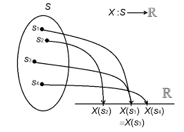
The name random variable suggests a variable that takes on values randomly. In a loose, intuitive way this is the right interpretation – e.g., an observer who is measuring the amount of noise on a communication link sees a random variable in this sense. We require, however, a more precise mathematical definition for analytical purposes. Mathematically a random variable is neither random nor a variable – it is just a function mapping one sample space into another space. The first space is the sample space portion of a probability space, and the second space is a subset of the real line (some authors wotld call this a “real-valued” random variable). The careful mathematical definition will place a constraint on the function to ensure that the theory makes sense, but for the moment we will adopt the informal definition that a random variable is just a function.
A random variable is perhaps best thought of as a measurement on a
probability space; that is, for each sample point $\omega$ the random variable produces some value, denoted functionally as $f(\omega)$. One can view $\omega$ as the result of some experiment and $f(\omega)$ as the restalt of a measurement made on the experiment, as in the example of the simple binary quantizer introduced in the introduction to chapter 2 . The experiment outcome $\omega$ is from an abstract space, e.g., real numbers, integers, ASCII characters, waveforms, sequences, Chinese characters, etc. The resulting value of the measurement or random variable $f(\omega)$, however, must be “concrete” in the sense of being a real number, e.g., a meter reading. The randomness is all in the original probability space and not in the random variable; that is, once the $\omega$ is selected in a “random” way, the output value of sample value of the random variable is determined.
Alternatively, the original point $\omega$ can be viewed as an “input signal” and the random variable $f$ can be viewed as “signal processing,” i.e., the input signal $\omega$ is converted into an “output signal” $f(\omega)$ by the random variable. This viewpoint becomes both precise and relevant when we indeed choose our original sample space to be a signal space and we generalize random variables by random vectors and processes.
Before proceeding to the formal definition of random variables, vectors, and processes, we motivate several of the basic ideas by simple examples, beginning with random variables constructed on the fair wheel experiment of the introduction to chapter 2 .
统计代写|随机信号处理作业代写Statistical Signal Processing代考|A Coin Flip
We have already encountered an example of a random variable in the introduction to chapter 2 , where we defined a random variable $q$ on the spinning wheel experiment which produced an output with the same pmf as a uniform coin flip. We begin by summarizing the idea with some slight notational changes and then consider the implications in additional detail.
Begin with a probability space $(\Omega, \mathcal{F}, P)$ where $\Omega=\Re$ and the probability $P$ is defined by (2.2) using the uniform pdf on $[0,1)$ of (2.4) Define the function $Y: \Re \rightarrow{0,1}$ by
$$
Y(r)= \begin{cases}0 & \text { if } r \leq 0.5 \ 1 & \text { otherwise }\end{cases}
$$
When Tyche performs the experiment of spinning the pointer, we do not actually observe the pointer, but only the resulting binary value of $Y$. $Y$ can be thought of as signal processing or as a measurement on the original experiment. Subject to a technical constraint to be introduced later, any function defined on the sample space of an experiment is called a random
variable. The “randomness” of a random variable is “inherited” from the underlying experiment and in theory the probability measure describing its outputs should be derivable from the initial probability space and the structure of the function. To avoid confusion with the probability measure $P$ of the original experiment, refer to the probability measure associated with outcomes of $Y$ as $P_{Y} . P_{Y}$ is called the distribution of the random variable $Y$. The probability $P_{Y}(F)$ can be defined in a natural way as the probability computed using $P$ of all the original samples that are mapped by $Y$ into the subset $F$ :
$$
P_{Y}(F)=P({r: Y(r) \in F})
$$
统计代写|随机信号处理作业代写Statistical Signal Processing代考|Random Vectors
The issue of the possible equality of two random variables raises an interesting point. If you are told that $Y$ and $V$ are two separate random variables with pm’t’s $p_{Y}$ and $p_{V}$, then the quegtion of whether or not they are equivalent can be answered from these pmf’s alone. If you wish to determine whether or not the two random variables are in fact equal, however, then they must be considered together or jointly. In the case where we have a random variable $Y$ with outcomes in ${0,1}$ and a random variable $V$ with outcomes in ${0,1}$, we could consider the two together as a single random vector ${Y, V}$ with outcomes in the Cartesian product space $\Omega_{Y V}={0,1}^{2} \triangleq{(0,0),(0,1),(1,0),(1,1)}$ with some pmf $p_{Y, V}$ describing the combined behavior
$$
p_{Y, V}(y, v)=\operatorname{Pr}(Y=y, V=v)
$$
so that
$$
\operatorname{Pr}((Y, V) \in F)=\sum_{y, v:(y, v) \in F} p_{Y, V}(y, v) ; F \in \mathcal{B}{Y V}, $$ where in this simple discrete problem we take the event space $\mathcal{B}{Y V}$ to be the power set of $\Omega_{Y V}$. Now the question of equality makes sense as we can evaluate the probability that the two are equal:
$$
\operatorname{Pr}(Y=V)=\sum_{y, v \in Y-v} p_{Y, V}(y, v) .
$$
If this probability is 1 , then we know that the two random variables are in fact equal with probability $1 .$

信号处理代写
统计代写|随机信号处理作业代写Statistical Signal Processing代考|Random Variables
随机变量的名称暗示了一个随机取值的变量。以一种松散、直观的方式,这是正确的解释——例如,测量通信链路上的噪声量的观察者在这个意义上看到了一个随机变量。然而,为了分析的目的,我们需要一个更精确的数学定义。从数学上讲,随机变量既不是随机变量也不是变量——它只是一个将一个样本空间映射到另一个空间的函数。第一个空间是概率空间的样本空间部分,第二个空间是实线的子集(一些作者称其为“实值”随机变量)。仔细的数学定义将对函数施加约束,以确保理论有意义,
随机变量也许最好被认为是对
概率空间;也就是说,对于每个样本点ω随机变量产生一些值,在功能上表示为F(ω). 一个可以查看ω作为一些实验的结果和F(ω)作为对实验进行测量的重新设置,如第 2 章介绍中介绍的简单二进制量化器的示例。实验结果ω来自抽象空间,例如实数、整数、ASCII字符、波形、序列、汉字等。测量或随机变量的结果值F(ω)然而,在实数的意义上,它必须是“具体的”,例如,仪表读数。随机性都在原始概率空间中,而不是在随机变量中;也就是说,一旦ω以“随机”的方式选择,确定随机变量的样本值的输出值。
或者,原点ω可以看作是“输入信号”和随机变量F可以看作是“信号处理”,即输入信号ω转换成“输出信号”F(ω)由随机变量。当我们确实选择我们的原始样本空间作为信号空间并且我们通过随机向量和过程来概括随机变量时,这个观点变得既精确又相关。
在开始正式定义随机变量、向量和过程之前,我们通过简单的例子来激发几个基本的想法,从第 2 章引言的公平轮实验中构建的随机变量开始。
统计代写|随机信号处理作业代写Statistical Signal Processing代考|A Coin Flip
我们已经在第 2 章的介绍中遇到了一个随机变量的例子,我们在其中定义了一个随机变量。q在旋转轮实验中,该实验产生的输出与均匀抛硬币具有相同的 pmf。我们首先通过一些细微的符号变化来总结这个想法,然后更详细地考虑其含义。
从概率空间开始(Ω,F,磷)在哪里Ω=ℜ和概率磷由 (2.2) 使用统一的 pdf 定义[0,1)(2.4)定义函数是:ℜ→0,1经过
是(r)={0 如果 r≤0.5 1 除此以外
当 Tyche 进行旋转指针的实验时,我们实际上并没有观察到指针,而只是观察到的二进制值是. 是可以认为是信号处理或对原始实验的测量。受限于稍后介绍的技术约束,在实验的样本空间上定义的任何函数都称为随机
多变的。随机变量的“随机性”是从基础实验“继承”的,理论上描述其输出的概率度量应该可以从初始概率空间和函数结构推导出来。避免与概率测度混淆磷原始实验的,指的是与结果相关的概率测度是作为磷是.磷是称为随机变量的分布是. 概率磷是(F)可以以自然的方式定义为使用计算的概率磷映射的所有原始样本是进入子集F :
磷是(F)=磷(r:是(r)∈F)
统计代写|随机信号处理作业代写Statistical Signal Processing代考|Random Vectors
两个随机变量可能相等的问题提出了一个有趣的观点。如果你被告知是和在是两个独立的随机变量,带有 pm’t’sp是和p在,那么它们是否等效的问题可以仅从这些 pmf 中回答。但是,如果您希望确定两个随机变量实际上是否相等,则必须将它们一起或共同考虑。在我们有一个随机变量的情况下是结果在0,1和一个随机变量在结果在0,1,我们可以将两者一起视为单个随机向量是,在在笛卡尔积空间中产生结果Ω是在=0,12≜(0,0),(0,1),(1,0),(1,1)有一些 pmfp是,在描述组合行为
p是,在(是,在)=公关(是=是,在=在)
以便
公关((是,在)∈F)=∑是,在:(是,在)∈Fp是,在(是,在);F∈乙是在,在这个简单的离散问题中,我们采用事件空间乙是在成为的幂集Ω是在. 现在相等的问题是有道理的,因为我们可以评估两者相等的概率:
公关(是=在)=∑是,在∈是−在p是,在(是,在).
如果这个概率是 1 ,那么我们知道这两个随机变量实际上是概率相等的1.

统计代写请认准statistics-lab™. statistics-lab™为您的留学生涯保驾护航。
金融工程代写
金融工程是使用数学技术来解决金融问题。金融工程使用计算机科学、统计学、经济学和应用数学领域的工具和知识来解决当前的金融问题,以及设计新的和创新的金融产品。
非参数统计代写
非参数统计指的是一种统计方法,其中不假设数据来自于由少数参数决定的规定模型;这种模型的例子包括正态分布模型和线性回归模型。
广义线性模型代考
广义线性模型(GLM)归属统计学领域,是一种应用灵活的线性回归模型。该模型允许因变量的偏差分布有除了正态分布之外的其它分布。
术语 广义线性模型(GLM)通常是指给定连续和/或分类预测因素的连续响应变量的常规线性回归模型。它包括多元线性回归,以及方差分析和方差分析(仅含固定效应)。
有限元方法代写
有限元方法(FEM)是一种流行的方法,用于数值解决工程和数学建模中出现的微分方程。典型的问题领域包括结构分析、传热、流体流动、质量运输和电磁势等传统领域。
有限元是一种通用的数值方法,用于解决两个或三个空间变量的偏微分方程(即一些边界值问题)。为了解决一个问题,有限元将一个大系统细分为更小、更简单的部分,称为有限元。这是通过在空间维度上的特定空间离散化来实现的,它是通过构建对象的网格来实现的:用于求解的数值域,它有有限数量的点。边界值问题的有限元方法表述最终导致一个代数方程组。该方法在域上对未知函数进行逼近。[1] 然后将模拟这些有限元的简单方程组合成一个更大的方程系统,以模拟整个问题。然后,有限元通过变化微积分使相关的误差函数最小化来逼近一个解决方案。
tatistics-lab作为专业的留学生服务机构,多年来已为美国、英国、加拿大、澳洲等留学热门地的学生提供专业的学术服务,包括但不限于Essay代写,Assignment代写,Dissertation代写,Report代写,小组作业代写,Proposal代写,Paper代写,Presentation代写,计算机作业代写,论文修改和润色,网课代做,exam代考等等。写作范围涵盖高中,本科,研究生等海外留学全阶段,辐射金融,经济学,会计学,审计学,管理学等全球99%专业科目。写作团队既有专业英语母语作者,也有海外名校硕博留学生,每位写作老师都拥有过硬的语言能力,专业的学科背景和学术写作经验。我们承诺100%原创,100%专业,100%准时,100%满意。
随机分析代写
随机微积分是数学的一个分支,对随机过程进行操作。它允许为随机过程的积分定义一个关于随机过程的一致的积分理论。这个领域是由日本数学家伊藤清在第二次世界大战期间创建并开始的。
时间序列分析代写
随机过程,是依赖于参数的一组随机变量的全体,参数通常是时间。 随机变量是随机现象的数量表现,其时间序列是一组按照时间发生先后顺序进行排列的数据点序列。通常一组时间序列的时间间隔为一恒定值(如1秒,5分钟,12小时,7天,1年),因此时间序列可以作为离散时间数据进行分析处理。研究时间序列数据的意义在于现实中,往往需要研究某个事物其随时间发展变化的规律。这就需要通过研究该事物过去发展的历史记录,以得到其自身发展的规律。
回归分析代写
多元回归分析渐进(Multiple Regression Analysis Asymptotics)属于计量经济学领域,主要是一种数学上的统计分析方法,可以分析复杂情况下各影响因素的数学关系,在自然科学、社会和经济学等多个领域内应用广泛。
MATLAB代写
MATLAB 是一种用于技术计算的高性能语言。它将计算、可视化和编程集成在一个易于使用的环境中,其中问题和解决方案以熟悉的数学符号表示。典型用途包括:数学和计算算法开发建模、仿真和原型制作数据分析、探索和可视化科学和工程图形应用程序开发,包括图形用户界面构建MATLAB 是一个交互式系统,其基本数据元素是一个不需要维度的数组。这使您可以解决许多技术计算问题,尤其是那些具有矩阵和向量公式的问题,而只需用 C 或 Fortran 等标量非交互式语言编写程序所需的时间的一小部分。MATLAB 名称代表矩阵实验室。MATLAB 最初的编写目的是提供对由 LINPACK 和 EISPACK 项目开发的矩阵软件的轻松访问,这两个项目共同代表了矩阵计算软件的最新技术。MATLAB 经过多年的发展,得到了许多用户的投入。在大学环境中,它是数学、工程和科学入门和高级课程的标准教学工具。在工业领域,MATLAB 是高效研究、开发和分析的首选工具。MATLAB 具有一系列称为工具箱的特定于应用程序的解决方案。对于大多数 MATLAB 用户来说非常重要,工具箱允许您学习和应用专业技术。工具箱是 MATLAB 函数(M 文件)的综合集合,可扩展 MATLAB 环境以解决特定类别的问题。可用工具箱的领域包括信号处理、控制系统、神经网络、模糊逻辑、小波、仿真等。