如果你也在 怎样代写随机控制Stochastic Control这个学科遇到相关的难题,请随时右上角联系我们的24/7代写客服。
随机控制或随机最优控制是控制理论的一个子领域,它涉及到观察中或驱动系统演变的噪声中存在的不确定性。
随机控制或随机最优控制是控制理论的一个子领域,它涉及到观察中或驱动系统进化的噪声中存在的不确定性。系统设计者以贝叶斯概率驱动的方式假设,具有已知概率分布的随机噪声会影响状态变量的演变和观察。随机控制的目的是设计受控变量的时间路径,以最小的成本执行所需的控制任务,尽管存在这种噪声,但以某种方式定义。
statistics-lab™ 为您的留学生涯保驾护航 在代写随机控制Stochastic Control方面已经树立了自己的口碑, 保证靠谱, 高质且原创的统计Statistics代写服务。我们的专家在代写随机控制Stochastic Control代写方面经验极为丰富,各种代写随机控制Stochastic Control相关的作业也就用不着说。
我们提供的随机控制Stochastic Control及其相关学科的代写,服务范围广, 其中包括但不限于:
- Statistical Inference 统计推断
- Statistical Computing 统计计算
- Advanced Probability Theory 高等概率论
- Advanced Mathematical Statistics 高等数理统计学
- (Generalized) Linear Models 广义线性模型
- Statistical Machine Learning 统计机器学习
- Longitudinal Data Analysis 纵向数据分析
- Foundations of Data Science 数据科学基础
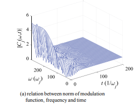
统计代写|随机控制代写Stochastic Control代考|Generalized Probability Density Evolution Equation
Without loss of generality, a stochastic dynamical system under the random excitation can be represented by
$$
\dot{\mathbf{Z}}(t)=\mathbf{g}[\mathbf{Z}(t), \mathbf{F}(\boldsymbol{\Theta}, t), t], \mathbf{Z}\left(t_{0}\right)=\mathbf{z}_{0}
$$
where $\mathbf{F}(\cdot)$ is a column vector denoting the nonstationary and non-Gaussian random excitation; $\boldsymbol{\Theta}$ is a random parameter vector denoting the randomness inherent in the excitation.
As to the quantity of interest such as the system state or the control force $\mathbf{Z}^{\mathrm{T}}=$ $\left{Z_{i}\right}_{i=1}^{m}$, the formal solution can be given by
$$
\mathbf{Z}(t)=\mathbf{H}\left(\boldsymbol{\Theta}, \mathbf{Z}{0}, t\right) $$ where $\mathbf{H}$ is an $m$-dimensional column vector denoting arithmetic operator. It is indicated in Eq. (2.3.61) that the randomness inherent in the random process $\mathbf{Z}(t)$ is completely represented by the random parameter vector $\boldsymbol{\Theta}$. In view of the probability preservation principle, the augmented system consisting of the quantity of interest and the random parameter vector, i.e., $(\mathbf{Z}(t), \mathbf{\Theta})$, thus sustains a preservative probability, that is $$ \frac{\mathrm{D}}{\mathrm{D} t} \int{\Omega_{t} \times \Omega_{\Theta}} p_{\mathbf{Z \Theta}}(\mathbf{z}, \theta, t) \mathrm{d} \mathbf{z} d \theta=0
$$
where $p_{\mathbf{Z} \Theta}(\mathbf{z}, \boldsymbol{\theta}, t)$ denotes the joint probability density function of the augmented system $(\mathbf{Z}(t), \boldsymbol{\Theta}) ; \Omega_{t}$ denotes the time domain; $\Omega_{\boldsymbol{\Theta}}$ denotes the sample domain of random parameter vector $\Theta ; \mathrm{D}(\cdot) / \mathrm{D} t$ denotes the total derivative.
Extending Eq. (2.3.62), we have (Li and Chen 2009)
$\frac{\mathrm{D}}{\mathrm{D} t} \int_{\Omega_{l} \times \Omega_{\boldsymbol{\Theta}}} p_{\mathbf{Z} \Theta}(\mathbf{z}, \boldsymbol{\theta}, t) \mathrm{d} \mathbf{z} \mathrm{d} \theta$
$=\frac{\mathrm{D}}{\mathrm{D} t} \int_{\Omega_{t_{0}} \times \Omega_{\Theta}} p_{\mathbf{Z} \Theta}(\mathbf{z}, \theta, t)|J| \mathrm{d} \mathbf{z} d \theta$
$=\int_{\Omega_{t_{0}} \times \Omega_{\Theta}}\left(|J| \frac{\mathrm{D} p_{\mathbf{Z \Theta}}}{\mathrm{D} t}+p_{\mathbf{Z \Theta}} \frac{\mathrm{D}|J|}{\mathrm{D} t}\right) \mathrm{d} \mathbf{z} d \theta$
$=\int_{\Omega_{t_{0}} \times \bar{\Omega}{\Theta}}\left{|J|\left(\frac{\partial p{\mathbf{Z} \Theta}}{\partial t}+\sum_{j=1}^{m} \dot{Z}{j} \frac{\partial p{\mathbf{Z} \Theta}}{\partial z_{j}}\right)+|J| p_{\mathbf{Z} \Theta} \sum_{j=1}^{m} \frac{\partial \dot{Z}{j}}{\partial z{j}}\right} \mathrm{d} \mathbf{z} d \boldsymbol{\theta}$
统计代写|随机控制代写Stochastic Control代考|Historic Notes
It is generally recognized that the random vibration discipline originates from the research and application of stochastic dynamics that involves two logical clues ( $\mathrm{Li}$ and Chen 2009). Einstein first explored the Brownian motion from a phenomenological perspective using the random process theory in 1905 (Einstein 1905), which was later developed by Fokker (Fokker 1914), Planck (Planck 1917), and mathematized by Kolmogorov (Kolmogorov 1931) that formed into the associated theory and methods with the FPK equation. From an almost coinstantaneous physical perspective, Langevin investigated the motion of a Brownian particle by the Newtonian equation (Langevin 1908), which was later developed by Wiener (Wiener 1923), Itô (Itô 1942) and Stratonovich (Stratonovich 1963) that underlined the formulation and solution schemes of the stochastic differential equation. Although the probabilistic description of structural vibration was pioneered in Rayleigh’s investigation on the random flight in the early of twentieth century (Rayleigh 1919), the random vibration theory was widely applied in the engineering fields and gradually became to a new discipline until the middle of twentieth century. Since then, it has gained extensive progress from the primary linear random vibration analysis such as the random vibration with initial random conditions, the random vibration simultaneously involving the randomness inherent in external excitations and in structural parameters, to the nonlinear random vibration analysis (Crandall 1958; Crandall and Mark 1963; Lin 1967; Nigam 1983; Roberts and Spanos 1990; Lin and Cai 1995; Lutes and Sarkani 2004; Li and Chen 2009).
As to the classical linear random vibration analysis, an elegant theoretical formula and the pertinent numerical schemes have been formed by virtue of the statistical relation between the input and the output in temporal and frequency domains (Crandall 1958), e.g., the spectral transfer matrix method (Lutes and Sarkani 2004), the modal superposition method such as the complete quadratic combination (CQC) (Der Kiureghian 1981; Der Kiureghian and Neuenhofer 1992), the pseudo-excitation method (Lin et al. 2001; Li et al. 2004). However, the principle of superposition is not suitable for the nonlinear system. The temporal and frequency-domain methods prevailing in the linear random vibration analysis cannot deal with the problem of essentially nonlinear random vibrations. The classical Markov process method accommodates a few specific nonlinear systems but encounters the challenge as well in dealing with the general multi-degree-of-freedom and multidimensional systems. It is thus a preferable choice of deriving the approximate solution or the accurate stationary solution for the nonlinear random vibration analysis. In the past over 50 years, a collection of methods for nonlinear random vibration analysis were proposed, e.g., the statistical linearization technique (Caughey 1963) and the moment closure method (Stratonovich 1963) suitable for the weakly nonlinear systems; the extended statistical linearization technique (Beaman and Hedrick 1981), the equivalent nonlinear equation (Caughey 1986), and the Monte Carlo simulation (Shinozuka 1972) suitable for the strongly nonlinear systems. Meanwhile, the attempt of classical stochastic structure theory to the application of random vibration analysis was
carried out. For instance, the perturbation expansion method was applied to deal with the random vibration analysis of low-order systems (Crandall 1963); the orthogonal function expansion was applied to deal with the random vibration analysis of white noise-driven Duffing oscillatory systems (Orabi and Ahmadi 1987); the polynomial chaos expansion was applied to deal with the random vibration analysis of stationary excitation-driven Duffing systems (Li and Ghanem 1998). One might realize that the mentioned methods cannot solve the problem of nonlinear random vibration of highdimensional structural systems, not even to gain the complete probability density. In theory, the FPK equation is the most rigorous and most elegant method for the nonlinear random vibration analysis. As far as steady solution of stochastic dynamical systems is concerned, the method for solving high-dimensional FPK equation in Hamiltonian framework attained systematic progress since 1990 s (Soize 1994; Zhu and Huang 1999; Er 2011). However, when the unsteady solution of stochastic dynamical systems is concerned, the computational complexity will increase exponentially with the dimension of systems. In this case, the solution is still hard to be derived even employing efficiently numerical schemes and advanced computational platforms. In recent years, the dimension reduction of FPK equation has been paid extensive attention (Chen and Yuan 2014; Chen and Rui 2018).
The probability density evolution method (PDEM) with the kernel generalized probability density evolution equation (GDEE) provided an efficient means for solving the stochastic dynamical system from a physical perspective. This method has been applied into the stochastic response analysis and reliability assessment of general nonlinear stochastic systems (Li and Chen 2004a, b, 2005, 2006a; Chen and Li 2005 ; Li and Chen 2008). The progress underlies the development of the physically based stochastic optimal control of structures.
统计代写|随机控制代写Stochastic Control代考|Dynamic Reliability of Structures
The primary goal of structural analysis aims at the performance-based design and control of structures. If the random factors involved in the basic physical background are concerned, the logical manner of structural analysis is to carry out the reliabilitybased structural design and control.
As regards the assessment of dynamic reliability of structures as the first-passage failure criterion, the primary methods include the level-crossing process theory, the diffusion process theory and the probability density evolution method. Two families of criteria are usually applied in the probability density evolution method, i.e., the absorbing boundary condition criterion and the equivalent extreme-value event criterion. Herein, the level-crossing process theory and the equivalent extreme-value event criterion-based probability density evolution methở are intrơuucè sincé thé two methods are both widely used in practice.
The level-crossing process theory originated from Rice’s researches on the digital noise process in 1940 s (Rice 1944,1945 ). As to the $b$-level-crossing process, shown in Fig. 2.4, the probability of occurring once upward level-crossing during the time interval $t<\tau \leqslant t+\Delta t$ is given by $$ \begin{aligned} &\operatorname{Pr}\left{N^{+}(t+\Delta t)-N^{+}(t)=1\right} \ &=\operatorname{Pr}{X(t+\Delta t)>b, X(t)b, X(t)$ $b, xb, X(t)b, xb-\dot{x} \Delta t, x<b} p_{X \dot{X}}(x, \dot{x}, t) \mathrm{d} x \mathrm{~d} \dot{x} \
&=\int_{0}^{\infty} \mathrm{d} \dot{x} \int_{b-\dot{x} \Delta t}^{b} p_{X \dot{X}}(x, \dot{x}, t) \mathrm{d} x
\end{aligned}
$$
随机控制代写
统计代写|随机控制代写Stochastic Control代考|Generalized Probability Density Evolution Equation
不失一般性,随机激励下的随机动力系统可以表示为
从˙(吨)=G[从(吨),F(θ,吨),吨],从(吨0)=和0
在哪里F(⋅)是表示非平稳和非高斯随机激励的列向量;θ是一个随机参数向量,表示激励中固有的随机性。
对于系统状态或控制力等感兴趣的数量从吨= \left{Z_{i}\right}_{i=1}^{m}\left{Z_{i}\right}_{i=1}^{m},正式的解决方案可以由
从(吨)=H(θ,从0,吨)在哪里H是一个米表示算术运算符的维列向量。它在方程式中表示。(2.3.61) 随机过程中固有的随机性从(吨)完全由随机参数向量表示θ. 鉴于概率保存原则,由感兴趣量和随机参数向量组成的增广系统,即(从(吨),θ),因此维持一个保存概率,即
DD吨∫Ω吨×Ωθp从θ(和,θ,吨)d和dθ=0
在哪里p从θ(和,θ,吨)表示增强系统的联合概率密度函数(从(吨),θ);Ω吨表示时域;Ωθ表示随机参数向量的样本域θ;D(⋅)/D吨表示总导数。
扩展方程。(2.3.62),我们有 (Li and Chen 2009)
DD吨∫Ωl×Ωθp从θ(和,θ,吨)d和dθ
=DD吨∫Ω吨0×Ωθp从θ(和,θ,吨)|Ĵ|d和dθ
=∫Ω吨0×Ωθ(|Ĵ|Dp从θD吨+p从θD|Ĵ|D吨)d和dθ
=\int_{\Omega_{t_{0}} \times \bar{\Omega}{\Theta}}\left{|J|\left(\frac{\partial p{\mathbf{Z} \Theta}} {\partial t}+\sum_{j=1}^{m} \dot{Z}{j} \frac{\partial p{\mathbf{Z} \Theta}}{\partial z_{j}}\右)+|J| p_{\mathbf{Z} \Theta} \sum_{j=1}^{m} \frac{\partial \dot{Z}{j}}{\partial z{j}}\right} \mathrm{d } \mathbf{z} d \boldsymbol{\theta}=\int_{\Omega_{t_{0}} \times \bar{\Omega}{\Theta}}\left{|J|\left(\frac{\partial p{\mathbf{Z} \Theta}} {\partial t}+\sum_{j=1}^{m} \dot{Z}{j} \frac{\partial p{\mathbf{Z} \Theta}}{\partial z_{j}}\右)+|J| p_{\mathbf{Z} \Theta} \sum_{j=1}^{m} \frac{\partial \dot{Z}{j}}{\partial z{j}}\right} \mathrm{d } \mathbf{z} d \boldsymbol{\theta}
统计代写|随机控制代写Stochastic Control代考|Historic Notes
人们普遍认为,随机振动学科起源于对随机动力学的研究和应用,涉及到两个逻辑线索(大号一世和陈 2009)。爱因斯坦在 1905 年(Einstein 1905)首次使用随机过程理论从现象学的角度探索了布朗运动,该理论后来由 Fokker(Fokker 1914)、Planck(Planck 1917)发展,并由 Kolmogorov(Kolmogorov 1931)数学化,形成FPK方程的相关理论和方法。从几乎同时发生的物理角度,朗之万通过牛顿方程 (Langevin 1908) 研究了布朗粒子的运动,该方程后来由 Wiener (Wiener 1923)、Itô (Itô 1942) 和 Stratonovich (Stratonovich 1963) 开发,强调了该公式和随机微分方程的解方案。虽然结构振动的概率描述在二十世纪初瑞利对随机飞行的研究中开创了先河(Rayleigh 1919),但随机振动理论在工程领域得到了广泛的应用,并逐渐成为一门新学科,直到二十世纪中叶。世纪。从那时起,它从最初的线性随机振动分析(如具有初始随机条件的随机振动、同时涉及外部激励和结构参数中固有随机性的随机振动)到非线性随机振动分析(Crandall 1958)取得了广泛的进展。 ;Crandall 和 Mark 1963;Lin 1967;Nigam 1983;Roberts 和 Spanos 1990;Lin 和 Cai 1995;Lutes 和 Sarkani 2004;Li 和 Chen 2009)。随机振动理论在工程领域得到广泛应用,直到二十世纪中叶才逐渐成为一门新学科。从那时起,它从最初的线性随机振动分析(如具有初始随机条件的随机振动、同时涉及外部激励和结构参数中固有随机性的随机振动)到非线性随机振动分析(Crandall 1958)取得了广泛的进展。 ;Crandall 和 Mark 1963;Lin 1967;Nigam 1983;Roberts 和 Spanos 1990;Lin 和 Cai 1995;Lutes 和 Sarkani 2004;Li 和 Chen 2009)。随机振动理论在工程领域得到广泛应用,直到二十世纪中叶才逐渐成为一门新学科。从那时起,它从最初的线性随机振动分析(如具有初始随机条件的随机振动、同时涉及外部激励和结构参数中固有随机性的随机振动)到非线性随机振动分析(Crandall 1958)取得了广泛的进展。 ;Crandall 和 Mark 1963;Lin 1967;Nigam 1983;Roberts 和 Spanos 1990;Lin 和 Cai 1995;Lutes 和 Sarkani 2004;Li 和 Chen 2009)。
对于经典的线性随机振动分析,利用输入和输出在时域和频域上的统计关系(Crandall 1958),例如谱传递矩阵法,形成了一个优雅的理论公式和相关的数值方案。 (Lutes and Sarkani 2004)、模态叠加法如完全二次组合 (CQC) (Der Kiureghian 1981; Der Kiureghian and Neuenhofer 1992)、伪励磁法 (Lin et al. 2001; Li et al. 2004) . 但是,叠加原理不适用于非线性系统。线性随机振动分析中流行的时域和频域方法无法处理本质上非线性随机振动的问题。经典的马尔可夫过程方法适用于一些特定的非线性系统,但在处理一般的多自由度和多维系统时也遇到了挑战。因此,对于非线性随机振动分析,推导近似解或精确平稳解是一种优选的选择。在过去的 50 多年里,提出了一系列非线性随机振动分析方法,例如适用于弱非线性系统的统计线性化技术(Caughey 1963)和矩闭合法(Stratonovich 1963);适用于强非线性系统的扩展统计线性化技术(Beaman 和 Hedrick 1981)、等效非线性方程(Caughey 1986)和蒙特卡罗模拟(Shinozuka 1972)。同时,
执行。例如,微扰展开法被用于处理低阶系统的随机振动分析(Crandall 1963);应用正交函数展开来处理白噪声驱动的 Duffing 振荡系统的随机振动分析(Orabi 和 Ahmadi 1987);多项式混沌展开被应用于处理静止激励驱动的 Duffing 系统的随机振动分析 (Li and Ghanem 1998)。人们可能会意识到,上述方法无法解决高维结构系统的非线性随机振动问题,甚至无法获得完整的概率密度。从理论上讲,FPK方程是非线性随机振动分析中最严谨、最优雅的方法。就随机动力系统的稳定解而言,自 1990 年代以来,哈密顿框架中高维 FPK 方程的求解方法取得了系统性进展(Soize 1994;Zhu 和 Huang 1999;Er 2011)。然而,当考虑随机动力系统的非定常解时,计算复杂度会随着系统的维数呈指数增长。在这种情况下,即使采用有效的数值方案和先进的计算平台,仍然很难得出解决方案。近年来,FPK方程的降维得到了广泛的关注(Chen and Yuan 2014; Chen and Rui 2018)。计算复杂度将随着系统的维数呈指数增长。在这种情况下,即使采用有效的数值方案和先进的计算平台,仍然很难得出解决方案。近年来,FPK方程的降维得到了广泛的关注(Chen and Yuan 2014; Chen and Rui 2018)。计算复杂度将随着系统的维数呈指数增长。在这种情况下,即使采用有效的数值方案和先进的计算平台,仍然很难得出解决方案。近年来,FPK方程的降维得到了广泛的关注(Chen and Yuan 2014; Chen and Rui 2018)。
带有核广义概率密度演化方程(GDEE)的概率密度演化方法(PDEM)为从物理角度求解随机动力系统提供了一种有效的手段。该方法已应用于一般非线性随机系统的随机响应分析和可靠性评估(Li and Chen 2004a, b, 2005, 2006a; Chen and Li 2005; Li and Chen 2008)。这一进展是基于物理的结构随机最优控制发展的基础。
统计代写|随机控制代写Stochastic Control代考|Dynamic Reliability of Structures
结构分析的主要目标是基于性能的结构设计和控制。如果考虑到基本物理背景中涉及的随机因素,结构分析的逻辑方式是进行基于可靠性的结构设计和控制。
将结构动力可靠性评估作为首过破坏准则的方法主要有平交过程理论、扩散过程理论和概率密度演化法。概率密度演化法中通常应用两类准则,即吸收边界条件准则和等效极值事件准则。在这里,水平交叉过程理论和基于等效极值事件准则的概率密度演化方法是很深入的,因为这两种方法都在实践中得到了广泛的应用。
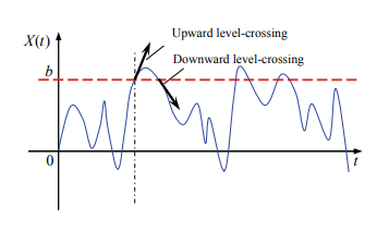
水平交叉过程理论起源于Rice 在1940 年代对数字噪声过程的研究(Rice 1944,1945)。至于b-平交过程,如图2.4所示,时间间隔内发生一次向上平交的概率吨<τ⩽吨+Δ吨是(谁)给的
\begin{aligned} &\operatorname{Pr}\left{N^{+}(t+\Delta t)-N^{+}(t)=1\right} \ &=\operatorname{Pr}{X( t+\Delta t)>b, X(t)b, X(t)$ $b, xb, X(t)b, xb-\dot{x} \Delta t, x<b} p_{X \dot {X}}(x, \dot{x}, t) \mathrm{d} x \mathrm{~d} \dot{x} \ &=\int_{0}^{\infty} \mathrm{d} \dot{x} \int_{b-\dot{x} \Delta t}^{b} p_{X \dot{X}}(x, \dot{x}, t) \mathrm{d} x \结束{对齐}\begin{aligned} &\operatorname{Pr}\left{N^{+}(t+\Delta t)-N^{+}(t)=1\right} \ &=\operatorname{Pr}{X( t+\Delta t)>b, X(t)b, X(t)$ $b, xb, X(t)b, xb-\dot{x} \Delta t, x<b} p_{X \dot {X}}(x, \dot{x}, t) \mathrm{d} x \mathrm{~d} \dot{x} \ &=\int_{0}^{\infty} \mathrm{d} \dot{x} \int_{b-\dot{x} \Delta t}^{b} p_{X \dot{X}}(x, \dot{x}, t) \mathrm{d} x \结束{对齐}

统计代写请认准statistics-lab™. statistics-lab™为您的留学生涯保驾护航。
金融工程代写
金融工程是使用数学技术来解决金融问题。金融工程使用计算机科学、统计学、经济学和应用数学领域的工具和知识来解决当前的金融问题,以及设计新的和创新的金融产品。
非参数统计代写
非参数统计指的是一种统计方法,其中不假设数据来自于由少数参数决定的规定模型;这种模型的例子包括正态分布模型和线性回归模型。
广义线性模型代考
广义线性模型(GLM)归属统计学领域,是一种应用灵活的线性回归模型。该模型允许因变量的偏差分布有除了正态分布之外的其它分布。
术语 广义线性模型(GLM)通常是指给定连续和/或分类预测因素的连续响应变量的常规线性回归模型。它包括多元线性回归,以及方差分析和方差分析(仅含固定效应)。
有限元方法代写
有限元方法(FEM)是一种流行的方法,用于数值解决工程和数学建模中出现的微分方程。典型的问题领域包括结构分析、传热、流体流动、质量运输和电磁势等传统领域。
有限元是一种通用的数值方法,用于解决两个或三个空间变量的偏微分方程(即一些边界值问题)。为了解决一个问题,有限元将一个大系统细分为更小、更简单的部分,称为有限元。这是通过在空间维度上的特定空间离散化来实现的,它是通过构建对象的网格来实现的:用于求解的数值域,它有有限数量的点。边界值问题的有限元方法表述最终导致一个代数方程组。该方法在域上对未知函数进行逼近。[1] 然后将模拟这些有限元的简单方程组合成一个更大的方程系统,以模拟整个问题。然后,有限元通过变化微积分使相关的误差函数最小化来逼近一个解决方案。
tatistics-lab作为专业的留学生服务机构,多年来已为美国、英国、加拿大、澳洲等留学热门地的学生提供专业的学术服务,包括但不限于Essay代写,Assignment代写,Dissertation代写,Report代写,小组作业代写,Proposal代写,Paper代写,Presentation代写,计算机作业代写,论文修改和润色,网课代做,exam代考等等。写作范围涵盖高中,本科,研究生等海外留学全阶段,辐射金融,经济学,会计学,审计学,管理学等全球99%专业科目。写作团队既有专业英语母语作者,也有海外名校硕博留学生,每位写作老师都拥有过硬的语言能力,专业的学科背景和学术写作经验。我们承诺100%原创,100%专业,100%准时,100%满意。
随机分析代写
随机微积分是数学的一个分支,对随机过程进行操作。它允许为随机过程的积分定义一个关于随机过程的一致的积分理论。这个领域是由日本数学家伊藤清在第二次世界大战期间创建并开始的。
时间序列分析代写
随机过程,是依赖于参数的一组随机变量的全体,参数通常是时间。 随机变量是随机现象的数量表现,其时间序列是一组按照时间发生先后顺序进行排列的数据点序列。通常一组时间序列的时间间隔为一恒定值(如1秒,5分钟,12小时,7天,1年),因此时间序列可以作为离散时间数据进行分析处理。研究时间序列数据的意义在于现实中,往往需要研究某个事物其随时间发展变化的规律。这就需要通过研究该事物过去发展的历史记录,以得到其自身发展的规律。
回归分析代写
多元回归分析渐进(Multiple Regression Analysis Asymptotics)属于计量经济学领域,主要是一种数学上的统计分析方法,可以分析复杂情况下各影响因素的数学关系,在自然科学、社会和经济学等多个领域内应用广泛。
MATLAB代写
MATLAB 是一种用于技术计算的高性能语言。它将计算、可视化和编程集成在一个易于使用的环境中,其中问题和解决方案以熟悉的数学符号表示。典型用途包括:数学和计算算法开发建模、仿真和原型制作数据分析、探索和可视化科学和工程图形应用程序开发,包括图形用户界面构建MATLAB 是一个交互式系统,其基本数据元素是一个不需要维度的数组。这使您可以解决许多技术计算问题,尤其是那些具有矩阵和向量公式的问题,而只需用 C 或 Fortran 等标量非交互式语言编写程序所需的时间的一小部分。MATLAB 名称代表矩阵实验室。MATLAB 最初的编写目的是提供对由 LINPACK 和 EISPACK 项目开发的矩阵软件的轻松访问,这两个项目共同代表了矩阵计算软件的最新技术。MATLAB 经过多年的发展,得到了许多用户的投入。在大学环境中,它是数学、工程和科学入门和高级课程的标准教学工具。在工业领域,MATLAB 是高效研究、开发和分析的首选工具。MATLAB 具有一系列称为工具箱的特定于应用程序的解决方案。对于大多数 MATLAB 用户来说非常重要,工具箱允许您学习和应用专业技术。工具箱是 MATLAB 函数(M 文件)的综合集合,可扩展 MATLAB 环境以解决特定类别的问题。可用工具箱的领域包括信号处理、控制系统、神经网络、模糊逻辑、小波、仿真等。