Introduction to stochastic control, with applications taken from a variety of areas including supply-chain optimization, advertising, finance, dynamic resource allocation, caching, and traditional automatic control. Markov decision processes, optimal policy with full state information for finite-horizon case, infinite-horizon discounted, and average stage cost problems. Bellman value function, value iteration, and policy iteration. Approximate dynamic programming. Linear quadratic stochastic control.
PREREQUISITES
EE365 is the same as MS\&E251, Stochastic Decision Models.
Homework 8 solutions have been posted.
Last year’s final for practice, and the solutions.
As a reminder, you are responsible for all announcements made on the Piazza forum.
Paris’ pre-final office hours: Thursday Jun 5, 11-1 in Packard 107
Sanjay’s pre-final office hours: Friday Jun 6, 2-3:30
Samuel’s pre-final office hours: Friday Jun 6, 8:30pm-10pm in Huang 219
EE365 Stochastic control HELP(EXAM HELP, ONLINE TUTOR)
问题 1.
Lemma 1 Consider $\mathbf{z}j$ a vector with the order of $\mathbf{x}_j$, associated to dynamic behavior of the system and independent of the noise input $\xi_j ;$ and $\left.\beta_j^i\right|{j=1, \ldots, k} ^{i=1, \ldots, l}$ is the normalized degree of activation, a variable defined as in (4) associated to $\mathbf{z}j$. Then, at the limit $$ \lim {k \rightarrow \infty} \frac{1}{k} \sum_{j=1}^k\left[\beta_j^1 \mathbf{z}_j, \ldots, \beta_j^l \mathbf{z}_j\right] \xi_j^T=\mathbf{0} $$
问题 2.
Lemma 2 Under the same conditions as Lemma 1 and $\mathbf{z}j$ independent of the disturbance noise $\eta_j$, then, at the limit $$ \lim {k \rightarrow \infty} \frac{1}{k} \sum_{j=1}^k\left[\beta_j^1 \mathbf{z}_j, \ldots, \beta_j^l \mathbf{z}_j\right] \eta_j=0 $$
问题 3.
Lemma 3 Under the same conditions as Lemma 1, according to (23), at the limit $$ \begin{array}{r} \lim {k \rightarrow \infty} \frac{1}{k} \sum{j=1}^k\left[\beta_j^1 \mathbf{z}j, \ldots, \beta_j^l \mathbf{z}_j\right]\left[\gamma_j^1\left(\mathbf{x}_j+\xi_j\right), \ldots\right. \ \left.\gamma_j^l\left(\mathbf{x}_j+\xi_j\right)\right]^T=\mathbf{C}{\mathbf{z x}} \neq 0 \end{array} $$
问题 4.
Theorem 1 Under suitable conditions outlined from Lemma 1 to 3, the estimation of the parameter vector $\theta$ for the model in (12) is strongly consistent, i.e, at the limit $$ p \cdot \lim \theta=0 $$
Textbooks
• An Introduction to Stochastic Modeling, Fourth Edition by Pinsky and Karlin (freely available through the university library here) • Essentials of Stochastic Processes, Third Edition by Durrett (freely available through the university library here) To reiterate, the textbooks are freely available through the university library. Note that you must be connected to the university Wi-Fi or VPN to access the ebooks from the library links. Furthermore, the library links take some time to populate, so do not be alarmed if the webpage looks bare for a few seconds.
统计代写|随机控制代写Stochastic Control代考|Market Definitions and Arbitrage
As in Chap. 1 we fix an $m$-dimensional Brownian motion $B(t)=\left(B_{1}(t), \ldots, B_{m}(t)\right)^{T}$ and $\ell$ independent compensated jump measures $\tilde{N}(\cdot, \cdot)=\left(\tilde{N}{1}(\cdot, \cdot), \ldots, \tilde{N}{\ell}(\cdot, \cdot)\right)^{T}$. Recall that we have assumed that $E\left[\eta^{2}(t)\right]<\infty$ for all $t \geq 0$. We let $\mathcal{F}{t}^{B}$ be the $\sigma$-algebra generated by $B(s) ; s \leq t$ and we let $\mathcal{F}{t}^{N}$ be the $\sigma$-algebra generated by $N(\mathrm{~d} s, \mathrm{~d} z) ; s \leq t$. And we put $\mathcal{F}{t}=\mathcal{F}{t}^{B} \vee \mathcal{F}{t}^{N}$, the $\sigma$-algebra generated by $\mathcal{F}{t}^{B}$ and $\mathcal{F}{t}^{N}$, and $\mathbb{F}=\left{\mathcal{F}{t}\right}_{t \geq 0}$.
Suppose we have a financial market with the following $n+1$ investment possibilities: (i) A risk free asset, where the unit price $S_{0}(t)$ at time $t$ is given by $$ \begin{aligned} \mathrm{d} S_{0}(t) &=r(t) S_{0}(t) \mathrm{d} t ; \quad t \in[0, T] \ S_{0}(0) &=1 \end{aligned} $$ (ii) $n$ risky assets, where the unit price $S_{i}(t)$ at time $t$ is given by $$ \begin{aligned} &\mathrm{d} S_{i}(t)=\mu_{i}(t) \mathrm{d} t+\sigma_{i}(t) \mathrm{d} B(t)+\int_{\mathbb{R}} \gamma_{i}(t, z) \tilde{N}(\mathrm{~d} t, \mathrm{~d} z) ; \quad t \in[0, T] \ &S_{i}(0) \in \mathbb{R} ; \quad 1 \leq i \leq n \end{aligned} $$
统计代写|随机控制代写Stochastic Control代考|Hedging and Completeness
To make sure that the market has no arbitrage, we assume from now on that there exist predictable processes $\theta_{0}(t) \in \mathbb{R}^{m}$ and $\theta_{1}(t, z) \in \mathbb{R}^{\ell}$ such that $\theta_{1, k} \leq 1 ; 1 \leq k \leq \ell$ and (2.1.17) and (2.1.18) hold. We fix such a pair $\theta=\left(\theta_{0}, \theta_{1}\right)$ and define $Z(t) ; Q$, $\mathrm{d} B_{Q}=\theta_{0}(t) \mathrm{d} t+\mathrm{d} B(t)$ and $\tilde{N}{Q}(\mathrm{~d} t, \mathrm{~d} z)=\theta{1}(\mathrm{~d} z) \mathrm{d} t+\tilde{N}(\mathrm{~d} t, \mathrm{~d} z)$ as in Theorem 1.35. We now introduce the following terminology: Definition $2.7$ (a) A claim (or a $T$-claim) is a lower bounded $\mathcal{F}{T}$-measurable random variable. (b) A claim $F$ is called replicable (or hedgable or attainable) if there exists a portfolio $\varphi \in \mathcal{A}$ and a constant $x \in \mathbb{R}$ such that $$ F=X{x}^{\varphi}(T):=x+\int_{0}^{T} \varphi(s) \mathrm{d} S(s) \quad \text { a.s. } $$ and such that the normalized wealth process $$ \bar{X}{x}^{\varphi}(t):=x+\int{0}^{t} \varphi(s) \mathrm{d} \bar{S}(s) $$ is a $Q$-martingale. (c) The market ${S(t)}_{t \in[0, T]}$ is called $\mathcal{F}_{T}$-complete if every bounded claim is replicable. Otherwise the market is incomplete.
What claims are replicable? When is the market complete? To answer such questions we need the following result: (For simplicity we formulate only the 1dimensional case)
From now on (and throughout the rest of this book) we assume that $$ E\left[\eta^{2}(t)\right]<\infty \text { for all } t \geq 0 $$ This implies that we can choose $R=\infty$ and hence replace $\bar{N}$ by $\tilde{N}$ (see Theorem 1.8).
The geometric Lévy process is an example of a Lévy diffusion, i.e., the solution of an SDF driven hy I .évy processes.
Theorem $1.19$ (Existence and Uniqueness of Solutions of Lévy SDEs) Consider the following Lévy $S D E$ in $\mathbb{R}^{n}: X(0)=x_{0} \in \mathbb{R}^{n}$ and $$ \mathrm{d} X(t)=\alpha(t, X(t)) \mathrm{d} t+\sigma(t, X(t)) \mathrm{d} B(t)+\int_{\mathbb{R}^{n}} \gamma\left(t, X\left(t^{-}\right), z\right) \tilde{N}(\mathrm{~d} t, \mathrm{~d} z) $$ where $\alpha:[0, T] \times \mathbb{R}^{n} \rightarrow \mathbb{R}^{n}, \sigma:[0, T] \times \mathbb{R}^{n} \rightarrow \mathbb{R}^{n \times m}$ and $\gamma:[0, T] \times \mathbb{R}^{n} \times \mathbb{R}^{n} \rightarrow$ $\mathbb{R}^{n \times \ell}$ satisfy the following conditions (At most linear growth) There exists a constant $C_{1}<\infty$ such that $$ |\sigma(t, x)|^{2}+|\alpha(t, x)|^{2}+\int_{\mathbb{R}} \sum_{k=1}^{\ell}\left|\gamma_{k}(t, x, z)\right|^{2} \nu_{k}\left(\mathrm{~d} z_{k}\right) \leq C_{1}\left(1+|x|^{2}\right) $$ for all $x \in \mathbb{R}^{n}$ (Lipschitz continuity) There exists a constant $C_{2}<\infty$ such that $$ \begin{aligned} &|\sigma(t, x)-\sigma(t, y)|^{2}+|\alpha(t, x)-\alpha(t, y)|^{2} \ &\quad+\sum_{k=1}^{\ell} \int_{\mathbb{R}}\left|\gamma^{(k)}\left(t, x, z_{k}\right)-\gamma^{(k)}\left(t, y, z_{k}\right)\right|^{2} \nu_{k}\left(\mathrm{~d} z_{k}\right) \leq C_{2}|x-y|^{2}, \end{aligned} $$ for all $x, y \in \mathbb{R}^{n}$.
统计代写|随机控制代写Stochastic Control代考|The Girsanov Theorem and Applications
The Girsanov theorem and the related concept of an equivalent local martingale measure (ELMM) are important in the applications of stochastic analysis to finance.
In this chapter we first give a general semimartingale discussion and then we apply it to Itô-Lévy processes. We refer to [Ka] for more details.
Let $\left(\Omega, \mathcal{F},\left{\mathcal{F}{t}\right}{t \geq 0}, P\right)$ be a filtered probability space. Let $Q$ be another probability measure on $\mathcal{F}{T}$. We say that $Q$ is equivalent to $P \mid \mathcal{F}{T}$ if $P \mid \mathcal{F}{T} \ll Q$ and $Q \ll P \mid \mathcal{F}{T}$, or, equivalently, if $P$ and $Q$ have the same zero sets in $\mathcal{F}{T}$. By the Radon-Nikodym theorem this is the case if and only if we have $$ \mathrm{d} Q(\omega)=Z(T) \mathrm{d} P(\omega) \text { and } \mathrm{d} P(\omega)=Z^{-1}(T) \mathrm{d} Q(\omega) \text { on } \mathcal{F}{T} $$ for some $\mathcal{F}{T}$-measurable random variable $Z(T)>0$ a.s. $P$. In that case we also write $$ \frac{\mathrm{d} Q}{\mathrm{~d} P}=Z(T) \text { and } \frac{\mathrm{d} P}{\mathrm{~d} Q}=Z^{-1}(T) \text { on } \mathcal{F}{T} . $$ We first make a simple, but useful observation. Lemma 1.26 Suppose $Q \ll P$ with $\frac{\mathrm{d} Q}{\mathrm{~d} P}=Z(T)$ on $\mathcal{F}{T}$. Then $$ \begin{gathered} Q\left|\mathcal{F}{t} \ll P\right| \mathcal{F}{t} \text { for all } t \in[0, T] \text { and } \ Z(t):=\frac{\mathrm{d}\left(Q \mid \mathcal{F}{t}\right)}{\mathrm{d}\left(P \mid \mathcal{F}{t}\right)}=E{P}\left[Z(T) \mid \mathcal{F}_{t}\right], \quad 0 \leq t \leq T \end{gathered} $$ In particular, $Z(t)$ is a $P$-martingale.
统计代写|随机控制代写Stochastic Control代考|The Girsanov Theorem and Applications
Girsanov 定理和等效局部鞅测度 (ELMM) 的相关概念在将随机分析应用于金融方面非常重要。 在本章中,我们首先给出一个般性的半鞅讨论,然后我们将其应用于 Itô-Lévy 过程。详情请参阅[Ka]。 $\mathrm{~ 让 ~ l e f t ( \ O m e g a , ~ I m a t h c a l { F } , \ e f t { m a t h c a l { F Y { t } \ r i g h t}$ 测度 $\mathcal{F} T$. 我们说 $Q$ 相当于 $P \mid \mathcal{F} T$ 如果 $P \mid \mathcal{F} T \ll Q$ 和 $Q \ll P \mid \mathcal{F} T$, 或者, 等效地, 如果 $P$ 和 $Q$ 有相同的零集 $\mathcal{F} T$. 根据 Radon-Nikodym 定理,当且仅当我们有 $$ \mathrm{d} Q(\omega)=Z(T) \mathrm{d} P(\omega) \text { and } \mathrm{d} P(\omega)=Z^{-1}(T) \mathrm{d} Q(\omega) \text { on } \mathcal{F} T $$ 对于一些 $\mathcal{F} T$ – 可测量的随机变量 $Z(T)>0$ 作为 $P$. 在这种情况下,我们也写 $$ \frac{\mathrm{d} Q}{\mathrm{~d} P}=Z(T) \text { and } \frac{\mathrm{d} P}{\mathrm{~d} Q}=Z^{-1}(T) \text { on } \mathcal{F} T \text {. } $$ 我们首先做一个简单但有用的观察。 引理 $1.26$ 假设 $Q \ll P$ 和 $\frac{\mathrm{d} Q}{\mathrm{~d} P}=Z(T)$ 上 $\mathcal{F} T$. 然后 $Q|\mathcal{F} t \ll P| \mathcal{F} t$ for all $t \in[0, T]$ and $Z(t):=\frac{\mathrm{d}(Q \mid \mathcal{F} t)}{\mathrm{d}(P \mid \mathcal{F} t)}=E P\left[Z(T) \mid \mathcal{F}_{t}\right], \quad 0 \leq t \leq T$ 尤其是, $Z(t)$ 是一个 $P$-鞅。
统计代写|随机控制代写Stochastic Control代考|Basic Definitions and Results on Lévy Processes
In this chapter we present the basic concepts and results needed for the applied calculus of jump diffusions. Since there are several excellent books which give a detailed account of this basic theory, we will just briefly review it here and refer the reader to these books for more information.
Definition 1.1 Let $\left(\Omega, \mathcal{F}, \mathbb{F}=\left{\mathcal{F}{t}\right}{t \geq 0}, P\right)$ be a filtered probability space. An $\mathbb{F}{t^{-}}$ adapted process ${\eta(t)}{t \geq 0}=\left{\eta_{t}\right}_{t \geq 0} \subset \mathbb{R}$ with $\eta_{0}=0$ a.s. is called a Lévy process if $\eta_{t}$ is continuous in probability and has stationary and independent increments. Theorem 1.2 Let $\left{\eta_{t}\right}$ be a Lévy process. Then $\eta_{t}$ has a càdlàg version (right continuous with left limits) which is also a Lévy process. Proof See, e.g., [P, S]. In view of this result we will from now on assume that the Lévy processes we work with are càdlàg. The jump of $\eta_{t}$ at $t \geq 0$ is defined by $$ \Delta \eta_{t}=\eta_{t}-\eta_{t^{-}} $$ Let $\mathbf{B}{0}$ be the family of Borel sets $U \subset \mathbb{R}$ whose closure $\bar{U}$ does not contain 0 . For $U \in \mathbf{B}{0}$ we define $$ N(t, U)=N(t, U, \omega)=\sum_{s: 0<s \leq t} \mathcal{X}{I I}\left(\Delta \eta{\mathrm{s}}\right) $$ In other words, $N(t, U)$ is the number of jumps of size $\Delta \eta_{s} \in U$ which occur before or at time $t . N(t, U)$ is called the Poisson random measure (or jump measure) of $\eta(\cdot)$
统计代写|随机控制代写Stochastic Control代考|The Itô Formula and Related Results
We now come to the important Itô formula for Itô-Lévy processes: If $X(t)$ is given by (1.1.12) and $f: \mathbb{R}^{2} \rightarrow \mathbb{R}$ is a $C^{2}$ function, is the process $Y(t):=f(t, X(t))$ again an Itô-Lévy process and if so, how do we represent it in the form (1.1.12)?
If we argue heuristically and use our knowledge of the classical Itô formula it is easy to guess what the answer is:
Let $X^{(\mathrm{c})}(t)$ be the continuous part of $X(t)$, i.e., $X^{(\mathrm{c})}(t)$ is obtained by removing the jumps from $X(t)$. Then an increment in $Y(t)$ stems from an increment in $X^{(c)}(t)$ plus the jumps (coming from $N(\cdot, \cdot)$ ). Hence in view of the classical Itô formula we would guess that $$ \begin{aligned} \mathrm{d} Y(t)=& \frac{\partial f}{\partial t}(t, X(t)) \mathrm{d} t+\frac{\partial f}{\partial x}(t, X(t)) \mathrm{d} X^{(\mathrm{c})}(t)+\frac{1}{2} \frac{\partial^{2} f}{\partial x^{2}}(t, X(t)) \cdot \beta^{2}(t) \mathrm{d} t \ &+\int_{\mathbb{R}}\left{f\left(t, X\left(t^{-}\right)+\gamma(t, z)\right)-f\left(t, X\left(t^{-}\right)\right)\right} N(\mathrm{~d} t, \mathrm{~d} z) \end{aligned} $$ It can be proved that our guess is correct. Since $$ \mathrm{d} X^{(\mathrm{c})}(t)=\left(\alpha(t)-\int_{|z|<R} \gamma(t, z) \nu(\mathrm{d} z)\right) \mathrm{d} t+\beta(t) \mathrm{d} B(t) $$ this gives the following result.
统计代写|随机控制代写Stochastic Control代考|Basic Definitions and Results on Lévy Processes
在本章中,我们介绍了跳跃扩散应用微积分所需的基本概念和结果。由于有几本优秀的书籍详细介绍了这一基本理 论,我们将在这里简要回顾一下,并让读者参考这些书籍以获取更多信息。 定义 $1.1 \mathrm{~ 让 ~ V e f t ( \ O m e g a , ~ \ m a t h c a l { F } , ~ \ m a t h b b { F } = I l e f t {}$ 间。一个 $\mathbb{F} t^{-} \mathrm{~ 适 应 过 程 { 㣛 e t a}$ 程,如果 $\eta_{t}$ 在概率上是连续的,并且具有固定且独立的增量。 定理 $1.2$ 让业ft{leta_{t}\right} 是一个 Lévy 过程。然后 $\eta_{t}$ 有一个 càdlàg 版本(右连续与左极限),这也是一个 Lévy 过程。 证明参见例如 $[\mathrm{P}, \mathrm{S}]$ 。 鉴于这个结果,我们从现在开始假设我们使用的 Lévy 过程是 càdlàg。 的跳跃 $\eta_{t}$ 在 $t \geq 0$ 定义为 $$ \Delta \eta_{t}=\eta_{t}-\eta_{t^{-}} $$ 让 $\mathbf{B} 0$ 成为 Borel 集的家族 $U \subset \mathbb{R}$ 谁的关闭 $\bar{U}$ 不包含 0 。为了 $U \in \mathbf{B} 0$ 我们定义 $$ N(t, U)=N(t, U, \omega)=\sum_{s: 0<s \leq t} \mathcal{X} I I(\Delta \eta \mathrm{s}) $$ 换句话说, $N(t, U)$ 是大小的跳跃次数 $\Delta \eta_{s} \in U$ 发生在之前或时间 $t . N(t, U)$ 称为泊松随机测度 (或跳跃测度) $\eta(\cdot)$
统计代写|随机控制代写Stochastic Control代考|The Itô Formula and Related Results
Performance-based design and control of structures not only relies upon the structural model and the computational method but also relies upon the rationality of the modeling of random dynamis excitations of structures. Classical random process theory usually employs the power spectral density to describe the random excitations, such as the Kanai-Tajimi spectrum (Kanai 1957; Tajimi 1960) used in the earthquake engineering community, the Davenport spectrum (Davenport 1961) used in the wind engineering community, and the Pierson-Moskowitz spectrum (Pierson and Moskowiz 1964) used in the marine engineering community. One might recognize that the power spectral density denotes the second-order statistics of stationary processes in essence, which hardly reveals, however, the complete probabilistic information of original random processes. Moreover, the measure on the power spectral density of random excitations cannot be accurately delivered to the stochastic response through nonlinear structural systems, not mentioned to carry out the logical control of structural performance. However, a family of physically motivated random excitation models has been developed in recent years by exploring the physical mechanism of engineering excitations (Li 2006; 2008). For illustrative purposes, the modeling of random seismic ground motion and of spatial fluctuating wind-velocity field are investigated herein, and the pertinent theory and methods are introduced.
It is well understood that the behaviors of seismic ground motions rely upon a series of critical factors such as the fault mechanism, propagation medium, and properties of the local site (Boore 2003). Due to the uncontrollability of these factors, the observed seismic ground motion arises to have a significant randomness. An efficient means for exploring the seismic wave and its propagation is to establish a wave equation with boundary conditions in conjunction with the seismic source motion (Aki and Richards 1980).
统计代写|随机控制代写Stochastic Control代考|Spectral Transfer Function
Assuming that the propagation medium is homogenous, elastic, and timeindependent, the one-dimensional seismic ground motion field is governed by a wave cquation as follows (Wang and Li 2011): $$ \sum_{j=0}^{n} \sum_{k=0}^{m} a_{j k} \frac{\partial^{j+k}}{\partial x^{j} \partial t^{k}} u(x, t)=0 $$
where $a_{j k}$ is a medium-relevant parameter; $u(x, t)$ denotes the wave displacement of seismic ground motion. The initial and boundary conditions are given by $$ u(0, t)=u_{0}(t),\left.\quad \frac{\partial^{i} u(x, t)}{\partial t^{i}}\right|{t \rightarrow 0}=0,\left.\quad \frac{\partial^{i} u(x, t)}{\partial t^{i}}\right|{t \rightarrow+\infty}=0, i=0,1, \ldots, n $$ By virtue of the Fourier transform, the partial differential equation shown in Eq. (2.5.1) can be transformed into an ordinary differential equation, of which the solution has a formulation as follows: $$ U(x, \omega)=\sum_{j=0}^{n} b_{j}(\omega) \exp \left(-\mathrm{i} k_{j}(\omega) x\right) $$ where $k_{j}(\omega)$ is the eigenvalue of wave displacement, which relies upon the propagation medium; $b_{j}(\omega)$ denotes the synthetic effect of seismic source and propagation path. Inverse Fourier transform on the wave displacement $U(x, \omega)$, yields $$ u(x, t)=\frac{1}{2 \pi} \sum_{j=0}^{n} \int_{-\infty}^{\infty} B_{j}(\omega, x) \exp \left[\mathrm{i} \omega\left(t-\frac{x}{c_{j}(\omega)}\right)\right] \mathrm{d} \omega $$ where $c_{j}(\omega)=\omega / \operatorname{Re}\left[k_{j}(\omega)\right] ; \operatorname{Re}[\cdot]$ denotes real component. Equation (2.5.4) can be further expanded as $$ \begin{aligned} u(x, t)=& \frac{1}{2 \pi} \int_{-\infty}^{\infty} A\left(b_{0}(\omega), \ldots, b_{n}(\omega) ; k_{0}(\omega), \ldots, k_{n}(\omega) ; \omega, x\right) \ & \cdot \cos \left[\omega t+\Phi\left(b_{0}(\omega), \ldots, b_{n}(\omega) ; k_{0}(\omega), \ldots, k_{n}(\omega) ; \omega, x\right)\right] \mathrm{d} \omega \end{aligned} $$ It is indicated that the seismic ground motion field can be represented as a formulation of superposition harmonics, of which the amplitude and phase both are influenced by the boundary condition and the characteristics of propagation medium. Assuming that the specific engineering site is far from the seismic source and the fault develops extensively fast, the dislocation process of seismic source can be viewed as irrelevance with the behaviors of the propagation path of seismic wave. Meanwhile, the scale of the local engineering site is far less than that of the propagation path of seismic wave, and the frequeney seatter effect of local site on the seismic ground motion can be ignored safely. The amplitude spectrum $A(\omega, x)$ and the phase angle $\Phi(\omega, x)$ in Eq. (2.5.5) can be thus written in a separation formulation (Wang and Li 2011).
统计代写|随机控制代写Stochastic Control代考|Seismic Source Model
Seismic source models in seismology are mainly classified into the kinematic models and dynamic models (Aki and Richards 1980). The former describes the kinematic characteristics of seismic source and focuses on the modeling of motion amplitude of seismic source. The latter describes the dynamic characteristics of seismic source and focuscs on the modeling of dislocation and dynamic devclopment of scismic source. The kinematic model of seismic source is widely used in the earthquake engineering community. The most celebrated spectral models pertaining to the kinematics of seismic source are the $\omega^{-3}$ model based on the Haskell rectangular dislocation mechanism of seismic source (Haskell 1964,1966 ), the $\omega^{-2}$ model based on the
Haskell rectangular dislocation mechanism of seismic source (Aki 1967), and the Brune source model based on the Brune circle dislocation mechanism of seismic source (Brune 1970). Among these models, the Brune source model has the benefits of less parameters and solid physical background, in which the fault surface is assumed to be circular and the dislocation distributes uniformly on the fault surface, and the shear stress wave caused by the shear stress drop propagates perpendicular to the dislocation surface. The Fourier amplitude spectrum and the Fourier phase spectrum on the Brune source model are thus denoted as follows (Brune 1970): $$ A_{s}\left(\alpha_{E}, \omega\right)=\frac{A_{0}}{\omega \sqrt{\omega^{2}+\left(\frac{1}{\tau}\right)^{2}}}, \Phi_{s}\left(\alpha_{E}, \omega\right)=\arctan \left(\frac{1}{\omega \tau}\right) $$ where $\alpha_{E}=\left(A_{0}, \tau\right)$ denotes the random vector of physical parameters relevant to the seismic source; $A_{0}$ denotes the amplitude parameter which is a random variable pertaining to intensity of seismic source; $\tau$ denotes the source parameter which is a random variable pertaining to the characteristics of seismic source.
统计代写|随机控制代写Stochastic Control代考| Modeling of Random Dynamic Excitations
在(X,吨)=12圆周率∫−∞∞一种(b0(ω),…,bn(ω);ķ0(ω),…,ķn(ω);ω,X) ⋅因[ω吨+披(b0(ω),…,bn(ω);ķ0(ω),…,ķn(ω);ω,X)]dω 表明地震动场可以表示为叠加谐波的公式,其幅度和相位都受边界条件和传播介质特性的影响。 假设具体工程地点远离震源且断层广泛快速发育,则震源错位过程可以看作与地震波传播路径的行为无关。同时,当地工程场地的规模远小于地震波的传播路径,当地场地对地震动的频率座效应可以忽略不计。幅度谱一种(ω,X)和相位角披(ω,X)在等式。因此,(2.5.5)可以写成分离公式(Wang and Li 2011)。
统计代写|随机控制代写Stochastic Control代考|Seismic Source Model
地震学中的震源模型主要分为运动模型和动力模型(Aki and Richards 1980)。前者描述了震源的运动学特性,侧重于震源运动幅度的建模。后者描述了震源的动力学特征,重点讨论了震源的位错和动态演化建模。震源运动学模型在地震工程界得到广泛应用。与震源运动学有关的最著名的谱模型是ω−3基于震源的Haskell矩形位错机制的模型(Haskell 1964,1966),ω−2模型基于
统计代写|随机控制代写Stochastic Control代考|Generalized Probability Density Evolution Equation
统计代写|随机控制代写Stochastic Control代考|Generalized Probability Density Evolution Equation
Without loss of generality, a stochastic dynamical system under the random excitation can be represented by $$ \dot{\mathbf{Z}}(t)=\mathbf{g}[\mathbf{Z}(t), \mathbf{F}(\boldsymbol{\Theta}, t), t], \mathbf{Z}\left(t_{0}\right)=\mathbf{z}_{0} $$ where $\mathbf{F}(\cdot)$ is a column vector denoting the nonstationary and non-Gaussian random excitation; $\boldsymbol{\Theta}$ is a random parameter vector denoting the randomness inherent in the excitation.
As to the quantity of interest such as the system state or the control force $\mathbf{Z}^{\mathrm{T}}=$ $\left{Z_{i}\right}_{i=1}^{m}$, the formal solution can be given by $$ \mathbf{Z}(t)=\mathbf{H}\left(\boldsymbol{\Theta}, \mathbf{Z}{0}, t\right) $$ where $\mathbf{H}$ is an $m$-dimensional column vector denoting arithmetic operator. It is indicated in Eq. (2.3.61) that the randomness inherent in the random process $\mathbf{Z}(t)$ is completely represented by the random parameter vector $\boldsymbol{\Theta}$. In view of the probability preservation principle, the augmented system consisting of the quantity of interest and the random parameter vector, i.e., $(\mathbf{Z}(t), \mathbf{\Theta})$, thus sustains a preservative probability, that is $$ \frac{\mathrm{D}}{\mathrm{D} t} \int{\Omega_{t} \times \Omega_{\Theta}} p_{\mathbf{Z \Theta}}(\mathbf{z}, \theta, t) \mathrm{d} \mathbf{z} d \theta=0 $$ where $p_{\mathbf{Z} \Theta}(\mathbf{z}, \boldsymbol{\theta}, t)$ denotes the joint probability density function of the augmented system $(\mathbf{Z}(t), \boldsymbol{\Theta}) ; \Omega_{t}$ denotes the time domain; $\Omega_{\boldsymbol{\Theta}}$ denotes the sample domain of random parameter vector $\Theta ; \mathrm{D}(\cdot) / \mathrm{D} t$ denotes the total derivative. Extending Eq. (2.3.62), we have (Li and Chen 2009) $\frac{\mathrm{D}}{\mathrm{D} t} \int_{\Omega_{l} \times \Omega_{\boldsymbol{\Theta}}} p_{\mathbf{Z} \Theta}(\mathbf{z}, \boldsymbol{\theta}, t) \mathrm{d} \mathbf{z} \mathrm{d} \theta$ $=\frac{\mathrm{D}}{\mathrm{D} t} \int_{\Omega_{t_{0}} \times \Omega_{\Theta}} p_{\mathbf{Z} \Theta}(\mathbf{z}, \theta, t)|J| \mathrm{d} \mathbf{z} d \theta$ $=\int_{\Omega_{t_{0}} \times \Omega_{\Theta}}\left(|J| \frac{\mathrm{D} p_{\mathbf{Z \Theta}}}{\mathrm{D} t}+p_{\mathbf{Z \Theta}} \frac{\mathrm{D}|J|}{\mathrm{D} t}\right) \mathrm{d} \mathbf{z} d \theta$ $=\int_{\Omega_{t_{0}} \times \bar{\Omega}{\Theta}}\left{|J|\left(\frac{\partial p{\mathbf{Z} \Theta}}{\partial t}+\sum_{j=1}^{m} \dot{Z}{j} \frac{\partial p{\mathbf{Z} \Theta}}{\partial z_{j}}\right)+|J| p_{\mathbf{Z} \Theta} \sum_{j=1}^{m} \frac{\partial \dot{Z}{j}}{\partial z{j}}\right} \mathrm{d} \mathbf{z} d \boldsymbol{\theta}$
统计代写|随机控制代写Stochastic Control代考|Historic Notes
It is generally recognized that the random vibration discipline originates from the research and application of stochastic dynamics that involves two logical clues ( $\mathrm{Li}$ and Chen 2009). Einstein first explored the Brownian motion from a phenomenological perspective using the random process theory in 1905 (Einstein 1905), which was later developed by Fokker (Fokker 1914), Planck (Planck 1917), and mathematized by Kolmogorov (Kolmogorov 1931) that formed into the associated theory and methods with the FPK equation. From an almost coinstantaneous physical perspective, Langevin investigated the motion of a Brownian particle by the Newtonian equation (Langevin 1908), which was later developed by Wiener (Wiener 1923), Itô (Itô 1942) and Stratonovich (Stratonovich 1963) that underlined the formulation and solution schemes of the stochastic differential equation. Although the probabilistic description of structural vibration was pioneered in Rayleigh’s investigation on the random flight in the early of twentieth century (Rayleigh 1919), the random vibration theory was widely applied in the engineering fields and gradually became to a new discipline until the middle of twentieth century. Since then, it has gained extensive progress from the primary linear random vibration analysis such as the random vibration with initial random conditions, the random vibration simultaneously involving the randomness inherent in external excitations and in structural parameters, to the nonlinear random vibration analysis (Crandall 1958; Crandall and Mark 1963; Lin 1967; Nigam 1983; Roberts and Spanos 1990; Lin and Cai 1995; Lutes and Sarkani 2004; Li and Chen 2009).
As to the classical linear random vibration analysis, an elegant theoretical formula and the pertinent numerical schemes have been formed by virtue of the statistical relation between the input and the output in temporal and frequency domains (Crandall 1958), e.g., the spectral transfer matrix method (Lutes and Sarkani 2004), the modal superposition method such as the complete quadratic combination (CQC) (Der Kiureghian 1981; Der Kiureghian and Neuenhofer 1992), the pseudo-excitation method (Lin et al. 2001; Li et al. 2004). However, the principle of superposition is not suitable for the nonlinear system. The temporal and frequency-domain methods prevailing in the linear random vibration analysis cannot deal with the problem of essentially nonlinear random vibrations. The classical Markov process method accommodates a few specific nonlinear systems but encounters the challenge as well in dealing with the general multi-degree-of-freedom and multidimensional systems. It is thus a preferable choice of deriving the approximate solution or the accurate stationary solution for the nonlinear random vibration analysis. In the past over 50 years, a collection of methods for nonlinear random vibration analysis were proposed, e.g., the statistical linearization technique (Caughey 1963) and the moment closure method (Stratonovich 1963) suitable for the weakly nonlinear systems; the extended statistical linearization technique (Beaman and Hedrick 1981), the equivalent nonlinear equation (Caughey 1986), and the Monte Carlo simulation (Shinozuka 1972) suitable for the strongly nonlinear systems. Meanwhile, the attempt of classical stochastic structure theory to the application of random vibration analysis was
carried out. For instance, the perturbation expansion method was applied to deal with the random vibration analysis of low-order systems (Crandall 1963); the orthogonal function expansion was applied to deal with the random vibration analysis of white noise-driven Duffing oscillatory systems (Orabi and Ahmadi 1987); the polynomial chaos expansion was applied to deal with the random vibration analysis of stationary excitation-driven Duffing systems (Li and Ghanem 1998). One might realize that the mentioned methods cannot solve the problem of nonlinear random vibration of highdimensional structural systems, not even to gain the complete probability density. In theory, the FPK equation is the most rigorous and most elegant method for the nonlinear random vibration analysis. As far as steady solution of stochastic dynamical systems is concerned, the method for solving high-dimensional FPK equation in Hamiltonian framework attained systematic progress since 1990 s (Soize 1994; Zhu and Huang 1999; Er 2011). However, when the unsteady solution of stochastic dynamical systems is concerned, the computational complexity will increase exponentially with the dimension of systems. In this case, the solution is still hard to be derived even employing efficiently numerical schemes and advanced computational platforms. In recent years, the dimension reduction of FPK equation has been paid extensive attention (Chen and Yuan 2014; Chen and Rui 2018).
The probability density evolution method (PDEM) with the kernel generalized probability density evolution equation (GDEE) provided an efficient means for solving the stochastic dynamical system from a physical perspective. This method has been applied into the stochastic response analysis and reliability assessment of general nonlinear stochastic systems (Li and Chen 2004a, b, 2005, 2006a; Chen and Li 2005 ; Li and Chen 2008). The progress underlies the development of the physically based stochastic optimal control of structures.
统计代写|随机控制代写Stochastic Control代考|Dynamic Reliability of Structures
The primary goal of structural analysis aims at the performance-based design and control of structures. If the random factors involved in the basic physical background are concerned, the logical manner of structural analysis is to carry out the reliabilitybased structural design and control.
As regards the assessment of dynamic reliability of structures as the first-passage failure criterion, the primary methods include the level-crossing process theory, the diffusion process theory and the probability density evolution method. Two families of criteria are usually applied in the probability density evolution method, i.e., the absorbing boundary condition criterion and the equivalent extreme-value event criterion. Herein, the level-crossing process theory and the equivalent extreme-value event criterion-based probability density evolution methở are intrơuucè sincé thé two methods are both widely used in practice.
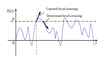
The level-crossing process theory originated from Rice’s researches on the digital noise process in 1940 s (Rice 1944,1945 ). As to the $b$-level-crossing process, shown in Fig. 2.4, the probability of occurring once upward level-crossing during the time interval $t<\tau \leqslant t+\Delta t$ is given by $$ \begin{aligned} &\operatorname{Pr}\left{N^{+}(t+\Delta t)-N^{+}(t)=1\right} \ &=\operatorname{Pr}{X(t+\Delta t)>b, X(t)b, X(t)$ $b, xb, X(t)b, xb-\dot{x} \Delta t, x<b} p_{X \dot{X}}(x, \dot{x}, t) \mathrm{d} x \mathrm{~d} \dot{x} \ &=\int_{0}^{\infty} \mathrm{d} \dot{x} \int_{b-\dot{x} \Delta t}^{b} p_{X \dot{X}}(x, \dot{x}, t) \mathrm{d} x \end{aligned} $$
统计代写|随机控制代写Stochastic Control代考|Generalized Probability Density Evolution Equation
对于经典的线性随机振动分析,利用输入和输出在时域和频域上的统计关系(Crandall 1958),例如谱传递矩阵法,形成了一个优雅的理论公式和相关的数值方案。 (Lutes and Sarkani 2004)、模态叠加法如完全二次组合 (CQC) (Der Kiureghian 1981; Der Kiureghian and Neuenhofer 1992)、伪励磁法 (Lin et al. 2001; Li et al. 2004) . 但是,叠加原理不适用于非线性系统。线性随机振动分析中流行的时域和频域方法无法处理本质上非线性随机振动的问题。经典的马尔可夫过程方法适用于一些特定的非线性系统,但在处理一般的多自由度和多维系统时也遇到了挑战。因此,对于非线性随机振动分析,推导近似解或精确平稳解是一种优选的选择。在过去的 50 多年里,提出了一系列非线性随机振动分析方法,例如适用于弱非线性系统的统计线性化技术(Caughey 1963)和矩闭合法(Stratonovich 1963);适用于强非线性系统的扩展统计线性化技术(Beaman 和 Hedrick 1981)、等效非线性方程(Caughey 1986)和蒙特卡罗模拟(Shinozuka 1972)。同时,
执行。例如,微扰展开法被用于处理低阶系统的随机振动分析(Crandall 1963);应用正交函数展开来处理白噪声驱动的 Duffing 振荡系统的随机振动分析(Orabi 和 Ahmadi 1987);多项式混沌展开被应用于处理静止激励驱动的 Duffing 系统的随机振动分析 (Li and Ghanem 1998)。人们可能会意识到,上述方法无法解决高维结构系统的非线性随机振动问题,甚至无法获得完整的概率密度。从理论上讲,FPK方程是非线性随机振动分析中最严谨、最优雅的方法。就随机动力系统的稳定解而言,自 1990 年代以来,哈密顿框架中高维 FPK 方程的求解方法取得了系统性进展(Soize 1994;Zhu 和 Huang 1999;Er 2011)。然而,当考虑随机动力系统的非定常解时,计算复杂度会随着系统的维数呈指数增长。在这种情况下,即使采用有效的数值方案和先进的计算平台,仍然很难得出解决方案。近年来,FPK方程的降维得到了广泛的关注(Chen and Yuan 2014; Chen and Rui 2018)。计算复杂度将随着系统的维数呈指数增长。在这种情况下,即使采用有效的数值方案和先进的计算平台,仍然很难得出解决方案。近年来,FPK方程的降维得到了广泛的关注(Chen and Yuan 2014; Chen and Rui 2018)。计算复杂度将随着系统的维数呈指数增长。在这种情况下,即使采用有效的数值方案和先进的计算平台,仍然很难得出解决方案。近年来,FPK方程的降维得到了广泛的关注(Chen and Yuan 2014; Chen and Rui 2018)。
带有核广义概率密度演化方程(GDEE)的概率密度演化方法(PDEM)为从物理角度求解随机动力系统提供了一种有效的手段。该方法已应用于一般非线性随机系统的随机响应分析和可靠性评估(Li and Chen 2004a, b, 2005, 2006a; Chen and Li 2005; Li and Chen 2008)。这一进展是基于物理的结构随机最优控制发展的基础。
统计代写|随机控制代写Stochastic Control代考|Dynamic Reliability of Structures
The solution of Eq. (2.3.35) can be represented by a truncated polynomial chaos expansion (PCE) (Ghanem and Spanos 1991), i.e., $$ x_{i}(t)=\sum_{l=0}^{P} x_{i l}(t) \Psi_{l}(\xi) $$ where $\xi$ is the $M$-dimensional row vector of Gaussian random variables; $P$ denotes the highest order of the polynomial chaos expansion; $\Psi_{l}(\xi)$ denotes the polynomial chaos with parameter of Gaussian random variables; $x_{i l}(t)$ denotes the deterministic coefficient pertaining to the polynomial chaos which is often referred to as the random mode. Substituting Eq. (2.3.37) into Eq. (2.3.35), then yields $$ \begin{aligned} &\sum_{i=1}^{n} \sum_{l=0}^{P} m_{j i} \ddot{x}{i l}(t) \Psi{l}(\xi)+\sum_{i=1}^{n} \sum_{k=0}^{q} \alpha_{j i, k}\left(\sum_{l=0}^{P} \dot{x}{i l}(t) \Psi{l}(\xi)\right)^{q-k}\left(\sum_{l=0}^{P} x_{i l}(t) \Psi_{l}(\xi)\right)^{k} \ &\quad=\sum_{l=0}^{P} F_{j l}(t) \Psi_{l}(\xi) \end{aligned} $$ Introducing a Galerkin projection technique (Ghanem and Spanos 1991), the polynomial chaos arises to pairwise orthogonal with respect to Gaussian measure, i.e., $$ \left\langle\Psi_{i} \Psi_{j}\right\rangle=\left\langle\Psi_{i}^{2}\right\rangle \delta_{i j} $$ where $\langle\cdot\rangle$ denotes the inner product; $\delta_{i j}$ denotes the Kronecker delta function with two variables, which is 1 if the variables are equal, and 0 otherwise: $$ \delta_{i j}=\left{\begin{array}{l} 1, i=j \ 0, i \neq j \end{array}\right. $$ Equation (2.3.38) is thus discretized into an equation set:
$$ \begin{aligned} &\sum_{i=1}^{n} m_{j i} \ddot{x}{i m}(t)+\sum{i=1}^{n} \sum_{k=0}^{q} \sum_{l_{1}=0}^{P} \cdots \sum_{l_{q-l}=0}^{P} \sum_{l_{q-k+1}=0}^{P} \cdots \sum_{l_{q}=0}^{P} \frac{c_{l_{1} \cdots l_{q-\lambda} l_{q-\lambda+1} \cdots l_{q} m}}{\left(\Psi_{m}^{2}\right)} \ &\alpha_{j i, k} \dot{x}{i l{1}}(t) \cdots \dot{x}{i l{q-k}}(t) x_{i l_{q-k+1}}(t) \cdots x_{i l_{q}}(t)=F_{j m}(t) \end{aligned} $$ where $c_{l_{1} \cdots l_{q-k} l_{q-k+1} \cdots l_{q} m}=\left\langle\Psi_{l_{1}} \ldots \Psi_{l_{q-k}} \Psi_{l_{q-k+1}} \ldots \Psi_{l_{q}} \Psi_{m}\right\rangle, m=0,1,2, \ldots, P$. The coefficient $c_{l_{1} \cdots l_{4-k} l_{4-k+1} \cdots l_{q} m}$ and $\left\langle\Psi_{m}^{2}\right\rangle$ can be derived from a multiple-dimensional integral (Ghanem and Spanos 1991).
An alternative method for random vibration analysis of nonlinear systems is the statistical linearization technique (Roberts and Spanos 1990). This method exhibits
a hypothesis that the structural response is viewed as a stationary Gaussian process, thereby the equivalence between the linearized system and the original nonlinear system is attained by minimizing their differences in the sense of mean square. The random vibration analysis of nonlinear systems can then be carried out by the pertinent theory and methods to the random vibration of linear systems.
Therefore, the nonlinear multiple-degree-of-freedom system, shown in Eq. (2.3.34), can be substituted by a linearized system with equation of motion as follows: $$ \mathbf{M} \ddot{\mathbf{X}}(t)+\mathbf{C}{\mathrm{eq}} \dot{\mathbf{X}}(t)+\mathbf{K}{\mathrm{eq}} \mathbf{X}(t)=\mathbf{F}(\boldsymbol{\Theta}, t) $$ where $\mathbf{C}{e q}, \mathbf{K}{\text {eq }}$ are the $n \times n$ equivalent damping and equivalent stiffness matrices, respectively.
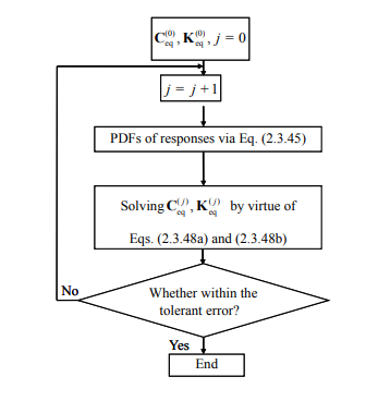
Comparing Eqs. (2.3.34) and (2.3.45), and assuming that the linearized system and the original system have a same response, one can define the error vector between the internal forces of the two systems as follows: $$ \mathbf{e}=\mathbf{f}(\mathbf{X}(t), \dot{\mathbf{X}}(t))-\mathbf{C}{\mathrm{eq}} \dot{\mathbf{X}}(t)-\mathbf{K}{\mathrm{eq}} \mathbf{X}(t) $$ Minimization of the covariance matrix of the error vector, i.e., $$ \begin{aligned} &\frac{\partial E\left[\mathbf{e e}^{\mathrm{T}}\right]}{\partial \mathbf{C}{\mathrm{eq}}}=0 \ &\frac{\partial E\left[\mathbf{e}^{\mathrm{T}}\right]}{\partial \mathbf{K}{\mathrm{eq}}}=0 \end{aligned} $$ yields the basic equations: $$ \begin{aligned} &\mathbf{C}{\mathrm{eq}} E\left[\dot{\mathbf{X}} \dot{\mathbf{X}}^{\mathrm{T}}\right]+\mathbf{K}{\mathrm{eq}} E\left[\mathbf{X} \dot{\mathbf{X}}^{\mathrm{T}}\right]=E\left[\mathbf{f}(\mathbf{X}, \dot{\mathbf{X}}) \dot{\mathbf{X}}^{\mathrm{T}}\right] \ &\mathbf{C}{\mathrm{eq}} E\left[\dot{\mathbf{X}} \mathbf{X}^{\mathrm{T}}\right]+\mathbf{K}{\mathrm{eq}} E\left[\mathbf{X} \mathbf{X}^{\mathrm{T}}\right]=E\left[\mathbf{f}(\mathbf{X}, \dot{\mathbf{X}}) \mathbf{X}^{\mathrm{T}}\right] \end{aligned} $$ Given the joint probability density functions for solving the mathematical expectation of responses, shown in Eqs. (2.3.48a) and (2.3.48b), the equivalent damping and equivalent stiffness matrices can be readily attained. This treatment, however, often refers to an iteration procedure, as shown in Fig. 2.3, where the tolerant error can be set as the difference of response vectors or as the norm of the difference of mean-square response vectors between the sequential steps.
As to a single-degree-of-freedom system, the basic equations with respect to the equivalent damping and equivalent stiffness matrices are given as follows: $$ C_{\mathrm{eq}} E\left[\dot{X}^{2}\right]+K_{\mathrm{eq}} E[X \dot{X}]=E[f(X, \dot{X}) \dot{X}] $$
The mean-square solution of system response under random vibration just includes the former two-order moments information of stochastic dynamical systems, which is insufficient to represent the stochastic response as a complete probabilistic density function, especially for the nonlinear system, of which the probabilistic distribution is distinguished from the normal distribution. Therefore, seeking for the probability density of stochastic dynamical system has received extensive attention. Owing to the contributions from Fokker, Planck, and Kolmogorov, the probability density evolution equation related to random excitations were established in 1930 s. This is the celebrated Fokker-Planck-Kolmogorov equation, i.e., FPK equation, in the classical random vibration theory.
Considering a random process $\mathbf{Z}(t)$, one has the Itô stochastic differential equation as follows: $$ \mathrm{d} \mathbf{Z}(t)=\mathbf{A}(\mathbf{Z}, t) \mathrm{d} t+\mathbf{B}(\mathbf{Z}, t) \mathrm{d} \mathbf{w}(t) $$ As for a random function $f(\mathbf{Z})$ in terms of random process $\mathbf{Z}(t)$, the Taylor series expansion is given by $$ \begin{aligned} \mathrm{d} f(\mathbf{Z}) &=\sum_{i=1}^{m} \frac{\partial f}{\partial z_{i}} \mathrm{~d} z_{i}+\frac{1}{2} \sum_{i=1}^{m} \sum_{j=1}^{m} \frac{\partial^{2} f}{\partial z_{i} \partial z_{j}} \mathrm{~d} z_{i} \mathrm{~d} z_{j}+\cdots \ &=\sum_{i=1}^{m} \frac{\partial f}{\partial z_{i}}\left[A_{i} \mathrm{~d} t+\sum_{k=1}^{r} B_{i k} \mathrm{~d} w_{k}(t)\right]+\frac{1}{2} \sum_{i=1}^{m} \sum_{j=1}^{m}\left[\frac{\partial^{2} f}{\partial z_{i} \partial z_{j}} \sum_{k=1}^{r} B_{i k} \mathrm{~d} w_{k}(t) \sum_{s=1}^{r} B_{j s} \mathrm{~d} w_{s}(t)\right]+\cdots \end{aligned} $$ Taking mathematical expectation on both sides of Eq. (2.3.53), and utilizing the product $E\left[(\mathrm{~d} w(t))^{2}\right]=W \mathrm{~d} t$, the Taylor series expansion has a truncated formulation with respect to $\mathrm{d} t$ : $$ E[\mathrm{~d} f(\mathbf{Z})]=E\left{\left[\sum_{i=1}^{m} A_{i} \frac{\partial f}{\partial z_{i}}+\frac{1}{2} \sum_{i=1}^{m} \sum_{j=1}^{m}\left(\mathbf{B} \mathbf{W B}^{\mathrm{T}}\right){i j} \frac{\partial^{2} f}{\partial z{i} \partial z_{j}}\right] \mathrm{d} t\right} $$ where $\mathbf{W}(t)$ is the $s \times s$ symmetric, and semi-positive spectral density matrix, shown in Eq. (2.2.4). It is noted as well $E\left[\mathrm{~d} w_{k}(t)\right]=0$.
Noting the conditional probability density of $\mathbf{Z}(t)$ as $\tilde{p}{\mathbf{Z}}\left(\mathbf{z}, t \mid \mathbf{z}{0}, t_{0}\right)$, the derivative of left side of Eq.
In practical applications, the complexity of attaining the analytical solution of the unit impulse response function $\mathbf{h}(t)$ is far more than that of the frequency response transfer function $\mathbf{H}(\omega)$ for a multiple-degree-of-freedom system. Moreover, the solution procedure of mean-square responses often involves high-dimensional integrals on the unit impulse response function and on the frequency response transfer function. The computational cost is unacceptable in most cases. In fact, for the linear stochastic dynamical system, a workload-reduced way refers to the so-called modal superposition method. The basic idea is that the original multiple-degree-of-freedom
stochastic system is decoupled into a series of single-degree-of-freedom stochastic systems, so as to significantly reduce the computational cost.
According to the principle of the modal superposition method, the equation of motion of the stochastic dynamical system shown in Eq. (2.3.1) can be rewritten as $$ \overline{\mathbf{M}} \ddot{\mathbf{U}}(t)+\overline{\mathbf{C}} \dot{\mathbf{U}}(t)+\overline{\mathbf{K}} \mathbf{U}(t)=\boldsymbol{\Phi}^{\mathrm{T}} \mathbf{F}(\boldsymbol{\Theta}, t) $$ where $\overline{\mathbf{M}}=\boldsymbol{\Phi}^{\mathrm{T}} \mathbf{M} \boldsymbol{\Phi}, \overline{\mathbf{C}}=\boldsymbol{\Phi}^{\mathrm{T}} \mathbf{C} \boldsymbol{\Phi}, \overline{\mathbf{K}}=\boldsymbol{\Phi}^{\mathrm{T}} \mathbf{K} \boldsymbol{\Phi}$ are the $n \times n$ modal mass, modal damping, and modal stiffness matrices, respectively; $\mathbf{U}=\boldsymbol{\Phi}^{\mathrm{T}} \mathbf{X}$ is the $n$-dimensional column vector denoting modal displacement; $\boldsymbol{\Phi}=\left[\phi_{1}, \phi_{2}, \ldots, \phi_{q}\right]=\left[\phi_{i j}\right]_{n \times q}$ $(q \leq n)$ is the modal matrix.
Assuming that the damping matrix $\mathbf{C}$ is a proportional damping matrix, Eq. (2.3.14) can be then decomposed into $q$ mutually independent single-degreeof-freedom systems, of which the equation of motion of the $j$ th-order mode is shown as follows: $$ \ddot{u}{i}(t)+2 \zeta{i} \omega_{i} \dot{u}{i}(t)+\omega{j}^{2} u_{i}(t)=\frac{1}{\bar{m}{j}} \phi{j}^{\mathrm{T}} \mathbf{F}(\boldsymbol{\Theta}, t)=\frac{1}{\bar{m}{j}} \sum{k=1}^{n} \phi_{i k} F_{k}(\boldsymbol{\Theta}, t), j=1,2, \ldots, q $$ where $\bar{m}{j}$ is the $j$ th-order modal mass; $\omega{j}$ is the $j$ th-order modal frequency; $\zeta_{j}$ is the $j$ th-order modal damping ratio.
By means of the Duhamel integral, the componental formulation of the displacement of the linear system in the modal space can be derived as $$ u_{j}(t)=\frac{1}{\bar{m}{j}} \int{0}^{t} h_{j}(t-\tau) \phi_{j}^{\mathrm{T}} \mathbf{F}(\boldsymbol{\Theta}, \tau) \mathrm{d} \tau $$ where $u_{j}(t)$ is referred to as the $j$ th-order modal displacement. The displacement solution of the linear system in the original state space is then given by $$ \mathbf{X}(t)=\sum_{j=1}^{q} \frac{1}{\bar{m}{j}} \int{0}^{t} h_{j}(t-\tau) \phi_{j} \phi_{j}^{\mathrm{T}} \mathbf{F}(\boldsymbol{\Theta}, \tau) \mathrm{d} \tau $$ Further, the mean and correlation function of the displacement can be deduced as follows: $$ \mu_{\mathbf{X}}(t)=E[\mathbf{X}(t)]=\sum_{j=1}^{q} \frac{1}{\bar{m}{j}} \int{0}^{t} h_{j}(t-\tau) \phi_{j} \phi_{j}^{\mathrm{T}} \mu_{\mathbf{F}}(\tau) \mathrm{d} \tau $$
When the linear system exhibits a high dimension, solving the power spectral density (PSD) of the system response shown in Eq. (2.3.27) involves a complicated procedure. The pseudo-excitation method (PEM) could be employed to obtain the PSD solution in an elegant manner (Lin et al. 2001). This method decomposes the solving procedure into a series of deterministic harmonic analysis through constructing a
pseudo-harmonic excitation. This treatment can enhance the efficiency of numerical schemes significantly.
Denoting the PSD of the random excitation $\mathbf{F}(\boldsymbol{\Theta}, t)$ as $\mathbf{S}{\mathbf{F}}(\omega)$, a pseudo-harmonic excitation $\mathbf{F}=\widetilde{\mathbf{F}}{\sqrt{\mathbf{s}}} \mathrm{e}^{\mathrm{i} \omega t}$ can be readily constructed, where $\widetilde{\mathbf{F}}{\sqrt{\mathbf{s}}}$ satisfies $\widetilde{\mathbf{F}}{\sqrt{\mathbf{s}}} \cdot \widetilde{\mathbf{F}}{\sqrt{\mathbf{s}}}^{*}=$ $\mathbf{S}{\mathbf{F}}(\omega)$, i denotes the imaginary unit. Replacing the excitation in Eq. (2.3.14) by the pseudo-excitation yields $$ \overline{\mathbf{M}} \tilde{\mathbf{U}}(t)+\overline{\mathbf{C}} \tilde{\mathbf{U}}(t)+\overline{\mathbf{K}} \tilde{\mathbf{U}}(t)=\mathbf{F}^{\mathrm{T}} \tilde{\mathbf{F}}_{\sqrt{\mathbf{s}}} \mathrm{e}^{\mathrm{i} \omega t} $$ where $\tilde{\tilde{U}}(t), \tilde{\mathbf{U}}(t), \tilde{\mathbf{U}}(t)$ are the $n$-dimensional column vectors denoting the corresponding acceleration, velocity, and displacement to the system subjected to the pseudo-excitation, respectively.
According to the classical random vibration theory, the stationary solution of Eq. (2.3.28) can be deduced as $$ \tilde{U}{j}(\omega, t)=\frac{1}{\bar{m}{j}} H_{j}(\omega) \phi_{j}^{\mathrm{T}} \tilde{\mathbf{F}}{\sqrt{\mathbf{s}}} \mathrm{e}^{\mathrm{i} \omega t} $$ The auto-power spectral density of system response is then derived as follows: $$ \begin{aligned} S{U_{j}} \widetilde{U}{k}(\omega) &=\widetilde{U}{j}(\omega, t) \widetilde{U}{k}^{*}(\omega, t)=\frac{1}{\bar{m}{j} \bar{m}{k}} H{j}(\omega) H_{k}(\omega) \phi_{j}^{\mathrm{T}} \widetilde{\mathbf{F}}{\sqrt{\mathbf{s}}} \widetilde{\mathbf{F}}{\sqrt{\mathbf{s}}} \phi_{k} \ &=\frac{1}{\bar{m}{j} \bar{m}{k}} H_{j}(\omega) H_{k}(\omega) \phi_{j}^{\mathrm{T}} \mathbf{S}{\mathbf{F}}(\omega) \phi{k}=S_{U_{j} U_{k}}(\omega) \end{aligned} $$ It is shown that in the calculation of spectral density function, the factor of pseudoharmonic excitation $\mathrm{e}^{\mathrm{i} \omega t}$ is always paired with its complex conjugate $\mathrm{e}^{-\mathrm{i} \omega t}$ which are eventually counteracted by multiplication, revealing the time-independent behaviors of auto- and cross-power spectral densities of stationary processes. Further, one can attain the mean-square solution of system responses: $$ E\left[\mathbf{U}(t) \mathbf{U}^{\mathrm{T}}(t)\right]=\frac{1}{2 \pi} \int_{-\infty}^{\infty} \mathbf{S}{\mathbf{U}}(\omega) \mathrm{d} \omega $$ Projecting the generalized coordinate space onto the original coordinate space, then $$ E\left[\mathbf{X}(t) \mathbf{X}^{\mathrm{T}}(t)\right]=\boldsymbol{\Phi} E\left[\mathbf{U}(t) \mathbf{U}^{\mathrm{T}}(t)\right] \boldsymbol{\Phi}^{\mathrm{T}}=\frac{1}{2 \pi} \int{-\infty}^{\infty} \boldsymbol{\Phi} \mathbf{S}_{\mathbf{U}}(\omega) \boldsymbol{\Phi}^{\mathrm{T}} \mathrm{d} \omega $$
统计代写|随机控制代写Stochastic Control代考|Nonlinear Random Vibration
Without loss of generality, a nonlinear stochastic dynamical system is investigated, of which the equation of motion is given by $$ \mathbf{M} \ddot{\mathbf{X}}(t)+\mathbf{f}(\mathbf{X}(t), \dot{\mathbf{X}}(t))=\mathbf{F}(\boldsymbol{\Theta}, t) $$ where $\mathbf{f}(\cdot)$ is the $n$-dimensional column vector denoting nonlinear internal force. The nonlinear internal force is assumed to be denoted by a polynomial function of velocity and displacement. In fact, this is a weak hypothesis, and a large family of dynamical systems can be represented by the formulation, such as the Duffing oscillator with nonlinear stiffness force and the van der Pol oscillator with coupling nonlinearities between stiffness and damping forces. The componental form of the equation is then written as $$ \sum_{i=1}^{n} m_{j i} \ddot{x}{i}(t)+\sum{i=1}^{n} \sum_{k=0}^{q} \alpha_{j i, k} \dot{x}{i}^{q-k}(t) x{i}^{k}(t)=F_{j}(\boldsymbol{\Theta}, t) $$ where $j=1,2, \ldots, n, m_{j i}$ denotes the element of mass matrix; $\ddot{x}{i}(t), \dot{x}{i}(t), x_{i}(t)$ denote the acceleration, velocity, and displacement pertaining to the $i$ th component, respectively; $q$ denotes the highest order of the polynomial function of the internal
force; $\alpha_{j i, k}$ denotes the coefficient of the polynomial function. As the highest order $q$ is set as 1, Eq. (2.3.35) is reduced to a linear formulation: $$ \sum_{i=1}^{n} m_{j i} \ddot{x}{i}(t)+\sum{i=1}^{n} \alpha_{j i, 0} \dot{x}{i}(t)+\sum{i=1}^{n} \alpha_{j i, 1} x_{i}(t)=F_{j}(\Theta, t) $$ where $\alpha_{j i, 0}, \alpha_{j i, 1}$ denote the coefficients relevant to damping force and the restoring force, respectively.
统计代写|随机控制代写Stochastic Control代考|Random Vibration of Structures
统计代写|随机控制代写Stochastic Control代考|Nonlinear Random Vibration
不失一般性,研究了一个非线性随机动力系统,其运动方程为
米X¨(吨)+F(X(吨),X˙(吨))=F(θ,吨) 在哪里F(⋅)是个n维列向量表示非线性内力。 假设非线性内力由速度和位移的多项式函数表示。事实上,这是一个弱假设,并且可以用该公式表示一大类动力系统,例如具有非线性刚度力的 Duffing 振子和具有刚度和阻尼力之间耦合非线性的 van der Pol 振子。然后方程的分量形式写为
Stochastic optimal control is a subfield of control theory, which focuses upon the stochastic systems and develops into a cross-discipline between the stochastic process theory and the optimal control theory. The associated theories and technologies with the electronics and information engineering, mechanical engineering, and aerospace engineering, were flourished since $1960 \mathrm{~s}$, and just concerned the state adjustment of systems under random disturbances such as random excitations and measurement noise. The development in the field of civil engineering began after the seventies of twentieth century. Different from the requirements of the fields of mechanical engineering and aerospace engineering, the civil engineering structures exhibit a large size and experience a complicated external excitation. They have to encounter a series of challenging issues in regard to the safety, the durability, and the comfortability. These issues become more serious in the case of hazardous actions with uncertainties inherent in the occurring time, occurring space, and occurring intensity. The conventional stochastic optimal control theory, however, originated from the random process theory assumes the white Gaussian noise as the random disturbance, which is obviously far from the hazardous actions of engineering structures. Therefore, it is necessary to explore a logical theory and pertinent methods for the stochastic optimal control of civil engineering structures which circumvents the dilemma encountered by the conventional stochastic optimal control theory.
This chapter aims at addressing the theoretical principles relevant to the succeeding chapters in this book. The remaining sections included in this chapter include the classical stochastic optimal control, the random vibration of structures, and its advances that underlies the solution methods for controlled stochastic dynamical systems, the dynamic reliability of structures that underlies the design basis for probabilistic criteria of stochastic optimal control of structures, and the modeling of random dynamic excitations that underlies the uncertainty quantification and simulation of hazardous actions of engineering structures. Through integrating the involved sections, the principle for the theory and methods of stochastic optimal control of structures are provided.
统计代写|随机控制代写Stochastic Control代考|Classical Stochastic Optimal Control
The stochastic optimal control aims at attaining the optimal control law that promotes the stochastic system to an expected state through minimizing a certain cost function by the celebrated optimal control schemes. It is well recognized that the pioneering work on the optimal control theory is the proposal of calculus of variations. In history, Pierre and Fermat introduced firstly the so-called Fermat’s least action principle to explore the minimum path of ray propagating through the optical media in 1662. In 1755, Lagrange introduced the delta calculus, and then Euler proposed the elementary definition of variation method. In $1930 \mathrm{~s}$, the Hamilton-Jacobi equation was derived in the framework of the variation method owing to Hamilton and Jacobi’s contributions. Till the mid-twentieth century, the classical variation theory was completely established. The research of modern optimal control theory began from the late period of World War II. Its theoretical milestones consist of the maximum principle proposed by Pontryagin in 1956 , the dynamic programming proposed by Bellman in 1957 , the state-space method, and linear filtering theory developed by Kalman in 1960 (Yong and Zhou 1999). In early of 1960 s, owing to the developments of the stochastic maximum principle (Kushner 1962) and the stochastic dynamic programming (Florentin 1961 ), the research of stochastic optimal control theory was marked as the beginning.
In state space, the equation of motion of a controlled stochastic dynamical system can be written as $$ \dot{\mathbf{Z}}(t)=\mathbf{g}[\mathbf{Z}(t), \mathbf{U}(t), \mathbf{w}(t), t], \mathbf{Z}\left(t_{0}\right)=\mathbf{Z}_{0} $$ The output equation of the system is given by $$ \hat{\mathbf{Z}}(t)=\mathbf{h}[\mathbf{Z}(t), \mathbf{U}(t), \mathbf{w}(t), t] $$ The measure equation of the system is then given by $$ \mathbf{Y}(t)=\mathbf{j}[\hat{\mathbf{Z}}(t), \mathbf{n}(t), t] $$ where $\mathbf{Z}(t)$ is the $2 n$-dimensional column vector denoting system state; $\hat{\mathbf{Z}}(t)$ is the $m$ dimensional vector denoting system output; $\mathbf{U}(t)$ is the $r$-dimensional vector denoting control force; $\mathbf{w}(t)$ is the $s$-dimensional vector denoting random excitations; $\mathbf{n}(t)$ is the $m$-dimensional vector denoting measurement noise; $\mathbf{Y}(t)$ is the $m$-dimensional measured vector denoting system state; $\mathbf{g}(\cdot)$ is the $2 n$-dimensional functional vector denoting system state evolution; $\mathbf{h}(\cdot), \mathbf{j}(\cdot)$ are the $m$-dimensional functional vectors denoting the output and measurement of systems, respectively, which both rely upon the number of sensors.
统计代写|随机控制代写Stochastic Control代考|Spectral Transfer Matrix Method
A linear stochastic dynamical system is considered as follows: $$ \mathbf{M} \ddot{\mathbf{X}}(t)+\mathbf{C} \dot{\mathbf{X}}(t)+\mathbf{K X}(t)=\mathbf{F}(\boldsymbol{\Theta}, t) $$ where $\mathbf{M}, \mathbf{C}$, and $\mathbf{K}$ are the $n \times n$ mass, damping, and stiffness matrices, respectively; $\ddot{\mathbf{X}}(t), \dot{\mathbf{X}}(t), \mathbf{X}(t)$ are the $n$-dimensional column vectors denoting system acceleration, velocity, and displacement, respectively; $\mathbf{F}(\boldsymbol{\Theta}, t)$ is the $n$-dimensional column vector denoting random excitations, and $\boldsymbol{\Theta}$ is an $n_{\boldsymbol{\Theta} \text {-dimensional vector denoting random }}$ parameters of system which exhibits the joint probability density function $p_{\boldsymbol{\Theta}}(\boldsymbol{\theta})$. Defining the $n \times n$ unit impulse response function matrices $\mathbf{h}(t)$, where the component $h_{i j}(t)$ denotes the response of the $i$ th degree in the case that the unit impulse acts on the $j$ th degree of the system, one can attain the system response $\mathbf{h}{j}(t)$ from the equation of motion as follows: $$ \mathbf{M} \ddot{\mathbf{h}}{j}(t)+\mathbf{C} \dot{\mathbf{h}}{j}(t)+\mathbf{K h}{j}(t)=\mathbf{I}{j} \delta(\boldsymbol{\Theta}, t) $$ where $\mathbf{I}{j}=(\underbrace{0,0, \ldots, 0,1}_{j}, 0, \ldots, 0)^{\mathrm{T}}$ is $n$-dimensional column vectors denoting the location of the unit impulse $\delta(\boldsymbol{\Theta}, t)$ acting on the $j$ th degree of the system.
统计代写|随机控制代写Stochastic Control代考|Challenges of Structural Control in Civil Engineering
统计代写|随机控制代写Stochastic Control代考|Challenges of Structural Control in Civil Engineering
The control theory and methods were thrived in the fields of electronics and information engineering, mechanical engineering, aerospace engineering, etc. They focus on the state regulation of systems under distributions such as random excitations and measurement noise, while new challenging issues have to be encountered when these achievements are applied into the field of civil engineering. Different from the practical demands, however, as emerged in the mechanical engineering and aerospace
engineering, there are more uncertainty and higher complexity inherent in civil engineering. The structural control in civil engineering involves a variety of practical challenges such as the structural safety, system durability, structural comfortability, etc. Moreover, large output and high performance are claimed as to the control devices. The challenging issues of structural control in civil engineering that are distinguished from the classical control theory and methods lie in dynamic excitations, structural parameters, nonlinear effects, control law formulas, and control modalities. (i) Challenges related to dynamic excitations In the period of service, the civil engineering structures usually suffer from the dynamic excitations, especially from the risk of hazardous dynamic actions. The hazardous dynamic actions such as strong earthquakes, high winds, and huge waves exhibit significant randomness inherent in their occurring time, occurring space, and occurring intensity. The influences of random excitations upon the accurate quantification of structural state and the logical design of control systems are thus prominent. The classical stochastic optimal control theory, derived from the Itô stochastic differential equation, is restricted to the assumption of white Gaussian noise excitations and measurement noise. It still lacks the sufficient exploration into the case under the general random excitations. This limitation owes to the fact the classical stochastic optimal control theory has been mostly applied in the nonmechanical problems such as those raised from the mechanical engineering and aerospace engineering. While the challenges related to the random excitation become predominant, the stochastic optimal control theory is used to deal with the mechanical problems that occur in the civil engineering. In fact, the seismic ground motion exhibits significant nonstationarities, and the high wind even just the stable airflow exhibits certain nonstationarities. However, the random excitations in the classical stochastic optimal control are almost assumed to be stationary white Gaussian noise, which is obviously far from the hazardous dynamic actions upon the civil engineering structures. (ii) Challenges related to structural parameters Due to the uncertainties inherent in the structural materials and manufactures, the basic parameters of civil engineering structures usually exhibit randomness. This brings about a series of new issues to the structural control. The influences of random parameters upon the stochastic optimal control of structures give rise to two aspects. One is the state estimation. The Kalman filter theory is a celebrated method for dealing with the measurement noise and the incomplete measurement in the classical system control. How this method is applied to state estimation of structures with random parameters constitutes a new challenge. The other is the stability of control system. The presence of random parameters leads to the issue of stochastic eigenvalues, which also brings about a new challenge to the Lyapunov stability theory based stability analysis of classical control systems.
统计代写|随机控制代写Stochastic Control代考|Physically Based Stochastic Optimal Control
It is readily recognized that the relevant theory and methods of classical stochastic optimal control are all developed on the basis of Itô calculus, which underlies the state equation of systems. This treatment allows an exclusive assumption that the external excitation is viewed as a white Gaussian noise or a filtered white Gaussian noise, which is far from the real engineering excitations. This assumption thus limits the engineering application of the classical stochastic optimal control in practice. In fact, the assumption hinders the development of the modern theory of stochastic dynamical system as well. Just in view of this situation, the probability density evolution method was developed based on the probability preservation principle. The PDEM bridges the essential relation between the probability density evolution and the physical state evolution of systems, that is, the physical state evolution of systems drives the probbabbility density evoolution. Thẽ dêtêministic systêm and the stōchāstic system can thus be summarized into a unified framework ( $\mathrm{Li}$ and Chen 2009). Moreover, this progress profoundly reveals that the physical evolution mechanism of systems is still the critical content of stochastic system researches, which underlies the theory of physical stochastic system. In this framework, a novel theory and the associated methods for the stochastic optimal control of structures are expected to develop. In the end nineteenth century, the research of practical systems with random initial state formed the basis of the Gibbs-Liouville theory, and proved the celebrated Liouville equation (Syski 1967). It is Einstein who addressed the special cases of diffusion processes and established the diffusion equation for Brownian motion in 1905 (Einstein 1905). Then it was extended by Fokker and Planck who derived the classical Fokker-Planck equation (Fokker 1914; Planck 1917). In 1931, Kolmogorov independently deduced a same formulation as the Fokker-Planck equation, and a backward Kolmogorov equation was then derived (Kolmogorov 1931). Owing to the rigorous mathematical basis, the Kolmogorov equation is so-called the FokkerPlanck-Kolmogorov equation (FPK equation). Thereafter, the FPK equation and its solutions formed the primary topics of random vibration theory. In 1957, Dostupov and Pugachev attempted to quantify the randomness inherent in the system input through introducing the Karhunen-Loeve decomposition (Dostupov and Pugachev 1957). It is the so-called Dostupov-Pugachev equation. It is regret; however, the equations mentioned above are all high-dimensional and strong-coupling partial differential equations, of which the analytical solutions are hardly derived. Li and Chen explored the probability preservation principle in an elegant manner, and secured the essential relation between probability density evolution and physical state evolution of systems. A family of decoupling probability density evolution equations, i.e., the so-called generalized probability density evolution equation (GDEE), was then proposed in the past 15 years (Li and Chen $2006 \mathrm{a}, \mathrm{b}, \mathrm{c}, 2008,2009$ ). It is recognized that the GDEE accommodates the randomness both inherent in external excitations and in structural systems, which provides a new way to carry out the response analysis and reliability assessment of stochastic systems subjected to general random excitations, and also allows a potential for stochastic optimal control of linear and nonlinear multi-degree-of-freedom systems.
统计代写|随机控制代写Stochastic Control代考|Scope of the Book
In the civil engineering community, the objective of structural control is often definite, while the loads acting on the engineering structures cannot be predicted accurately, especially for the dynamic excitations. Therefore, the stochastic optimal control of structures considering the randomness inherent in engineering excitations ought to be paid sufficient attention. For this reason, the present book focuses on the hazardous dynamic actions, specifically on the random seismic ground motion and the
fluctuating wind-velocity field, and devotes to developing a novel theory and the pertinent successful strategies for stochastic optimal control of engineering structures, in conjunction with the probability density evolution method. The outline is sketched as follows: the performance evolution of controlled systems is first investigated, and a family of probabilistic criteria in terms of structural responses is then established; the generalized optimal control policy and the associated control law involving the simultaneous optimization of the controller parameters and the control device placement are then proposed; in order to verify the propused methodulogy, a scries of engineering applications and experimental studies of controlled structures are then introduced. The scope of the book is illustrated as follows: In Chap. 2, the associated theoretical principles pertaining to the physically based stochastic optimal control are addressed, including the classical stochastic optimal control in the framework of the stochastic maximum principle and the stochastic dynamic programming, the random vibration of linear and nonlinear structures, the dynamic reliability of structures, and the modeling of random dynamic excitations. The kernel equation of the PDEM, i.e., the generalized probability density evolution equation, is introduced as well. This chapter devotes to providing a solid foundation for the successive developments of theory and methods of stochastic optimal control of structures.
In Chap. 3, the probability density evolution method of stochastic optimal control is detailed. Performance evolution of controlled structural systems is first investigated. The solution of the physically based stochastic optimal control is deduced according to Pontryagin’s maximum principle. Active stochastic optimal control based on the probabilistic criterion on system second-order statistics evaluation is discussed. For validating purposes, comparative studies against the classical LQG control are carried out.
In Chap. 4 , a family of probabilistic criteria for the physically based stochastic optimal control is proposed, including the single-objective optimization criteria with respect to the second-order moments such as the mean and the variance, and with respect to the tail of probability density, i.e., the exceedance probability, of equivalent extreme-value responses: and the multiple-objective optimization criteria with respect to the mean and the exceedance probability of equivalent extreme-value responses in performance trade-off and in energy trade-off, respectively. Numerical examples are studied to prove the applicability of the proposed probabilistic criteria. In Chap. 5, the concept of generalized optimal control policy is proposed. This concept indicates a unified formula of the optimal control law with optimized controller parameters pertaining to passive, active, semiactive, and hybrid controls, and with optimized control device placement. In order to attain the optimal placement of control devices at each sequential step, a probabilistic controllability index in argument of exceedance probability is defined. Comparative studies between control device deployment strategies using the minimum controllability index gradient criterion and the maximum controllability index criterion are then carried out.
统计代写|随机控制代写Stochastic Control代考|Challenges of Structural Control in Civil Engineering