如果你也在 怎样代写随机控制Stochastic Control这个学科遇到相关的难题,请随时右上角联系我们的24/7代写客服。
随机控制或随机最优控制是控制理论的一个子领域,它涉及到观察中或驱动系统演变的噪声中存在的不确定性。
随机控制或随机最优控制是控制理论的一个子领域,它涉及到观察中或驱动系统进化的噪声中存在的不确定性。系统设计者以贝叶斯概率驱动的方式假设,具有已知概率分布的随机噪声会影响状态变量的演变和观察。随机控制的目的是设计受控变量的时间路径,以最小的成本执行所需的控制任务,尽管存在这种噪声,但以某种方式定义。
statistics-lab™ 为您的留学生涯保驾护航 在代写随机控制Stochastic Control方面已经树立了自己的口碑, 保证靠谱, 高质且原创的统计Statistics代写服务。我们的专家在代写随机控制Stochastic Control代写方面经验极为丰富,各种代写随机控制Stochastic Control相关的作业也就用不着说。
我们提供的随机控制Stochastic Control及其相关学科的代写,服务范围广, 其中包括但不限于:
- Statistical Inference 统计推断
- Statistical Computing 统计计算
- Advanced Probability Theory 高等概率论
- Advanced Mathematical Statistics 高等数理统计学
- (Generalized) Linear Models 广义线性模型
- Statistical Machine Learning 统计机器学习
- Longitudinal Data Analysis 纵向数据分析
- Foundations of Data Science 数据科学基础
统计代写|随机控制代写Stochastic Control代考|Modal Superposition Method
In practical applications, the complexity of attaining the analytical solution of the unit impulse response function $\mathbf{h}(t)$ is far more than that of the frequency response transfer function $\mathbf{H}(\omega)$ for a multiple-degree-of-freedom system. Moreover, the solution procedure of mean-square responses often involves high-dimensional integrals on the unit impulse response function and on the frequency response transfer function. The computational cost is unacceptable in most cases. In fact, for the linear stochastic dynamical system, a workload-reduced way refers to the so-called modal superposition method. The basic idea is that the original multiple-degree-of-freedom
stochastic system is decoupled into a series of single-degree-of-freedom stochastic systems, so as to significantly reduce the computational cost.
According to the principle of the modal superposition method, the equation of motion of the stochastic dynamical system shown in Eq. (2.3.1) can be rewritten as
$$
\overline{\mathbf{M}} \ddot{\mathbf{U}}(t)+\overline{\mathbf{C}} \dot{\mathbf{U}}(t)+\overline{\mathbf{K}} \mathbf{U}(t)=\boldsymbol{\Phi}^{\mathrm{T}} \mathbf{F}(\boldsymbol{\Theta}, t)
$$
where $\overline{\mathbf{M}}=\boldsymbol{\Phi}^{\mathrm{T}} \mathbf{M} \boldsymbol{\Phi}, \overline{\mathbf{C}}=\boldsymbol{\Phi}^{\mathrm{T}} \mathbf{C} \boldsymbol{\Phi}, \overline{\mathbf{K}}=\boldsymbol{\Phi}^{\mathrm{T}} \mathbf{K} \boldsymbol{\Phi}$ are the $n \times n$ modal mass, modal damping, and modal stiffness matrices, respectively; $\mathbf{U}=\boldsymbol{\Phi}^{\mathrm{T}} \mathbf{X}$ is the $n$-dimensional column vector denoting modal displacement; $\boldsymbol{\Phi}=\left[\phi_{1}, \phi_{2}, \ldots, \phi_{q}\right]=\left[\phi_{i j}\right]_{n \times q}$ $(q \leq n)$ is the modal matrix.
Assuming that the damping matrix $\mathbf{C}$ is a proportional damping matrix, Eq. (2.3.14) can be then decomposed into $q$ mutually independent single-degreeof-freedom systems, of which the equation of motion of the $j$ th-order mode is shown as follows:
$$
\ddot{u}{i}(t)+2 \zeta{i} \omega_{i} \dot{u}{i}(t)+\omega{j}^{2} u_{i}(t)=\frac{1}{\bar{m}{j}} \phi{j}^{\mathrm{T}} \mathbf{F}(\boldsymbol{\Theta}, t)=\frac{1}{\bar{m}{j}} \sum{k=1}^{n} \phi_{i k} F_{k}(\boldsymbol{\Theta}, t), j=1,2, \ldots, q
$$
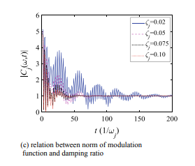
where $\bar{m}{j}$ is the $j$ th-order modal mass; $\omega{j}$ is the $j$ th-order modal frequency; $\zeta_{j}$ is the $j$ th-order modal damping ratio.
By means of the Duhamel integral, the componental formulation of the displacement of the linear system in the modal space can be derived as
$$
u_{j}(t)=\frac{1}{\bar{m}{j}} \int{0}^{t} h_{j}(t-\tau) \phi_{j}^{\mathrm{T}} \mathbf{F}(\boldsymbol{\Theta}, \tau) \mathrm{d} \tau
$$
where $u_{j}(t)$ is referred to as the $j$ th-order modal displacement.
The displacement solution of the linear system in the original state space is then given by
$$
\mathbf{X}(t)=\sum_{j=1}^{q} \frac{1}{\bar{m}{j}} \int{0}^{t} h_{j}(t-\tau) \phi_{j} \phi_{j}^{\mathrm{T}} \mathbf{F}(\boldsymbol{\Theta}, \tau) \mathrm{d} \tau
$$
Further, the mean and correlation function of the displacement can be deduced as follows:
$$
\mu_{\mathbf{X}}(t)=E[\mathbf{X}(t)]=\sum_{j=1}^{q} \frac{1}{\bar{m}{j}} \int{0}^{t} h_{j}(t-\tau) \phi_{j} \phi_{j}^{\mathrm{T}} \mu_{\mathbf{F}}(\tau) \mathrm{d} \tau
$$
统计代写|随机控制代写Stochastic Control代考|Pseudo-Excitation Method
When the linear system exhibits a high dimension, solving the power spectral density (PSD) of the system response shown in Eq. (2.3.27) involves a complicated procedure. The pseudo-excitation method (PEM) could be employed to obtain the PSD solution in an elegant manner (Lin et al. 2001). This method decomposes the solving procedure into a series of deterministic harmonic analysis through constructing a
pseudo-harmonic excitation. This treatment can enhance the efficiency of numerical schemes significantly.
Denoting the PSD of the random excitation $\mathbf{F}(\boldsymbol{\Theta}, t)$ as $\mathbf{S}{\mathbf{F}}(\omega)$, a pseudo-harmonic excitation $\mathbf{F}=\widetilde{\mathbf{F}}{\sqrt{\mathbf{s}}} \mathrm{e}^{\mathrm{i} \omega t}$ can be readily constructed, where $\widetilde{\mathbf{F}}{\sqrt{\mathbf{s}}}$ satisfies $\widetilde{\mathbf{F}}{\sqrt{\mathbf{s}}} \cdot \widetilde{\mathbf{F}}{\sqrt{\mathbf{s}}}^{*}=$ $\mathbf{S}{\mathbf{F}}(\omega)$, i denotes the imaginary unit. Replacing the excitation in Eq. (2.3.14) by the pseudo-excitation yields
$$
\overline{\mathbf{M}} \tilde{\mathbf{U}}(t)+\overline{\mathbf{C}} \tilde{\mathbf{U}}(t)+\overline{\mathbf{K}} \tilde{\mathbf{U}}(t)=\mathbf{F}^{\mathrm{T}} \tilde{\mathbf{F}}_{\sqrt{\mathbf{s}}} \mathrm{e}^{\mathrm{i} \omega t}
$$
where $\tilde{\tilde{U}}(t), \tilde{\mathbf{U}}(t), \tilde{\mathbf{U}}(t)$ are the $n$-dimensional column vectors denoting the corresponding acceleration, velocity, and displacement to the system subjected to the pseudo-excitation, respectively.
According to the classical random vibration theory, the stationary solution of Eq. (2.3.28) can be deduced as
$$
\tilde{U}{j}(\omega, t)=\frac{1}{\bar{m}{j}} H_{j}(\omega) \phi_{j}^{\mathrm{T}} \tilde{\mathbf{F}}{\sqrt{\mathbf{s}}} \mathrm{e}^{\mathrm{i} \omega t} $$ The auto-power spectral density of system response is then derived as follows: $$ \begin{aligned} S{U_{j}} \widetilde{U}{k}(\omega) &=\widetilde{U}{j}(\omega, t) \widetilde{U}{k}^{*}(\omega, t)=\frac{1}{\bar{m}{j} \bar{m}{k}} H{j}(\omega) H_{k}(\omega) \phi_{j}^{\mathrm{T}} \widetilde{\mathbf{F}}{\sqrt{\mathbf{s}}} \widetilde{\mathbf{F}}{\sqrt{\mathbf{s}}} \phi_{k} \
&=\frac{1}{\bar{m}{j} \bar{m}{k}} H_{j}(\omega) H_{k}(\omega) \phi_{j}^{\mathrm{T}} \mathbf{S}{\mathbf{F}}(\omega) \phi{k}=S_{U_{j} U_{k}}(\omega)
\end{aligned}
$$
It is shown that in the calculation of spectral density function, the factor of pseudoharmonic excitation $\mathrm{e}^{\mathrm{i} \omega t}$ is always paired with its complex conjugate $\mathrm{e}^{-\mathrm{i} \omega t}$ which are eventually counteracted by multiplication, revealing the time-independent behaviors of auto- and cross-power spectral densities of stationary processes.
Further, one can attain the mean-square solution of system responses:
$$
E\left[\mathbf{U}(t) \mathbf{U}^{\mathrm{T}}(t)\right]=\frac{1}{2 \pi} \int_{-\infty}^{\infty} \mathbf{S}{\mathbf{U}}(\omega) \mathrm{d} \omega $$ Projecting the generalized coordinate space onto the original coordinate space, then $$ E\left[\mathbf{X}(t) \mathbf{X}^{\mathrm{T}}(t)\right]=\boldsymbol{\Phi} E\left[\mathbf{U}(t) \mathbf{U}^{\mathrm{T}}(t)\right] \boldsymbol{\Phi}^{\mathrm{T}}=\frac{1}{2 \pi} \int{-\infty}^{\infty} \boldsymbol{\Phi} \mathbf{S}_{\mathbf{U}}(\omega) \boldsymbol{\Phi}^{\mathrm{T}} \mathrm{d} \omega
$$
统计代写|随机控制代写Stochastic Control代考|Nonlinear Random Vibration
Without loss of generality, a nonlinear stochastic dynamical system is investigated, of which the equation of motion is given by
$$
\mathbf{M} \ddot{\mathbf{X}}(t)+\mathbf{f}(\mathbf{X}(t), \dot{\mathbf{X}}(t))=\mathbf{F}(\boldsymbol{\Theta}, t)
$$
where $\mathbf{f}(\cdot)$ is the $n$-dimensional column vector denoting nonlinear internal force.
The nonlinear internal force is assumed to be denoted by a polynomial function of velocity and displacement. In fact, this is a weak hypothesis, and a large family of dynamical systems can be represented by the formulation, such as the Duffing oscillator with nonlinear stiffness force and the van der Pol oscillator with coupling nonlinearities between stiffness and damping forces. The componental form of the equation is then written as
$$
\sum_{i=1}^{n} m_{j i} \ddot{x}{i}(t)+\sum{i=1}^{n} \sum_{k=0}^{q} \alpha_{j i, k} \dot{x}{i}^{q-k}(t) x{i}^{k}(t)=F_{j}(\boldsymbol{\Theta}, t)
$$
where $j=1,2, \ldots, n, m_{j i}$ denotes the element of mass matrix; $\ddot{x}{i}(t), \dot{x}{i}(t), x_{i}(t)$ denote the acceleration, velocity, and displacement pertaining to the $i$ th component, respectively; $q$ denotes the highest order of the polynomial function of the internal
force; $\alpha_{j i, k}$ denotes the coefficient of the polynomial function. As the highest order $q$ is set as 1, Eq. (2.3.35) is reduced to a linear formulation:
$$
\sum_{i=1}^{n} m_{j i} \ddot{x}{i}(t)+\sum{i=1}^{n} \alpha_{j i, 0} \dot{x}{i}(t)+\sum{i=1}^{n} \alpha_{j i, 1} x_{i}(t)=F_{j}(\Theta, t)
$$
where $\alpha_{j i, 0}, \alpha_{j i, 1}$ denote the coefficients relevant to damping force and the restoring force, respectively.
随机控制代写
统计代写|随机控制代写Stochastic Control代考|Modal Superposition Method
在实际应用中,求单位冲激响应函数解析解的复杂度H(吨)远远超过频率响应传递函数H(ω)对于多自由度系统。此外,均方响应的求解过程通常涉及对单位脉冲响应函数和频率响应传递函数的高维积分。在大多数情况下,计算成本是不可接受的。实际上,对于线性随机动力系统,一种减少工作量的方式是指所谓的模态叠加法。基本思想是原来的多自由度
将随机系统解耦为一系列单自由度随机系统,从而显着降低计算成本。
根据模态叠加法的原理,随机动力系统的运动方程如式(1)所示。(2.3.1) 可以改写为
米¯在¨(吨)+C¯在˙(吨)+ķ¯在(吨)=披吨F(θ,吨)
在哪里米¯=披吨米披,C¯=披吨C披,ķ¯=披吨ķ披是n×n分别为模态质量、模态阻尼和模态刚度矩阵;在=披吨X是个n-表示模态位移的维列向量;披=[φ1,φ2,…,φq]=[φ一世j]n×q (q≤n)是模态矩阵。
假设阻尼矩阵C是比例阻尼矩阵,方程式。(2.3.14)可以分解为q相互独立的单自由度系统,其中的运动方程j三阶模式如下图所示:
在¨一世(吨)+2G一世ω一世在˙一世(吨)+ωj2在一世(吨)=1米¯jφj吨F(θ,吨)=1米¯j∑ķ=1nφ一世ķFķ(θ,吨),j=1,2,…,q
在哪里米¯j是个j三阶模态质量;ωj是个j三阶模态频率;Gj是个j三阶模态阻尼比。
通过 Duhamel 积分,线性系统在模态空间中的位移分量公式可以推导出为
在j(吨)=1米¯j∫0吨Hj(吨−τ)φj吨F(θ,τ)dτ
在哪里在j(吨)被称为j三阶模态位移。
线性系统在原始状态空间中的位移解由下式给出
X(吨)=∑j=1q1米¯j∫0吨Hj(吨−τ)φjφj吨F(θ,τ)dτ
进一步,位移的均值和相关函数可以推导出如下:
μX(吨)=和[X(吨)]=∑j=1q1米¯j∫0吨Hj(吨−τ)φjφj吨μF(τ)dτ
统计代写|随机控制代写Stochastic Control代考|Pseudo-Excitation Method
当线性系统呈现高维时,求解方程中所示系统响应的功率谱密度(PSD)。(2.3.27) 涉及一个复杂的程序。可以采用伪激发方法 (PEM) 以优雅的方式获得 PSD 解决方案 (Lin et al. 2001)。该方法将求解过程分解为一系列确定性谐波分析,通过构造一个
伪谐波激励。这种处理可以显着提高数值方案的效率。
表示随机激励的 PSDF(θ,吨)作为小号F(ω), 一个伪谐波激励F=F~s和一世ω吨可以很容易地构建,其中F~s满足F~s⋅F~s∗= 小号F(ω), i 表示虚数单位。替换方程式中的激励。(2.3.14) 由伪激发产生
米¯在~(吨)+C¯在~(吨)+ķ¯在~(吨)=F吨F~s和一世ω吨
在哪里在~~(吨),在~(吨),在~(吨)是n维列向量分别表示受到伪激励的系统的相应加速度、速度和位移。
根据经典随机振动理论,方程的平稳解。(2.3.28) 可以推导出为
在~j(ω,吨)=1米¯jHj(ω)φj吨F~s和一世ω吨然后导出系统响应的自功率谱密度如下:
小号在j在~ķ(ω)=在~j(ω,吨)在~ķ∗(ω,吨)=1米¯j米¯ķHj(ω)Hķ(ω)φj吨F~sF~sφķ =1米¯j米¯ķHj(ω)Hķ(ω)φj吨小号F(ω)φķ=小号在j在ķ(ω)
结果表明,在谱密度函数的计算中,赝谐波激励因子和一世ω吨总是与其复共轭配对和−一世ω吨最终被乘法抵消,揭示了平稳过程的自功率谱密度和互功率谱密度与时间无关的行为。
此外,可以得到系统响应的均方解:
和[在(吨)在吨(吨)]=12圆周率∫−∞∞小号在(ω)dω将广义坐标空间投影到原始坐标空间上,然后
和[X(吨)X吨(吨)]=披和[在(吨)在吨(吨)]披吨=12圆周率∫−∞∞披小号在(ω)披吨dω
统计代写|随机控制代写Stochastic Control代考|Nonlinear Random Vibration
不失一般性,研究了一个非线性随机动力系统,其运动方程为
米X¨(吨)+F(X(吨),X˙(吨))=F(θ,吨)
在哪里F(⋅)是个n维列向量表示非线性内力。
假设非线性内力由速度和位移的多项式函数表示。事实上,这是一个弱假设,并且可以用该公式表示一大类动力系统,例如具有非线性刚度力的 Duffing 振子和具有刚度和阻尼力之间耦合非线性的 van der Pol 振子。然后方程的分量形式写为
∑一世=1n米j一世X¨一世(吨)+∑一世=1n∑ķ=0q一种j一世,ķX˙一世q−ķ(吨)X一世ķ(吨)=Fj(θ,吨)
在哪里j=1,2,…,n,米j一世表示质量矩阵的元素;X¨一世(吨),X˙一世(吨),X一世(吨)表示加速度、速度和位移与一世分量,分别;q表示内部多项式函数的最高阶
力量;一种j一世,ķ表示多项式函数的系数。作为最高阶q设置为 1,方程式。(2.3.35) 简化为线性公式:
∑一世=1n米j一世X¨一世(吨)+∑一世=1n一种j一世,0X˙一世(吨)+∑一世=1n一种j一世,1X一世(吨)=Fj(θ,吨)
在哪里一种j一世,0,一种j一世,1分别表示与阻尼力和恢复力相关的系数。

统计代写请认准statistics-lab™. statistics-lab™为您的留学生涯保驾护航。
金融工程代写
金融工程是使用数学技术来解决金融问题。金融工程使用计算机科学、统计学、经济学和应用数学领域的工具和知识来解决当前的金融问题,以及设计新的和创新的金融产品。
非参数统计代写
非参数统计指的是一种统计方法,其中不假设数据来自于由少数参数决定的规定模型;这种模型的例子包括正态分布模型和线性回归模型。
广义线性模型代考
广义线性模型(GLM)归属统计学领域,是一种应用灵活的线性回归模型。该模型允许因变量的偏差分布有除了正态分布之外的其它分布。
术语 广义线性模型(GLM)通常是指给定连续和/或分类预测因素的连续响应变量的常规线性回归模型。它包括多元线性回归,以及方差分析和方差分析(仅含固定效应)。
有限元方法代写
有限元方法(FEM)是一种流行的方法,用于数值解决工程和数学建模中出现的微分方程。典型的问题领域包括结构分析、传热、流体流动、质量运输和电磁势等传统领域。
有限元是一种通用的数值方法,用于解决两个或三个空间变量的偏微分方程(即一些边界值问题)。为了解决一个问题,有限元将一个大系统细分为更小、更简单的部分,称为有限元。这是通过在空间维度上的特定空间离散化来实现的,它是通过构建对象的网格来实现的:用于求解的数值域,它有有限数量的点。边界值问题的有限元方法表述最终导致一个代数方程组。该方法在域上对未知函数进行逼近。[1] 然后将模拟这些有限元的简单方程组合成一个更大的方程系统,以模拟整个问题。然后,有限元通过变化微积分使相关的误差函数最小化来逼近一个解决方案。
tatistics-lab作为专业的留学生服务机构,多年来已为美国、英国、加拿大、澳洲等留学热门地的学生提供专业的学术服务,包括但不限于Essay代写,Assignment代写,Dissertation代写,Report代写,小组作业代写,Proposal代写,Paper代写,Presentation代写,计算机作业代写,论文修改和润色,网课代做,exam代考等等。写作范围涵盖高中,本科,研究生等海外留学全阶段,辐射金融,经济学,会计学,审计学,管理学等全球99%专业科目。写作团队既有专业英语母语作者,也有海外名校硕博留学生,每位写作老师都拥有过硬的语言能力,专业的学科背景和学术写作经验。我们承诺100%原创,100%专业,100%准时,100%满意。
随机分析代写
随机微积分是数学的一个分支,对随机过程进行操作。它允许为随机过程的积分定义一个关于随机过程的一致的积分理论。这个领域是由日本数学家伊藤清在第二次世界大战期间创建并开始的。
时间序列分析代写
随机过程,是依赖于参数的一组随机变量的全体,参数通常是时间。 随机变量是随机现象的数量表现,其时间序列是一组按照时间发生先后顺序进行排列的数据点序列。通常一组时间序列的时间间隔为一恒定值(如1秒,5分钟,12小时,7天,1年),因此时间序列可以作为离散时间数据进行分析处理。研究时间序列数据的意义在于现实中,往往需要研究某个事物其随时间发展变化的规律。这就需要通过研究该事物过去发展的历史记录,以得到其自身发展的规律。
回归分析代写
多元回归分析渐进(Multiple Regression Analysis Asymptotics)属于计量经济学领域,主要是一种数学上的统计分析方法,可以分析复杂情况下各影响因素的数学关系,在自然科学、社会和经济学等多个领域内应用广泛。
MATLAB代写
MATLAB 是一种用于技术计算的高性能语言。它将计算、可视化和编程集成在一个易于使用的环境中,其中问题和解决方案以熟悉的数学符号表示。典型用途包括:数学和计算算法开发建模、仿真和原型制作数据分析、探索和可视化科学和工程图形应用程序开发,包括图形用户界面构建MATLAB 是一个交互式系统,其基本数据元素是一个不需要维度的数组。这使您可以解决许多技术计算问题,尤其是那些具有矩阵和向量公式的问题,而只需用 C 或 Fortran 等标量非交互式语言编写程序所需的时间的一小部分。MATLAB 名称代表矩阵实验室。MATLAB 最初的编写目的是提供对由 LINPACK 和 EISPACK 项目开发的矩阵软件的轻松访问,这两个项目共同代表了矩阵计算软件的最新技术。MATLAB 经过多年的发展,得到了许多用户的投入。在大学环境中,它是数学、工程和科学入门和高级课程的标准教学工具。在工业领域,MATLAB 是高效研究、开发和分析的首选工具。MATLAB 具有一系列称为工具箱的特定于应用程序的解决方案。对于大多数 MATLAB 用户来说非常重要,工具箱允许您学习和应用专业技术。工具箱是 MATLAB 函数(M 文件)的综合集合,可扩展 MATLAB 环境以解决特定类别的问题。可用工具箱的领域包括信号处理、控制系统、神经网络、模糊逻辑、小波、仿真等。