如果你也在 怎样代写机器学习machine learning这个学科遇到相关的难题,请随时右上角联系我们的24/7代写客服。
机器学习(ML)是人工智能(AI)的一种类型,它允许软件应用程序在预测结果时变得更加准确,而无需明确编程。机器学习算法使用历史数据作为输入来预测新的输出值。
statistics-lab™ 为您的留学生涯保驾护航 在代写机器学习machine learning方面已经树立了自己的口碑, 保证靠谱, 高质且原创的统计Statistics代写服务。我们的专家在代写机器学习machine learning代写方面经验极为丰富,各种代写机器学习machine learning相关的作业也就用不着说。
我们提供的机器学习machine learning及其相关学科的代写,服务范围广, 其中包括但不限于:
- Statistical Inference 统计推断
- Statistical Computing 统计计算
- Advanced Probability Theory 高等概率论
- Advanced Mathematical Statistics 高等数理统计学
- (Generalized) Linear Models 广义线性模型
- Statistical Machine Learning 统计机器学习
- Longitudinal Data Analysis 纵向数据分析
- Foundations of Data Science 数据科学基础
计算机代写|机器学习代写machine learning代考|Set Theory
A set describes an ensemble of elements, also referred to as events. An elementary event $x$ refers to a single event among a sampling space (or universe) denoted by the calligraphic letter $\mathcal{S}$. By definition, a sampling space contains all the possible events, $E \subseteq \mathcal{S}$. The special case where an event is equal to the sampling space, $E=\mathcal{S}$, is called a certain event. The opposite, $E=\emptyset$, where an event is an empty set, is called a null event. $E$ refers to the complement of a set, that is, all elements belonging to $\mathcal{S}$ and not to $E$. Figure $3.3$ illustrates these concepts using a Venn diagram.
Let us consider the example, ${ }^{5}$ of the state of a structure following an earthquake, which is described by a sampling space,
$$
\begin{aligned}
\mathcal{S} &={\text { no damage, light damage, important damage, collapse }} \
&={N, L, I, C} .
\end{aligned}
$$
In that context, an event $E_{1}={\mathbf{N}, \mathrm{L}}$ could contain the no damage and light damage events, and another event $E_{2}={C}$ could contain only the collapsed state. The complements of these events are, respectively, $\overline{E_{1}}={\mathrm{I}, \mathrm{C}}$ and $\overline{E_{2}}={\mathrm{N}, \mathrm{L}, \mathrm{I}}$.
The two main operations for events, union and intersection, are illustrated in figure 3.4. A union is analogous to the “or” operator, where $E_{1} \cup E_{2}$ holds if the event belongs to either $E_{1}, E_{2}$, or both. The intersection is analogous to the “and” operator, where $E_{1} \backslash E_{2} \equiv E_{1} E_{2}$ holds if the event belongs to both $E_{1}$ and $E_{2}$. As a convention, intersection has priority over union. Moreover, both operations are commutative, associative, and distributive.
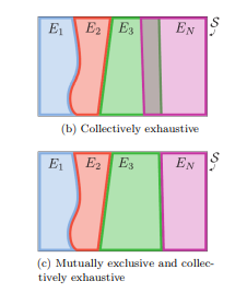
Given a set of $n$ events $\left{E_{1}, E_{2}, \cdots, E_{n}\right} \in \mathcal{S}, E_{1}, E_{2}, \cdots, E_{n}$,the events are mutually exclusive if $E_{i} E_{j}=\emptyset, \forall i \neq j$, that is, if the intersection for any pair of events is an empty set. Events $E_{1}, E_{2}, \cdots, E_{n}$ are collectively exhaustive if $\cup_{i=1}^{n} E_{i}=\mathcal{S}$, that is, the union of all events is the sampling space. Events $E_{1}, E_{2}, \cdots, E_{n}$ are mutually exclusive and collectively exhaustive if they satisfy both properties simultaneously. Figure $3.5$ presents examples of mutually exclusive (3.5a), collectively exhaustive (3.5b), and mutually exclusive and collectively exhaustive $(3.5 \mathrm{c}-\mathrm{d})$ events. Note that the difference between (b) and (c) is the absence of overlap in the latter.
计算机代写|机器学习代写machine learning代考|Probability of Events
$\operatorname{Pr}\left(E_{i}\right)$ denotes the probability of the event $E_{i}$. There are two main interpretations for a probability: the Frequentist and the Bayesian. Frequentists interpret a probability as the number of occurrences of $E_{i}$ relative to the number of samples $s$, as $s$ goes to $\infty$,
$$
\operatorname{Pr}\left(E_{i}\right)=\lim {s \rightarrow \infty} \frac{#\left{E{i}\right}}{s} .
$$
For Bayesians, a probability measures how likely is $E_{i}$ in comparison with other events in $\mathcal{S}$. This interpretation assumes that the nature of uncertainty is epistemic, that is, it describes our knowledge of a phenomenon. For instance, the probability depends on the available knowledge and can change when new information is obtained. Throughout this book we are adopting this Bayesian interpretation.
By definition, the probability of an event is a number between zero and one, $0 \leq \operatorname{Pr}\left(E_{i}\right) \leq 1$. At the ends of this spectrum, the probability of any event in $\mathcal{S}$ is one, $\operatorname{Pr}(\mathcal{S})=1$, and the probability of an empty set is zero, $\operatorname{Pr}(\emptyset)=0$. If two events $E_{1}$ and $E_{2}$ are mutually exclusive, then the probability of the events’ union is the sum of each event’s probability. Because the union of an event and its complement are the sampling space, $E \cup E=\mathcal{S}$ (see figure $3.5 \mathrm{~d}$ ), and because $\operatorname{Pr}(\mathcal{S})=1$, then the probability of the complement is $\operatorname{Pr}(E)=1-\operatorname{Pr}(E)$.
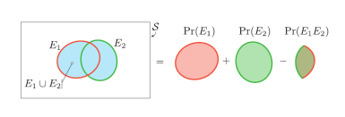
When events are not mutually exclusive, the general addition rule for the probability of the union of two events is
$$
\operatorname{Pr}\left(E_{1} \cup E_{2}\right)=\operatorname{Pr}\left(E_{1}\right)+\operatorname{Pr}\left(E_{2}\right)-\operatorname{Pr}\left(E_{1} E_{2}\right) .
$$
This general addition rule is illustrated in figure 3.6, where if we simply add the probability of each event without accounting for the subtraction of $\operatorname{Pr}\left(E_{1} E_{2}\right)$, the probability of the intersection of both events will be counted twice.
计算机代写|机器学习代写machine learning代考|The probability of a single e
The probability of a single event is referred to as a maryinal probability. A joint probability designates the probability of the intersection of events. The terms in equation $3.1$ can be rearranged to explicitly show that the joint probability of two events $\left{E_{1}, E_{2}\right}$ is the product of a conditional probability and its associated marginal,
$$
\begin{aligned}
\operatorname{Pr}\left(E_{1} E_{2}\right) &=\operatorname{Pr}\left(E_{1} \mid E_{2}\right) \cdot \operatorname{Pr}\left(E_{2}\right) \
&=\operatorname{Pr}\left(E_{2} \mid E_{1}\right) \cdot \operatorname{Pr}\left(E_{1}\right) .
\end{aligned}
$$
In cases where $E_{1}$ and $E_{2}$ are statistically independent, $E_{1} \perp E_{2}$,
Note: Statis conditional probabilities are equal to the marginal, tween a pair
$$
E_{1} \perp E_{2} \begin{cases}\operatorname{Pr}\left(E_{1} \mid E_{2}\right)=\operatorname{Pr}\left(E_{1}\right) & \text { that learning } \ \operatorname{Pr}\left(E_{2} \mid E_{1}\right)=\operatorname{Pr}\left(E_{2}\right) & \text { other. }\end{cases}
$$
In the special case of statistically independent events, the joint probability reduces to the product of the marginals,
$$
\operatorname{Pr}\left(E_{1} E_{2}\right)=\operatorname{Pr}\left(E_{1}\right) \cdot \operatorname{Pr}\left(E_{2}\right)
$$
The joint probability for $n$ events can be broken down into $n-1$ conditionals and one marginal probability using the chain rule,
$$
\begin{aligned}
\operatorname{Pr}\left(E_{1} E_{2} \cdots E_{n}\right) &=\operatorname{Pr}\left(E_{1} \mid E_{2} \cdots E_{n}\right) \operatorname{Pr}\left(E_{2} \cdots E_{n}\right) \
&=\operatorname{Pr}\left(E_{1} \mid E_{2} \cdots E_{n}\right) \operatorname{Pr}\left(E_{2} \mid E_{3} \cdots E_{n}\right) \operatorname{Pr}\left(E_{3} \cdots E_{n}\right) \
&=\operatorname{Pr}\left(E_{1} \mid E_{2} \cdots E_{n}\right) \operatorname{Pr}\left(E_{2} \mid E_{3} \cdots E_{n}\right) \cdots \operatorname{Pr}\left(E_{n-1} \mid E_{n}\right) \operatorname{Pr}\left(E_{n}\right)
\end{aligned}
$$
Let us define $\left{E_{1}, E_{2}, E_{3}, \cdots, E_{n}\right} \in \mathcal{S}$, a set of mutually exclusive and collectively exhaustive events, that is, $E_{i} E_{j}=\emptyset, \forall i \neq$ $j, \cup_{i=1}^{n} E_{i}=\mathcal{S}$ – and an event $A$ belonging to the same sampling
space, that is, $A \in \mathcal{S}$. This context is illustrated using a Venn diagram in figure 3.7. The probability of the event $A$ can be obtained by summing the joint probability of $A$ and each event $E_{i}$,
$$
\operatorname{Pr}(A)=\sum_{i=1}^{n} \underbrace{\operatorname{Pr}\left(A \mid E_{i}\right) \cdot \operatorname{Pr}\left(E_{i}\right)}{\operatorname{Pr}\left(A E{i}\right)} .
$$
机器学习代考
计算机代写|机器学习代写machine learning代考|Set Theory
集合描述元素的集合,也称为事件。一个初级事件X指在一个由书法字母表示的采样空间(或宇宙)中的单个事件小号. 根据定义,一个采样空间包含所有可能的事件,和⊆小号. 事件等于采样空间的特殊情况,和=小号,称为某个事件。反之,和=∅,其中一个事件是一个空集,称为空事件。和指一个集合的补集,即所有属于的元素小号而不是和. 数字3.3使用维恩图说明这些概念。
让我们考虑这个例子,5地震后结构的状态,由采样空间描述,
小号= 无损坏、轻微损坏、重要损坏、倒塌 =ñ,大号,我,C.
在这种情况下,一个事件和1=ñ,大号可以包含无伤害和轻伤害事件,以及另一个事件和2=C只能包含折叠状态。这些事件的补充分别是,和1¯=我,C和和2¯=ñ,大号,我.
事件的两个主要操作,联合和交集,如图 3.4 所示。联合类似于“或”运算符,其中和1∪和2如果事件属于任何一个,则成立和1,和2, 或两者。交集类似于“与”运算符,其中和1∖和2≡和1和2如果事件属于两者,则成立和1和和2. 按照惯例,交集优先于并集。此外,这两种操作都是可交换的、关联的和分配的。
给定一组n事件\left{E_{1}, E_{2}, \cdots, E_{n}\right} \in \mathcal{S}, E_{1}, E_{2}, \cdots, E_{n}\left{E_{1}, E_{2}, \cdots, E_{n}\right} \in \mathcal{S}, E_{1}, E_{2}, \cdots, E_{n}, 事件是互斥的,如果和一世和j=∅,∀一世≠j,也就是说,如果任何一对事件的交集是一个空集。活动和1,和2,⋯,和n是集体详尽的,如果∪一世=1n和一世=小号,即所有事件的并集就是采样空间。活动和1,和2,⋯,和n如果它们同时满足这两个属性,则它们是相互排斥的并且是集体穷举的。数字3.5提供互斥 (3.5a)、集体穷举 (3.5b) 和互斥和集体穷举的例子(3.5C−d)事件。请注意,(b)和(c)之间的区别在于后者没有重叠。
计算机代写|机器学习代写machine learning代考|Probability of Events
公关(和一世)表示事件的概率和一世. 概率有两种主要解释:频率派和贝叶斯派。频率论者将概率解释为发生的次数和一世相对于样本数量s, 作为s去∞,
\operatorname{Pr}\left(E_{i}\right)=\lim {s \rightarrow \infty} \frac{#\left{E{i}\right}}{s} 。\operatorname{Pr}\left(E_{i}\right)=\lim {s \rightarrow \infty} \frac{#\left{E{i}\right}}{s} 。
对于贝叶斯,概率衡量的是可能性有多大和一世与其他事件相比小号. 这种解释假设不确定性的本质是认知的,也就是说,它描述了我们对现象的认识。例如,概率取决于可用的知识,并且在获得新信息时会发生变化。在整本书中,我们都采用了这种贝叶斯解释。
根据定义,事件的概率是一个介于 0 和 1 之间的数字,0≤公关(和一世)≤1. 在这个频谱的末端,任何事件发生的概率小号是一个,公关(小号)=1,空集的概率为零,公关(∅)=0. 如果两个事件和1和和2是互斥的,则事件联合的概率是每个事件的概率之和。因为一个事件的并集和它的补集是采样空间,和∪和=小号(见图3.5 d),并且因为公关(小号)=1,则补码的概率为公关(和)=1−公关(和).
当事件不互斥时,两个事件并集概率的一般加法规则是
公关(和1∪和2)=公关(和1)+公关(和2)−公关(和1和2).
这个一般的加法规则如图 3.6 所示,如果我们只是简单地将每个事件的概率相加,而不考虑减去公关(和1和2),两个事件相交的概率将被计算两次。
计算机代写|机器学习代写machine learning代考|The probability of a single e
单个事件的概率称为马里纳尔概率。联合概率表示事件相交的概率。方程中的项3.1可以重新排列以明确显示两个事件的联合概率\left{E_{1}, E_{2}\right}\left{E_{1}, E_{2}\right}是条件概率及其相关边际的乘积,
公关(和1和2)=公关(和1∣和2)⋅公关(和2) =公关(和2∣和1)⋅公关(和1).
在这种情况下和1和和2是统计独立的,和1⊥和2,
注:Statis 条件概率等于边际,补间一对
和1⊥和2{公关(和1∣和2)=公关(和1) 那个学习 公关(和2∣和1)=公关(和2) 其他。
在统计独立事件的特殊情况下,联合概率减少到边际的乘积,
公关(和1和2)=公关(和1)⋅公关(和2)
联合概率为n事件可以分解为n−1使用链式法则的条件和一个边际概率,
公关(和1和2⋯和n)=公关(和1∣和2⋯和n)公关(和2⋯和n) =公关(和1∣和2⋯和n)公关(和2∣和3⋯和n)公关(和3⋯和n) =公关(和1∣和2⋯和n)公关(和2∣和3⋯和n)⋯公关(和n−1∣和n)公关(和n)
让我们定义\left{E_{1}, E_{2}, E_{3}, \cdots, E_{n}\right} \in \mathcal{S}\left{E_{1}, E_{2}, E_{3}, \cdots, E_{n}\right} \in \mathcal{S},一组相互排斥且共同穷举的事件,即,和一世和j=∅,∀一世≠ j,∪一世=1n和一世=小号– 和一个事件一个属于同一样本
空间,也就是说,一个∈小号. 使用图 3.7 中的维恩图说明了这种情况。事件的概率一个可以通过对联合概率求和得到一个和每一个事件和一世,
公关(一个)=∑一世=1n公关(一个∣和一世)⋅公关(和一世)⏟公关(一个和一世).

统计代写请认准statistics-lab™. statistics-lab™为您的留学生涯保驾护航。
金融工程代写
金融工程是使用数学技术来解决金融问题。金融工程使用计算机科学、统计学、经济学和应用数学领域的工具和知识来解决当前的金融问题,以及设计新的和创新的金融产品。
非参数统计代写
非参数统计指的是一种统计方法,其中不假设数据来自于由少数参数决定的规定模型;这种模型的例子包括正态分布模型和线性回归模型。
广义线性模型代考
广义线性模型(GLM)归属统计学领域,是一种应用灵活的线性回归模型。该模型允许因变量的偏差分布有除了正态分布之外的其它分布。
术语 广义线性模型(GLM)通常是指给定连续和/或分类预测因素的连续响应变量的常规线性回归模型。它包括多元线性回归,以及方差分析和方差分析(仅含固定效应)。
有限元方法代写
有限元方法(FEM)是一种流行的方法,用于数值解决工程和数学建模中出现的微分方程。典型的问题领域包括结构分析、传热、流体流动、质量运输和电磁势等传统领域。
有限元是一种通用的数值方法,用于解决两个或三个空间变量的偏微分方程(即一些边界值问题)。为了解决一个问题,有限元将一个大系统细分为更小、更简单的部分,称为有限元。这是通过在空间维度上的特定空间离散化来实现的,它是通过构建对象的网格来实现的:用于求解的数值域,它有有限数量的点。边界值问题的有限元方法表述最终导致一个代数方程组。该方法在域上对未知函数进行逼近。[1] 然后将模拟这些有限元的简单方程组合成一个更大的方程系统,以模拟整个问题。然后,有限元通过变化微积分使相关的误差函数最小化来逼近一个解决方案。
tatistics-lab作为专业的留学生服务机构,多年来已为美国、英国、加拿大、澳洲等留学热门地的学生提供专业的学术服务,包括但不限于Essay代写,Assignment代写,Dissertation代写,Report代写,小组作业代写,Proposal代写,Paper代写,Presentation代写,计算机作业代写,论文修改和润色,网课代做,exam代考等等。写作范围涵盖高中,本科,研究生等海外留学全阶段,辐射金融,经济学,会计学,审计学,管理学等全球99%专业科目。写作团队既有专业英语母语作者,也有海外名校硕博留学生,每位写作老师都拥有过硬的语言能力,专业的学科背景和学术写作经验。我们承诺100%原创,100%专业,100%准时,100%满意。
随机分析代写
随机微积分是数学的一个分支,对随机过程进行操作。它允许为随机过程的积分定义一个关于随机过程的一致的积分理论。这个领域是由日本数学家伊藤清在第二次世界大战期间创建并开始的。
时间序列分析代写
随机过程,是依赖于参数的一组随机变量的全体,参数通常是时间。 随机变量是随机现象的数量表现,其时间序列是一组按照时间发生先后顺序进行排列的数据点序列。通常一组时间序列的时间间隔为一恒定值(如1秒,5分钟,12小时,7天,1年),因此时间序列可以作为离散时间数据进行分析处理。研究时间序列数据的意义在于现实中,往往需要研究某个事物其随时间发展变化的规律。这就需要通过研究该事物过去发展的历史记录,以得到其自身发展的规律。
回归分析代写
多元回归分析渐进(Multiple Regression Analysis Asymptotics)属于计量经济学领域,主要是一种数学上的统计分析方法,可以分析复杂情况下各影响因素的数学关系,在自然科学、社会和经济学等多个领域内应用广泛。
MATLAB代写
MATLAB 是一种用于技术计算的高性能语言。它将计算、可视化和编程集成在一个易于使用的环境中,其中问题和解决方案以熟悉的数学符号表示。典型用途包括:数学和计算算法开发建模、仿真和原型制作数据分析、探索和可视化科学和工程图形应用程序开发,包括图形用户界面构建MATLAB 是一个交互式系统,其基本数据元素是一个不需要维度的数组。这使您可以解决许多技术计算问题,尤其是那些具有矩阵和向量公式的问题,而只需用 C 或 Fortran 等标量非交互式语言编写程序所需的时间的一小部分。MATLAB 名称代表矩阵实验室。MATLAB 最初的编写目的是提供对由 LINPACK 和 EISPACK 项目开发的矩阵软件的轻松访问,这两个项目共同代表了矩阵计算软件的最新技术。MATLAB 经过多年的发展,得到了许多用户的投入。在大学环境中,它是数学、工程和科学入门和高级课程的标准教学工具。在工业领域,MATLAB 是高效研究、开发和分析的首选工具。MATLAB 具有一系列称为工具箱的特定于应用程序的解决方案。对于大多数 MATLAB 用户来说非常重要,工具箱允许您学习和应用专业技术。工具箱是 MATLAB 函数(M 文件)的综合集合,可扩展 MATLAB 环境以解决特定类别的问题。可用工具箱的领域包括信号处理、控制系统、神经网络、模糊逻辑、小波、仿真等。