如果你也在 怎样代写量化风险管理Quantitative Risk Management这个学科遇到相关的难题,请随时右上角联系我们的24/7代写客服。
项目管理中的定量风险管理是将风险对项目的影响转换为数字的过程。这种数字信息经常被用来确定项目的成本和时间应急措施。
statistics-lab™ 为您的留学生涯保驾护航 在代写量化风险管理Quantitative Risk Management方面已经树立了自己的口碑, 保证靠谱, 高质且原创的统计Statistics代写服务。我们的专家在代写量化风险管理Quantitative Risk Management代写方面经验极为丰富,各种代写量化风险管理Quantitative Risk Management相关的作业也就用不着说。
我们提供的量化风险管理Quantitative Risk Management及其相关学科的代写,服务范围广, 其中包括但不限于:
- Statistical Inference 统计推断
- Statistical Computing 统计计算
- Advanced Probability Theory 高等概率论
- Advanced Mathematical Statistics 高等数理统计学
- (Generalized) Linear Models 广义线性模型
- Statistical Machine Learning 统计机器学习
- Longitudinal Data Analysis 纵向数据分析
- Foundations of Data Science 数据科学基础
金融代写|量化风险管理代写Quantitative Risk Management代考|Semi-Interquartile Deviation
The semi-interquartile deviation or range ${ }^{2}$ corresponds to one-half of the interquartile range, i.e., the difference between the third quartile $(\mathrm{Q} 3)$ and the first $(\mathrm{Q} 1)$ and the coefficient of quartile variation is the interquartile range divided by the second quartile. Formally, the semi-interquartile range, measuring the dispersion, is expressed as follows:
$$
S I=\frac{(Q 3-Q 1)}{2}
$$
while the coefficient of quartile variation is expressed as follows:
$$
S I=\frac{(Q 3-Q 1)}{Q 2}
$$
In a symmetric distribution, contrary to a skewed distribution, an interval stretching from one semi-interquartile range below the median to one semi-interquartile above the median will contain half of the values.
It is interesting to mention that semi-interquartile range is barely affected by extreme values, as a consequence it is a good dispersion measure for skewed distributions. However, it is more subject to sampling fluctuation in the Gaussian case than is the standard deviation and therefore not often used for data that are approximately normally distributed.
However, this class of risk measure exhibits the major drawbacks of assuming distribution with specific characteristics such as symmetry and of not take into account losses occurring with small probabilities.
金融代写|量化风险管理代写Quantitative Risk Management代考|Mean Absolute Difference
Assuming the probability space defined in introduction, let $X$ and $Y$ be two iid random variables following the same distribution. The mean absolute difference (MAD) is given by the average of the differences of all possible pairs of variatevalues, taken regardless of their sign. It is formally defined as follows:
$$
\mathrm{MAD}:=E[|X-Y|] .
$$
Let $x_{1}, \ldots, x_{n}$ and $y_{1}, \ldots, y_{n}$ be two sets of respective realisations of random variables $X$ and $Y$. For a random sample of size $n$ of a population uniformly distributed, by the law of total expectation ${ }^{3}$ the mean absolute difference of the sample $y_{i}, i=1$ to $n$ corresponds to the arithmetic mean of the absolute value of all possible differences,
$$
\mathrm{MAD}=E[|X-Y|]=E_{X}\left[E_{X|Y|}[|X-Y|]\right]=\frac{1}{n^{2}} \sum_{i=1}^{n} \sum_{j=1}^{n}\left|y_{i}-y_{j}\right| .
$$
If $Y$ follows a discrete probability function $f(y)$, where $y_{i}, i=1$ to $n$ are the values with non-zero probabilities:
$$
\mathrm{MAD}=\sum_{i=1}^{n} \sum_{j=1}^{n} f\left(y_{i}\right) f\left(y_{j}\right)\left|y_{i}-y_{j}\right|
$$
In the continuous case, let $f(x)$ be the probability density function, then,
$$
\mathrm{MAD}=\int_{-\infty}^{\infty} \int_{-\infty}^{\infty} f(x) f(y)|x-y| d x d y
$$
Let $F(x)$, absolutely continuous, be the cumulative distribution function associated with $f(x)$ with quantile function $F^{-1}(x)$, then, since $f(x)=d F(x) / d x$ and $F^{-1}(x)=x$, it follows that:
$$
\mathrm{MAD}=\int_{0}^{1} \int_{0}^{1}\left|F_{1}^{-1}-F_{2}^{-1}\right| d F_{1} d F_{2} .
$$
金融代写|量化风险管理代写Quantitative Risk Management代考|Modern Portfolio Theory
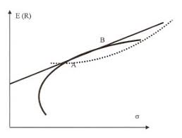
Modern portfolio theory (Markowitz 1952) is a mathematical framework for constituting a portfolio of assets such that the expected return is maximised for a given level of risk, here the variance. The difference with what we discussed before is that both risk and return of an asset should not be assessed on their own, but by how it contributes to a portfolio’s overall risk and return.
Modern portfolio theory assumes that investors are risk averse that for the same expected return given by two portfolios, investors will prefer the less risky one. As a consequence, an investor may only accept on increased exposure if this one is compensated by higher expected returns. Conversely, an investor who is willing higher expected returns must face larger exposures. The exact trade-off will be the same for all investors, but different investors will evaluate the trade-off differently based on individual risk aversion characteristics. This implies that a rational investor would not invest in a portfolio if it exists a second portfolio with a more favourable risk-expected return profile-i.e., if for that level of risk an alternative portfolio exists that has better expected returns.
Under the model:
- Portfolio return is the proportion-weighted combination of the constituent assets’ returns.
- Portfolio volatility is a function of the correlations $\rho_{i j}$ of the component assets, for all asset pairs $(i, j)$.
The expected return is given by the following equation:
$$
\mathrm{E}\left(R_{p}\right)=\sum_{i} w_{i} \mathrm{E}\left(R_{i}\right)
$$
where $R_{p}$ is the return on the portfolio, $R_{i}$ is the return on asset $i$, and $w_{i}$ is the weighting of component asset $i$ (that is, the proportion of asset ” $i$ ” in the portfolio). The portfolio return variance is provided by the following equation:
$$
\sigma_{p}^{2}=\sum_{i} w_{i}^{2} \sigma_{i}^{2}+\sum_{i} \sum_{j \neq i} w_{i} w_{j} \sigma_{i} \sigma_{j} \rho_{i j}
$$
where $\sigma_{i}$ is the standard deviation of the returns on asset $i$, and $\rho_{i j}$ is the correlation coefficient between the returns on assets $i$ and $j$. It is also possible to rewrite the expression as:
$$
\sigma_{p}^{2}=\sum_{i} \sum_{j} w_{i} w_{j} \sigma_{i} \sigma_{j} \rho_{i j}
$$
where $\rho_{i j}=1$ for $i=j$, or
$$
\sigma_{p}^{2}=\sum_{i} \sum_{j} w_{i} w_{j} \sigma_{i j}
$$
where $\sigma_{i j}=\frac{\sigma_{i} \sigma_{i}}{\rho_{i}}$ is the covariance of the returns of the two assets.
量化风险管理代考
金融代写|量化风险管理代写Quantitative Risk Management代考|Semi-Interquartile Deviation
半四分位差或范围2对应四分位间距的二分之一,即第三个四分位差(问3)和第一个(问1)四分位变异系数是四分位间距除以第二个四分位。形式上,测量离散度的半四分位距表示如下:
小号我=(问3−问1)2
而四分位变异系数表示如下:
小号我=(问3−问1)问2
在对称分布中,与偏态分布相反,从低于中位数一个半四分位数范围延伸到高于中位数一个半四分位数的区间将包含一半的值。
有趣的是,半四分位距几乎不受极值的影响,因此它是偏态分布的良好分散度量。但是,在高斯情况下,它比标准偏差更容易受到采样波动的影响,因此不常用于近似正态分布的数据。
然而,这类风险度量的主要缺点是假设分布具有特定特征,例如对称性,并且没有考虑小概率发生的损失。
金融代写|量化风险管理代写Quantitative Risk Management代考|Mean Absolute Difference
假设引言中定义的概率空间,让X和是是遵循相同分布的两个独立同分布随机变量。平均绝对差 (MAD) 由所有可能的变量值对的差异的平均值给出,无论它们的符号如何。它的正式定义如下:
米一个D:=和[|X−是|].
让X1,…,Xn和是1,…,是n是随机变量的两组各自的实现X和是. 对于大小的随机样本n根据总期望定律,人口均匀分布3样本的平均绝对差是一世,一世=1至n对应于所有可能差异的绝对值的算术平均值,
米一个D=和[|X−是|]=和X[和X|是|[|X−是|]]=1n2∑一世=1n∑j=1n|是一世−是j|.
如果是遵循离散概率函数F(是), 在哪里是一世,一世=1至n是具有非零概率的值:
米一个D=∑一世=1n∑j=1nF(是一世)F(是j)|是一世−是j|
在连续情况下,让F(X)为概率密度函数,则,
米一个D=∫−∞∞∫−∞∞F(X)F(是)|X−是|dXd是
让F(X),绝对连续,是与相关的累积分布函数F(X)带分位数功能F−1(X),那么,因为F(X)=dF(X)/dX和F−1(X)=X, 它遵循:
米一个D=∫01∫01|F1−1−F2−1|dF1dF2.
金融代写|量化风险管理代写Quantitative Risk Management代考|Modern Portfolio Theory
现代投资组合理论(Markowitz 1952)是一个数学框架,用于构成资产组合,使得预期收益在给定的风险水平下最大化,这里是方差。与我们之前讨论的不同之处在于,资产的风险和回报不应单独评估,而应通过它对投资组合的整体风险和回报的贡献来评估。
现代投资组合理论假设投资者是风险厌恶的,即对于两个投资组合给出的相同预期回报,投资者会更喜欢风险较小的一个。因此,投资者可能只接受增加的风险敞口,前提是这一风险能够得到更高的预期回报。相反,愿意获得更高预期回报的投资者必须面临更大的风险敞口。所有投资者的确切权衡将是相同的,但不同的投资者会根据个人风险厌恶特征对权衡进行不同的评估。这意味着如果一个投资组合存在具有更有利的风险预期收益概况的第二个投资组合,即如果对于该风险水平存在具有更好预期收益的替代投资组合,则理性投资者不会投资该投资组合。
模型下:
- 投资组合回报是成分资产回报的比例加权组合。
- 投资组合波动率是相关性的函数ρ一世j组件资产的数量,适用于所有资产对(一世,j).
预期回报由以下等式给出:
和(Rp)=∑一世在一世和(R一世)
在哪里Rp是投资组合的回报,R一世是资产回报率一世, 和在一世是组成资产的权重一世(即资产比例”一世”在投资组合中)。投资组合收益方差由以下等式提供:
σp2=∑一世在一世2σ一世2+∑一世∑j≠一世在一世在jσ一世σjρ一世j
在哪里σ一世是资产回报率的标准差一世, 和ρ一世j是资产收益率之间的相关系数一世和j. 也可以将表达式重写为:
σp2=∑一世∑j在一世在jσ一世σjρ一世j
在哪里ρ一世j=1为了一世=j, 或者
σp2=∑一世∑j在一世在jσ一世j
在哪里σ一世j=σ一世σ一世ρ一世是两种资产收益的协方差。

统计代写请认准statistics-lab™. statistics-lab™为您的留学生涯保驾护航。
金融工程代写
金融工程是使用数学技术来解决金融问题。金融工程使用计算机科学、统计学、经济学和应用数学领域的工具和知识来解决当前的金融问题,以及设计新的和创新的金融产品。
非参数统计代写
非参数统计指的是一种统计方法,其中不假设数据来自于由少数参数决定的规定模型;这种模型的例子包括正态分布模型和线性回归模型。
广义线性模型代考
广义线性模型(GLM)归属统计学领域,是一种应用灵活的线性回归模型。该模型允许因变量的偏差分布有除了正态分布之外的其它分布。
术语 广义线性模型(GLM)通常是指给定连续和/或分类预测因素的连续响应变量的常规线性回归模型。它包括多元线性回归,以及方差分析和方差分析(仅含固定效应)。
有限元方法代写
有限元方法(FEM)是一种流行的方法,用于数值解决工程和数学建模中出现的微分方程。典型的问题领域包括结构分析、传热、流体流动、质量运输和电磁势等传统领域。
有限元是一种通用的数值方法,用于解决两个或三个空间变量的偏微分方程(即一些边界值问题)。为了解决一个问题,有限元将一个大系统细分为更小、更简单的部分,称为有限元。这是通过在空间维度上的特定空间离散化来实现的,它是通过构建对象的网格来实现的:用于求解的数值域,它有有限数量的点。边界值问题的有限元方法表述最终导致一个代数方程组。该方法在域上对未知函数进行逼近。[1] 然后将模拟这些有限元的简单方程组合成一个更大的方程系统,以模拟整个问题。然后,有限元通过变化微积分使相关的误差函数最小化来逼近一个解决方案。
tatistics-lab作为专业的留学生服务机构,多年来已为美国、英国、加拿大、澳洲等留学热门地的学生提供专业的学术服务,包括但不限于Essay代写,Assignment代写,Dissertation代写,Report代写,小组作业代写,Proposal代写,Paper代写,Presentation代写,计算机作业代写,论文修改和润色,网课代做,exam代考等等。写作范围涵盖高中,本科,研究生等海外留学全阶段,辐射金融,经济学,会计学,审计学,管理学等全球99%专业科目。写作团队既有专业英语母语作者,也有海外名校硕博留学生,每位写作老师都拥有过硬的语言能力,专业的学科背景和学术写作经验。我们承诺100%原创,100%专业,100%准时,100%满意。
随机分析代写
随机微积分是数学的一个分支,对随机过程进行操作。它允许为随机过程的积分定义一个关于随机过程的一致的积分理论。这个领域是由日本数学家伊藤清在第二次世界大战期间创建并开始的。
时间序列分析代写
随机过程,是依赖于参数的一组随机变量的全体,参数通常是时间。 随机变量是随机现象的数量表现,其时间序列是一组按照时间发生先后顺序进行排列的数据点序列。通常一组时间序列的时间间隔为一恒定值(如1秒,5分钟,12小时,7天,1年),因此时间序列可以作为离散时间数据进行分析处理。研究时间序列数据的意义在于现实中,往往需要研究某个事物其随时间发展变化的规律。这就需要通过研究该事物过去发展的历史记录,以得到其自身发展的规律。
回归分析代写
多元回归分析渐进(Multiple Regression Analysis Asymptotics)属于计量经济学领域,主要是一种数学上的统计分析方法,可以分析复杂情况下各影响因素的数学关系,在自然科学、社会和经济学等多个领域内应用广泛。
MATLAB代写
MATLAB 是一种用于技术计算的高性能语言。它将计算、可视化和编程集成在一个易于使用的环境中,其中问题和解决方案以熟悉的数学符号表示。典型用途包括:数学和计算算法开发建模、仿真和原型制作数据分析、探索和可视化科学和工程图形应用程序开发,包括图形用户界面构建MATLAB 是一个交互式系统,其基本数据元素是一个不需要维度的数组。这使您可以解决许多技术计算问题,尤其是那些具有矩阵和向量公式的问题,而只需用 C 或 Fortran 等标量非交互式语言编写程序所需的时间的一小部分。MATLAB 名称代表矩阵实验室。MATLAB 最初的编写目的是提供对由 LINPACK 和 EISPACK 项目开发的矩阵软件的轻松访问,这两个项目共同代表了矩阵计算软件的最新技术。MATLAB 经过多年的发展,得到了许多用户的投入。在大学环境中,它是数学、工程和科学入门和高级课程的标准教学工具。在工业领域,MATLAB 是高效研究、开发和分析的首选工具。MATLAB 具有一系列称为工具箱的特定于应用程序的解决方案。对于大多数 MATLAB 用户来说非常重要,工具箱允许您学习和应用专业技术。工具箱是 MATLAB 函数(M 文件)的综合集合,可扩展 MATLAB 环境以解决特定类别的问题。可用工具箱的领域包括信号处理、控制系统、神经网络、模糊逻辑、小波、仿真等。