如果你也在 怎样代写量化风险管理Quantitative Risk Management这个学科遇到相关的难题,请随时右上角联系我们的24/7代写客服。
项目管理中的定量风险管理是将风险对项目的影响转换为数字的过程。这种数字信息经常被用来确定项目的成本和时间应急措施。
statistics-lab™ 为您的留学生涯保驾护航 在代写量化风险管理Quantitative Risk Management方面已经树立了自己的口碑, 保证靠谱, 高质且原创的统计Statistics代写服务。我们的专家在代写量化风险管理Quantitative Risk Management代写方面经验极为丰富,各种代写量化风险管理Quantitative Risk Management相关的作业也就用不着说。
我们提供的量化风险管理Quantitative Risk Management及其相关学科的代写,服务范围广, 其中包括但不限于:
- Statistical Inference 统计推断
- Statistical Computing 统计计算
- Advanced Probability Theory 高等概率论
- Advanced Mathematical Statistics 高等数理统计学
- (Generalized) Linear Models 广义线性模型
- Statistical Machine Learning 统计机器学习
- Longitudinal Data Analysis 纵向数据分析
- Foundations of Data Science 数据科学基础
金融代写|量化风险管理代写Quantitative Risk Management代考|Examples of Parametric Distributions
Elliptical distributions: this class of distributions includes the Gaussian distribution and the $t$-distribution.
- The random variable $X$ is said to have a Gaussian distribution if its density (with mean $\mu$ and variance $\sigma^{2}$ ) is such that
$$
f_{X}(x)=\frac{1}{(2 \pi)^{1 / 2} \sigma} \exp \left(-\frac{1}{2 \sigma^{2}}(x-\mu)^{-2}\right) .
$$
This distribution is symmetrical and decreases very quickly towards zero. When $\mu=0$ and $\sigma=1$, then its kurtosis is equal to 3 . This value is used as a benchmark to decide if any distribution has low tail behaviour (kurtosis less than 3 ) or high tail behaviour (kurtosis bigger than 3 ). - The $t$-distribution density is proportional to:
$$
f_{X}(x)=\frac{1}{1+\left(x^{2} / \nu\right)^{(v+1) / 2}} .
$$
The $t$-distribution’s tail becomes heavier as $v$ increases ( $v$ is the number of degrees of freedom). This distribution is not easy to use in finance because the $v$ parameter is an integer, rather than a continuous parameter and limits the flexibility of its using. - Other distributions can be used whose properties are complementary to the two previous distributions because they have more parameters. In finance, we are interested in heavy tailed distribution functions with high kurtosis because it is more prone to extreme values. For instance, the GED distribution can be considered. The density of a GED random variable normalised to have a mean of zero and a variance of one is given by:
$$
f(z)=\frac{\operatorname{vexp}\left[-1 /\left.2||_{\lambda}\right|^{v}\right]}{\lambda 2^{1+1 / v} \Gamma(1 / v)},-\infty2$, the distribution of $z$ has thinner tails than the normal. This density appears more preferable to the Student- $t$ distribution because $v \in R^{+}$.
金融代写|量化风险管理代写Quantitative Risk Management代考|Non-parametric Modelling for a Distribution
The non-parametric setting avoids the uncertainty on the choice of parametric densities and permits limiting the errors due to estimation procedure applied to estimate the parameters of the densities (Silverman 2018).
Suppose we are given independent identically distributed real-valued observations $\left(X_{1}, \cdots, X_{n}\right)$ with density $f$. We estimate $f$ at a grid of points $x_{1}, \cdots, x_{M}$, for any arbitrary $M$ fixed, and in particular here, we focus on estimation at a single point $x$. If $f$ is smooth in a small neighbourhood $[x-h, x+h]$ of $x$, the following approximation can be obtained:
$$
2 h \cdot f(x) \approx \int_{x-h}^{x+h} f(u) d u=P(X \in[x-h, x+h])
$$
by the mean value theorem. The right-hand side of (4.1.14) can be approximated by counting the number of $X_{i}$ ‘s in the small interval of length $2 h$, and then dividing by $n$. This is an histogram estimator with bincentre $x$ and bandwidth $2 h$. Let $K(u)=$ $\frac{1}{2} I(|u| \leq 1)$, where $I(.)$ is the indicator function taking the value 1 when the event is true and zero otherwise. Then, the histogram estimator can be written:
$$
\hat{f}{h}(x)=n^{-1} \sum{i=1}^{n} K_{h}\left(x-X_{i}\right)
$$
where $K_{h}(.)=h^{-1} K_{h}(. / h)$. The expression (4.1.15) is called the kernel density estimator of $f(x)$ with kernel $K(u)=\frac{1}{2} I(|u| \leq 1)$ and bandwidth $h$.
The step function kernel weights each observation inside the window equally, even though observations closer to $x$ should possess better information than more distant ones. In addition the step function estimator is discontinuous in $x$, which is unattractive given the smoothness assumption on $f$. Both objectives can be satisfied by choosing a smoother “window function” $K$ as kernel, i.e., one for which $K(u) \rightarrow$ 0 as $|u| \rightarrow 1$. A kernel is a piecewise continuous function, symmetric around zero, integrating to one:
$$
K(u)=K(-u) ; \int K(u) d u=1 .
$$
金融代写|量化风险管理代写Quantitative Risk Management代考|Shift of a Distribution
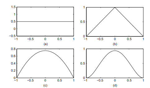
In order to shift the distribution $F_{X}$ of a random variable $X$ a distortion function $g$ is applied to the cumulative distribution function $F_{X}$. Such function $g$ is defined on $[0,1] \rightarrow[0 ; 1]$ such that $g(0)=0$ and $g(1)=1$, and is a continuous increasing function (Wang and Young 1998; Wang 2000).
Distortion functions arose from empirical observations that people do not evaluate risk as a linear function of the actual probabilities for different outcomes but rather as a nonlinear distortion function. It is used to transform the probabilities of the loss distribution to another probability distribution by re-weighting the original distribution. This transformation increases the weight given to desirable events and deflates others. Different distortions $g$ have been proposed in the literature. Some functions are provided in Table $4.1$, where the parameters $k$ and $\gamma$ represent the confidence level and the level of risk aversion.
When $g$ is a concave function, its first derivative $g^{\prime}$ is an increasing function, $g^{\prime}\left(S_{X}(x)\right)$ where $S_{X}=P[X>x]$ is a decreasing function ${ }^{1}$ in $x$ and $g^{\prime}\left(S_{X}(x)\right)$ represents a weighted coefficient which discounts the probability of desirable events while loading the probability of adverse events. A first approach for the distortion operator is $g_{\alpha}(u)=\Phi\left[\Phi^{-1}(u)+\alpha\right]$, where $\Phi$ is the Gaussian cumulative distribution. In terms of risk measure this last function applies the same perspective of preference to quantify the risk associated with gain and risk. Thus, a risk manager evaluates the risk associated with the upside and downside risks with the same function $g$ implying a symmetric consideration for the two effects due to the
distortion. Moreover it induces the same confidence level for the losses and the gain which implies the same level of risk aversion associated with the losses and the gains.
In Fig. $4.3$ the impact on the logistic distribution of the previous distortion function introduced is presented. We remark that the distorted distribution is always symmetrical under this kind of distortion function, and we observe a shift in the mode of the initial distribution towards the left.
To avoid the problem of symmetry, the following distortion function can be used: $g_{i}(u)=u+k_{i}\left(u-u^{2}\right)$ for $\left.\left.k \in\right] 0,1\right]$ et $\forall i \in{1,2}$. In a risk measure perspective one models losses and gains differently relatively to the values of the parameters $k_{i}, i=$ 1,2 . Thus upside and downside risks are modelled in different ways. Nevertheless the calibration of the parameters $k_{i}, i=1,2$ is not easy.
量化风险管理代考
金融代写|量化风险管理代写Quantitative Risk Management代考|Examples of Parametric Distributions
椭圆分布:这类分布包括高斯分布和吨-分配。
- 随机变量X如果它的密度(平均μ和方差σ2) 是这样的
FX(X)=1(2圆周率)1/2σ经验(−12σ2(X−μ)−2).
这种分布是对称的,并且非常迅速地向零下降。什么时候μ=0和σ=1,则其峰度等于 3 。该值用作基准来确定任何分布是否具有低尾行为(峰度小于 3 )或高尾行为(峰度大于 3 )。 - 这吨-分布密度与:
FX(X)=11+(X2/ν)(在+1)/2.
这吨-分布的尾巴变得更重在增加(在是自由度数)。这种分布在金融中并不容易使用,因为在parameter 是一个整数,而不是一个连续的参数,限制了它的使用灵活性。 - 可以使用其他分布,其性质与前两个分布互补,因为它们具有更多参数。在金融领域,我们对具有高峰度的重尾分布函数感兴趣,因为它更容易出现极端值。例如,可以考虑 GED 分布。归一化为均值为零且方差为 1 的 GED 随机变量的密度由下式给出:
$$
f(z)=\frac{\operatorname{vexp}\left[-1 /\left.2|| _{\lambda}\right|^{v}\right]}{\lambda 2^{1+1 / v} \Gamma(1 / v)},-\infty2,吨H和d一世s吨r一世b在吨一世○n○F和H一个s吨H一世nn和r吨一个一世ls吨H一个n吨H和n○r米一个l.吨H一世sd和ns一世吨是一个pp和一个rs米○r和pr和F和r一个bl和吨○吨H和小号吨在d和n吨−吨d一世s吨r一世b在吨一世○nb和C一个在s和v \in R^{+}$。
金融代写|量化风险管理代写Quantitative Risk Management代考|Non-parametric Modelling for a Distribution
非参数设置避免了参数密度选择的不确定性,并允许限制由于用于估计密度参数的估计程序而导致的误差(Silverman 2018)。
假设给定独立的同分布实值观测(X1,⋯,Xn)有密度F. 我们估计F在点的网格上X1,⋯,X米, 对于任何任意米固定的,特别是在这里,我们专注于单点估计X. 如果F在一个小街区很顺利[X−H,X+H]的X,可以得到以下近似:
2H⋅F(X)≈∫X−HX+HF(在)d在=磷(X∈[X−H,X+H])
由中值定理。(4.1.14) 的右边可以通过计算X一世的在长度的小区间内2H,然后除以n. 这是一个带有 bincentre 的直方图估计器X和带宽2H. 让ķ(在)= 12我(|在|≤1), 在哪里我(.)是指示函数,当事件为真时取值为 1,否则取值为 0。然后,直方图估计量可以写成:
F^H(X)=n−1∑一世=1nķH(X−X一世)
在哪里ķH(.)=H−1ķH(./H). 表达式 (4.1.15) 称为核密度估计F(X)带内核ķ(在)=12我(|在|≤1)和带宽H.
阶跃函数内核对窗口内的每个观察值进行平均加权,即使观察值更接近X应该拥有比更远的信息更好的信息。此外,阶跃函数估计器在X,考虑到平滑度假设,这是没有吸引力的F. 这两个目标都可以通过选择更平滑的“窗口函数”来满足ķ作为内核,即一个ķ(在)→0 为|在|→1. 核是一个分段连续函数,围绕零对称,积分为一:
ķ(在)=ķ(−在);∫ķ(在)d在=1.
金融代写|量化风险管理代写Quantitative Risk Management代考|Shift of a Distribution
为了改变分布FX随机变量X失真函数G应用于累积分布函数FX. 这样的功能G定义在[0,1]→[0;1]这样G(0)=0和G(1)=1,并且是一个连续递增的函数(Wang and Young 1998;Wang 2000)。
失真函数源于经验观察,即人们不会将风险评估为不同结果的实际概率的线性函数,而是作为非线性失真函数。它用于通过重新加权原始分布将损失分布的概率转换为另一个概率分布。这种转变增加了对理想事件的权重,并降低了其他事件的权重。不同的扭曲G已在文献中提出。表中提供了一些功能4.1, 其中参数ķ和C代表置信水平和风险厌恶程度。
什么时候G是凹函数,它的一阶导数G′是一个增函数,G′(小号X(X))在哪里小号X=磷[X>X]是一个递减函数1在X和G′(小号X(X))表示一个加权系数,它在加载不良事件概率的同时,对期望事件的概率进行折现。失真算子的第一种方法是G一个(在)=披[披−1(在)+一个], 在哪里披是高斯累积分布。在风险度量方面,最后一个函数应用相同的偏好视角来量化与收益和风险相关的风险。因此,风险经理使用相同的功能评估与上行和下行风险相关的风险G意味着对这两种效应进行对称考虑,因为
失真。此外,它对损失和收益产生相同的置信水平,这意味着与损失和收益相关的风险厌恶程度相同。
在图。4.3介绍了之前引入的失真函数对逻辑分布的影响。我们注意到在这种失真函数下,失真分布总是对称的,并且我们观察到初始分布的模式向左移动。
为了避免对称性问题,可以使用以下失真函数:G一世(在)=在+ķ一世(在−在2)为了ķ∈]0,1]和∀一世∈1,2. 从风险度量的角度来看,一个模型的损失和收益相对于参数的值是不同的ķ一世,一世=1,2 。因此,上行和下行风险以不同的方式建模。尽管如此,参数的校准ķ一世,一世=1,2不简单。

统计代写请认准statistics-lab™. statistics-lab™为您的留学生涯保驾护航。
金融工程代写
金融工程是使用数学技术来解决金融问题。金融工程使用计算机科学、统计学、经济学和应用数学领域的工具和知识来解决当前的金融问题,以及设计新的和创新的金融产品。
非参数统计代写
非参数统计指的是一种统计方法,其中不假设数据来自于由少数参数决定的规定模型;这种模型的例子包括正态分布模型和线性回归模型。
广义线性模型代考
广义线性模型(GLM)归属统计学领域,是一种应用灵活的线性回归模型。该模型允许因变量的偏差分布有除了正态分布之外的其它分布。
术语 广义线性模型(GLM)通常是指给定连续和/或分类预测因素的连续响应变量的常规线性回归模型。它包括多元线性回归,以及方差分析和方差分析(仅含固定效应)。
有限元方法代写
有限元方法(FEM)是一种流行的方法,用于数值解决工程和数学建模中出现的微分方程。典型的问题领域包括结构分析、传热、流体流动、质量运输和电磁势等传统领域。
有限元是一种通用的数值方法,用于解决两个或三个空间变量的偏微分方程(即一些边界值问题)。为了解决一个问题,有限元将一个大系统细分为更小、更简单的部分,称为有限元。这是通过在空间维度上的特定空间离散化来实现的,它是通过构建对象的网格来实现的:用于求解的数值域,它有有限数量的点。边界值问题的有限元方法表述最终导致一个代数方程组。该方法在域上对未知函数进行逼近。[1] 然后将模拟这些有限元的简单方程组合成一个更大的方程系统,以模拟整个问题。然后,有限元通过变化微积分使相关的误差函数最小化来逼近一个解决方案。
tatistics-lab作为专业的留学生服务机构,多年来已为美国、英国、加拿大、澳洲等留学热门地的学生提供专业的学术服务,包括但不限于Essay代写,Assignment代写,Dissertation代写,Report代写,小组作业代写,Proposal代写,Paper代写,Presentation代写,计算机作业代写,论文修改和润色,网课代做,exam代考等等。写作范围涵盖高中,本科,研究生等海外留学全阶段,辐射金融,经济学,会计学,审计学,管理学等全球99%专业科目。写作团队既有专业英语母语作者,也有海外名校硕博留学生,每位写作老师都拥有过硬的语言能力,专业的学科背景和学术写作经验。我们承诺100%原创,100%专业,100%准时,100%满意。
随机分析代写
随机微积分是数学的一个分支,对随机过程进行操作。它允许为随机过程的积分定义一个关于随机过程的一致的积分理论。这个领域是由日本数学家伊藤清在第二次世界大战期间创建并开始的。
时间序列分析代写
随机过程,是依赖于参数的一组随机变量的全体,参数通常是时间。 随机变量是随机现象的数量表现,其时间序列是一组按照时间发生先后顺序进行排列的数据点序列。通常一组时间序列的时间间隔为一恒定值(如1秒,5分钟,12小时,7天,1年),因此时间序列可以作为离散时间数据进行分析处理。研究时间序列数据的意义在于现实中,往往需要研究某个事物其随时间发展变化的规律。这就需要通过研究该事物过去发展的历史记录,以得到其自身发展的规律。
回归分析代写
多元回归分析渐进(Multiple Regression Analysis Asymptotics)属于计量经济学领域,主要是一种数学上的统计分析方法,可以分析复杂情况下各影响因素的数学关系,在自然科学、社会和经济学等多个领域内应用广泛。
MATLAB代写
MATLAB 是一种用于技术计算的高性能语言。它将计算、可视化和编程集成在一个易于使用的环境中,其中问题和解决方案以熟悉的数学符号表示。典型用途包括:数学和计算算法开发建模、仿真和原型制作数据分析、探索和可视化科学和工程图形应用程序开发,包括图形用户界面构建MATLAB 是一个交互式系统,其基本数据元素是一个不需要维度的数组。这使您可以解决许多技术计算问题,尤其是那些具有矩阵和向量公式的问题,而只需用 C 或 Fortran 等标量非交互式语言编写程序所需的时间的一小部分。MATLAB 名称代表矩阵实验室。MATLAB 最初的编写目的是提供对由 LINPACK 和 EISPACK 项目开发的矩阵软件的轻松访问,这两个项目共同代表了矩阵计算软件的最新技术。MATLAB 经过多年的发展,得到了许多用户的投入。在大学环境中,它是数学、工程和科学入门和高级课程的标准教学工具。在工业领域,MATLAB 是高效研究、开发和分析的首选工具。MATLAB 具有一系列称为工具箱的特定于应用程序的解决方案。对于大多数 MATLAB 用户来说非常重要,工具箱允许您学习和应用专业技术。工具箱是 MATLAB 函数(M 文件)的综合集合,可扩展 MATLAB 环境以解决特定类别的问题。可用工具箱的领域包括信号处理、控制系统、神经网络、模糊逻辑、小波、仿真等。