如果你也在 怎样代写随机偏微分方程这个学科遇到相关的难题,请随时右上角联系我们的24/7代写客服。
随机偏微分方程通过随机力项和系数来概括偏微分方程。
研究最多的SPDEs之一是随机热方程,它可以正式写为
$$
\partial_{t} u=\Delta u+\xi,
$$
statistics-lab™ 为您的留学生涯保驾护航 在代写随机偏微分方程方面已经树立了自己的口碑, 保证靠谱, 高质且原创的统计Statistics代写服务。我们的专家在代写随机偏微分方程代写方面经验极为丰富,各种代写随机偏微分方程相关的作业也就用不着说。
我们提供的随机偏微分方程及其相关学科的代写,服务范围广, 其中包括但不限于:
- Statistical Inference 统计推断
- Statistical Computing 统计计算
- Advanced Probability Theory 高等概率论
- Advanced Mathematical Statistics 高等数理统计学
- (Generalized) Linear Models 广义线性模型
- Statistical Machine Learning 统计机器学习
- Longitudinal Data Analysis 纵向数据分析
- Foundations of Data Science 数据科学基础
金融代写|随机偏微分方程代写Stochastic partial differential equations代考|Meta Theorems
The first result presented here is the attractivity. It justifies the scaling of ansatz (1.4) used for the formal derivation. It heavily relies on the structure of the equation. Sometimes we rely on global nonlinear stability and sometimes we only use linear stability on the non-dominant modes. A typical statement would be:
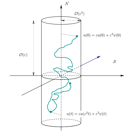
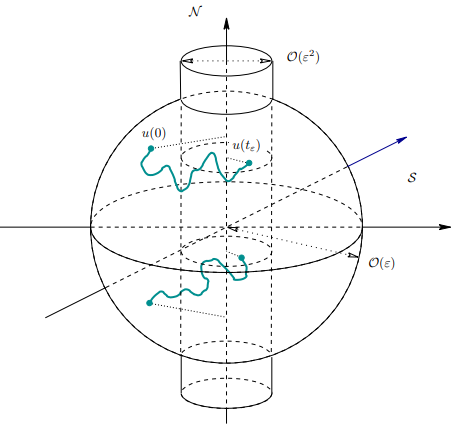
Theorem 1.1 (Attractivity) There is a time $t_{e}=\mathcal{O}\left(\ln \left(\varepsilon^{-1}\right)\right)$ such that for all solutions $u$ of (1.19) with initial conditions $u(0)$ of order $\mathcal{O}(\varepsilon)$ we have $u_{s}\left(t_{e}\right)=$ $\mathcal{O}\left(\varepsilon^{2}\right)$ and $u_{c}\left(t_{e}\right)=\mathcal{O}(\varepsilon)$. This means the solution looks at the time $t_{e}$ like ansatz (1.4). To be more precise $u\left(t_{\varepsilon}\right)=\varepsilon a_{e}+\varepsilon^{2} \psi_{\varepsilon}$ with $a_{\varepsilon} \in \mathcal{N}$ and $\psi_{e} \in \mathcal{S}$ both of order $\mathcal{O}(1)$.
If we assume additionally global nonlinear stability for the equation, then there is a time $T_{\varepsilon}=\mathcal{O}\left(\varepsilon^{-2}\right)$ such that $u\left(T_{\varepsilon}\right)=\mathcal{O}(\varepsilon)$ independent of the initial condition.
This theorem is rigorously stated in Theorems $2.7$ or $2.8$. We will give a detailed discussion of these results for multiplicative noise in Theorems $2.1$ and $2.4$ for cubic and quadratic nonlinearities. A sketch of the typical dynamics for the local attractivity result is given in Figure 1.3.
Remark 1.4 Depending on the assumptions the statement $g_{e}=\mathcal{O}\left(f_{\varepsilon}\right)$ can have two different meanings. Depending on the context, we either use that for all $p>0$ there is a constant $C>0$ such that $\mathbb{E}\left|g_{e}\right|^{p} \leq C f_{\varepsilon}^{p}$ for all $\varepsilon \in(0,1]$. This is typically
only valid for nonlinear stable equations, where we can actually bound moments. In case of, for instance quadratic nonlinearities, where in general we do not have control on moments of solutions, we also use the somewhat weaker meaning that for some constant $C>0$, we have $\mathbb{P}\left(\left|g_{\varepsilon}\right| \geq C f_{\varepsilon}\right)$ uniformly small for all $\varepsilon \in(0,1]$. Sometimes we also give explicit convergence rates of this probability for $\varepsilon \rightarrow 0$.
For a solution $a$ of $(1.5)$ and $\psi$ of (1.6) we define first the approximations $\varepsilon w_{k}$ of order $k$ by
$$
\varepsilon w_{1}(t):=\varepsilon a\left(\varepsilon^{2} t\right) \text { and } \varepsilon w_{2}(t):=\varepsilon a\left(\varepsilon^{2} t\right)+\varepsilon^{2} \psi(t)
$$
In our setting the residual of $\varepsilon w$ is defined by
$$
\begin{aligned}
\operatorname{Res}(\varepsilon w)(t)=&-\varepsilon w(t)+\mathrm{e}^{t L} \varepsilon w(0)+\varepsilon^{2} W_{L}(t) \
&+\int_{0}^{t} \mathrm{e}^{(t-\tau) L}\left\varepsilon^{3} A w+\mathcal{F}(\varepsilon w)\right d \tau
\end{aligned}
$$
金融代写|随机偏微分方程代写Stochastic partial differential equations代考|Examples of Equations
In the literature there are numerous examples of equations where the abstract theorems do apply. In this section we focus mainly on additive noise. For instance, for cubic nonlinearities the well known Ginzburg-Landau equation (see [DE00] for a standard proof of existence of unique solutions)
$$
\partial_{t} u=\Delta u+\nu u-u^{3}+\sigma \xi
$$
and the Swift-Hohenberg equation (see [CH93] for numerous references)
$$
\partial_{t} u=-(\Delta+1)^{2} u+\nu u-u^{3}+\sigma \xi
$$
fall into the scope of our work, in case the parameters $\nu$ and $\sigma$ are small and of comparable order of magnitude. Both equations are considered on bounded domains with suitable boundary conditions (e.g. periodic, Dirichlet, Neumann, etc.). The Swift-Hohenberg equation is a toy model for the convective instability in the Rayleigh-Bénard convection. A formal derivation of the equation from the Boussinesq approximation of fluid dynamics can be found in [SH77].
Another example arising in the theory of surface growth is
$$
\partial_{t} u=-\Delta^{2} u-\mu \Delta u+\nabla \cdot\left(|\nabla u|^{2} \nabla u\right)+\sigma \xi,
$$
subject to periodic boundary conditions and moving frame $\int_{G} u d x=0$, where one rescales the mean growth of $u$ out of the equation, in order to ensure a Poincare type inequality. This model was first suggested by [LDS91]. The deterministic equation was rigorously treated in [KSW03]. For a review on surface growth see for example [BS95] or [HHZ95]. For this model we can consider $\mu=\mu_{0}+\varepsilon^{2}$ and $\sigma=\mathcal{O}\left(\varepsilon^{2}\right)$,where $\mu_{0}$ is such that $L=-\Delta^{2} u-\mu_{0} \Delta u$ is a non-positive operator with non-zero kernel. We will see later on, that all examples presented up to now exhibit a stable nonlinearity in the sense of Assumption 2.2.
金融代写|随机偏微分方程代写Stochastic partial differential equations代考|Bounded Domains
On bounded domains, we can approximate on long time-scales the essential dynamics of an SPDE near a change of stability by the amplitude equation. This is in this chapter just an SDE describing the dynamics of the dominating modes, which are the ones that change sign in the linearisation. For the formal derivation in the case of additive noise see Sections 1.1.1 or 1.1.3. The main mathematical reason why the other modes are not important is the presence of a well defined spectral gap in the linearised equation of order $\mathcal{O}(1)$ between the eigenvalues of the dominant eigenfunctions and the remainder of the spectrum.
The approximation via SDE is only meaningful for small domains. If the domain gets larger, one needs very small noise to apply the results. See Chapter 4 , where the size of the domain is coupled to the distance from bifurcation. Problems arise due to the fact that, if we enlarge the domain, then we shrink the spectral gap. The precise definition of the spectral gap $\omega$ will be given in Assumption 2.1. The main problem is that a lot of constants depend on $\omega$, and they tend to infinity for $\omega \rightarrow 0$. But if the domain-size $\ell \rightarrow \infty$, then in most cases $\omega \rightarrow 0$. Hence, for large domains our result is only meaningful for very small noise strength $\varepsilon^{2}$ with $\varepsilon \in\left(0, \varepsilon_{0}\right]$, where $\varepsilon_{0}=\varepsilon_{0}(\ell) \rightarrow 0$ for $\ell \rightarrow \infty$. However, the linear part of our equation is usually coupled to the noise, and thus has to be very small, too. The main problem is now, that this linear part reflects the influence of control parameters adjusted in experiments. It is not possible to consider it arbitrarily small.
In the following, we demonstrate the power of our approach by applying it to PDEs perturbed by a simple multiplicative noise. Although our results apply to more complicated noise terms, for simplicity of presentation we consider only this very simple example in order to outline the main ideas in a less technical way. The results for additive noise are reviewed later in this chapter.
随机偏微分方程代写
金融代写|随机偏微分方程代写Stochastic partial differential equations代考|Meta Theorems
这里展示的第一个结果是吸引力。它证明了用于形式推导的 ansatz (1.4) 的缩放比例。它在很大程度上依赖于方程的结构。有时我们依赖全局非线性稳定性,有时我们只对非主模使用线性稳定性。一个典型的陈述是:
定理 1.1(吸引力)有一段时间吨和=这(ln(e−1))这样对于所有解决方案在(1.19)的初始条件在(0)有秩序的这(e)我们有在s(吨和)= 这(e2)和在C(吨和)=这(e). 这意味着解决方案着眼于时间吨和像 ansatz (1.4)。更准确地说在(吨e)=e一种和+e2ψe和一种e∈ñ和ψ和∈小号两个顺序这(1).
如果我们另外假设方程的全局非线性稳定性,那么有一个时间吨e=这(e−2)这样在(吨e)=这(e)独立于初始条件。
这个定理在 Theorems 中有严格的表述2.7或者2.8. 我们将在定理中详细讨论乘性噪声的这些结果2.1和2.4对于三次和二次非线性。图 1.3 给出了局部吸引力结果的典型动力学示意图。
备注 1.4 根据假设,陈述G和=这(Fe)可以有两种不同的含义。根据上下文,我们要么将其用于所有p>0有一个常数C>0这样和|G和|p≤CFep对全部e∈(0,1]. 这通常是
仅对非线性稳定方程有效,我们实际上可以约束矩。例如,在二次非线性的情况下,通常我们无法控制解的矩,我们也使用较弱的含义,即对于某些常数C>0, 我们有磷(|Ge|≥CFe)对所有人都一样小e∈(0,1]. 有时我们也给出这个概率的显式收敛率e→0.
寻求解决方案一种的(1.5)和ψ(1.6)我们首先定义近似值e在ķ有秩序的ķ经过
e在1(吨):=e一种(e2吨) 和 e在2(吨):=e一种(e2吨)+e2ψ(吨)
在我们的设置中,残差e在定义为
$$
\begin{aligned}
\operatorname{Res}(\varepsilon w)(t)=&-\varepsilon w(t)+\mathrm{e}^{t L} \varepsilon w(0)+ \varepsilon^{2} W_{L}(t) \
&+\int_{0}^{t} \mathrm{e}^{(t-\tau) L}\left \varepsilon^{3} A w+ \mathcal{F}(\varepsilon w)\right d \tau
\end{aligned}
$$
金融代写|随机偏微分方程代写Stochastic partial differential equations代考|Examples of Equations
在文献中有许多应用抽象定理的方程的例子。在本节中,我们主要关注加性噪声。例如,对于三次非线性,众所周知的 Ginzburg-Landau 方程(有关唯一解存在的标准证明,请参见 [DE00])
∂吨在=Δ在+ν在−在3+σX
和 Swift-Hohenberg 方程(参见 [CH93] 以获取大量参考资料)
∂吨在=−(Δ+1)2在+ν在−在3+σX
属于我们的工作范围,以防参数ν和σ很小并且具有可比的数量级。两个方程都考虑在具有合适边界条件的有界域上(例如,周期性、Dirichlet、Neumann 等)。Swift-Hohenberg 方程是 Rayleigh-Bénard 对流中对流不稳定性的玩具模型。可以在 [SH77] 中找到从流体动力学的 Boussinesq 近似对方程的正式推导。
表面生长理论中出现的另一个例子是
∂吨在=−Δ2在−μΔ在+∇⋅(|∇在|2∇在)+σX,
受周期性边界条件和移动框架的影响∫G在dX=0,其中重新调整平均增长在出方程,以确保 Poincare 类型的不等式。该模型首先由 [LDS91] 提出。[KSW03] 中严格处理了确定性方程。有关表面生长的评论,请参见例如 [BS95] 或 [HHZ95]。对于这个模型,我们可以考虑μ=μ0+e2和σ=这(e2),在哪里μ0是这样的大号=−Δ2在−μ0Δ在是具有非零内核的非正算子。稍后我们将看到,到目前为止提出的所有示例都表现出假设 2.2 意义上的稳定非线性。
金融代写|随机偏微分方程代写Stochastic partial differential equations代考|Bounded Domains
在有界域上,我们可以通过幅度方程在长时间尺度上近似 SPDE 在稳定性变化附近的基本动力学。在本章中,这只是一个描述主要模式动态的 SDE,它们是在线性化中改变符号的模式。对于加性噪声情况下的形式推导,请参见第 1.1.1 或 1.1.3 节。其他模式不重要的主要数学原因是线性化阶方程中存在明确定义的光谱间隙这(1)在主要特征函数的特征值和谱的其余部分之间。
通过 SDE 进行的近似仅对小域有意义。如果域变大,则需要非常小的噪声来应用结果。请参阅第 4 章,其中域的大小与分岔的距离有关。问题出现的原因是,如果我们扩大域,那么我们会缩小光谱间隙。光谱间隙的精确定义ω将在假设 2.1 中给出。主要问题是很多常量依赖于ω,并且它们趋向于无穷大ω→0. 但是如果域大小ℓ→∞, 那么在大多数情况下ω→0. 因此,对于大域,我们的结果仅对非常小的噪声强度有意义e2和e∈(0,e0], 在哪里e0=e0(ℓ)→0为了ℓ→∞. 然而,我们方程的线性部分通常与噪声耦合,因此也必须非常小。现在的主要问题是,这个线性部分反映了实验中调整的控制参数的影响。不可能认为它任意小。
在下文中,我们通过将其应用于受简单乘性噪声干扰的 PDE 来展示我们方法的强大功能。尽管我们的结果适用于更复杂的噪声项,但为了简单起见,我们只考虑这个非常简单的示例,以便以不太技术性的方式概述主要思想。本章稍后将回顾加性噪声的结果。

统计代写请认准statistics-lab™. statistics-lab™为您的留学生涯保驾护航。
金融工程代写
金融工程是使用数学技术来解决金融问题。金融工程使用计算机科学、统计学、经济学和应用数学领域的工具和知识来解决当前的金融问题,以及设计新的和创新的金融产品。
非参数统计代写
非参数统计指的是一种统计方法,其中不假设数据来自于由少数参数决定的规定模型;这种模型的例子包括正态分布模型和线性回归模型。
广义线性模型代考
广义线性模型(GLM)归属统计学领域,是一种应用灵活的线性回归模型。该模型允许因变量的偏差分布有除了正态分布之外的其它分布。
术语 广义线性模型(GLM)通常是指给定连续和/或分类预测因素的连续响应变量的常规线性回归模型。它包括多元线性回归,以及方差分析和方差分析(仅含固定效应)。
有限元方法代写
有限元方法(FEM)是一种流行的方法,用于数值解决工程和数学建模中出现的微分方程。典型的问题领域包括结构分析、传热、流体流动、质量运输和电磁势等传统领域。
有限元是一种通用的数值方法,用于解决两个或三个空间变量的偏微分方程(即一些边界值问题)。为了解决一个问题,有限元将一个大系统细分为更小、更简单的部分,称为有限元。这是通过在空间维度上的特定空间离散化来实现的,它是通过构建对象的网格来实现的:用于求解的数值域,它有有限数量的点。边界值问题的有限元方法表述最终导致一个代数方程组。该方法在域上对未知函数进行逼近。[1] 然后将模拟这些有限元的简单方程组合成一个更大的方程系统,以模拟整个问题。然后,有限元通过变化微积分使相关的误差函数最小化来逼近一个解决方案。
tatistics-lab作为专业的留学生服务机构,多年来已为美国、英国、加拿大、澳洲等留学热门地的学生提供专业的学术服务,包括但不限于Essay代写,Assignment代写,Dissertation代写,Report代写,小组作业代写,Proposal代写,Paper代写,Presentation代写,计算机作业代写,论文修改和润色,网课代做,exam代考等等。写作范围涵盖高中,本科,研究生等海外留学全阶段,辐射金融,经济学,会计学,审计学,管理学等全球99%专业科目。写作团队既有专业英语母语作者,也有海外名校硕博留学生,每位写作老师都拥有过硬的语言能力,专业的学科背景和学术写作经验。我们承诺100%原创,100%专业,100%准时,100%满意。
随机分析代写
随机微积分是数学的一个分支,对随机过程进行操作。它允许为随机过程的积分定义一个关于随机过程的一致的积分理论。这个领域是由日本数学家伊藤清在第二次世界大战期间创建并开始的。
时间序列分析代写
随机过程,是依赖于参数的一组随机变量的全体,参数通常是时间。 随机变量是随机现象的数量表现,其时间序列是一组按照时间发生先后顺序进行排列的数据点序列。通常一组时间序列的时间间隔为一恒定值(如1秒,5分钟,12小时,7天,1年),因此时间序列可以作为离散时间数据进行分析处理。研究时间序列数据的意义在于现实中,往往需要研究某个事物其随时间发展变化的规律。这就需要通过研究该事物过去发展的历史记录,以得到其自身发展的规律。
回归分析代写
多元回归分析渐进(Multiple Regression Analysis Asymptotics)属于计量经济学领域,主要是一种数学上的统计分析方法,可以分析复杂情况下各影响因素的数学关系,在自然科学、社会和经济学等多个领域内应用广泛。
MATLAB代写
MATLAB 是一种用于技术计算的高性能语言。它将计算、可视化和编程集成在一个易于使用的环境中,其中问题和解决方案以熟悉的数学符号表示。典型用途包括:数学和计算算法开发建模、仿真和原型制作数据分析、探索和可视化科学和工程图形应用程序开发,包括图形用户界面构建MATLAB 是一个交互式系统,其基本数据元素是一个不需要维度的数组。这使您可以解决许多技术计算问题,尤其是那些具有矩阵和向量公式的问题,而只需用 C 或 Fortran 等标量非交互式语言编写程序所需的时间的一小部分。MATLAB 名称代表矩阵实验室。MATLAB 最初的编写目的是提供对由 LINPACK 和 EISPACK 项目开发的矩阵软件的轻松访问,这两个项目共同代表了矩阵计算软件的最新技术。MATLAB 经过多年的发展,得到了许多用户的投入。在大学环境中,它是数学、工程和科学入门和高级课程的标准教学工具。在工业领域,MATLAB 是高效研究、开发和分析的首选工具。MATLAB 具有一系列称为工具箱的特定于应用程序的解决方案。对于大多数 MATLAB 用户来说非常重要,工具箱允许您学习和应用专业技术。工具箱是 MATLAB 函数(M 文件)的综合集合,可扩展 MATLAB 环境以解决特定类别的问题。可用工具箱的领域包括信号处理、控制系统、神经网络、模糊逻辑、小波、仿真等。