如果你也在 怎样代写随机偏微分方程这个学科遇到相关的难题，请随时右上角联系我们的24/7代写客服。

随机偏微分方程通过随机力项和系数来概括偏微分方程。

研究最多的SPDEs之一是随机热方程，它可以正式写为
$$
\partial_{t} u=\Delta u+\xi,
$$

statistics-lab™ 为您的留学生涯保驾护航 在代写随机偏微分方程方面已经树立了自己的口碑, 保证靠谱, 高质且原创的统计Statistics代写服务。我们的专家在代写随机偏微分方程代写方面经验极为丰富，各种代写随机偏微分方程相关的作业也就用不着说。

我们提供的随机偏微分方程及其相关学科的代写，服务范围广, 其中包括但不限于:

• Statistical Inference 统计推断
• Statistical Computing 统计计算
• Advanced Probability Theory 高等概率论
• Advanced Mathematical Statistics 高等数理统计学
• (Generalized) Linear Models 广义线性模型
• Statistical Machine Learning 统计机器学习
• Longitudinal Data Analysis 纵向数据分析
• Foundations of Data Science 数据科学基础

金融代写|随机偏微分方程代写Stochastic partial differential equations代考|Approximative Centre Manifold

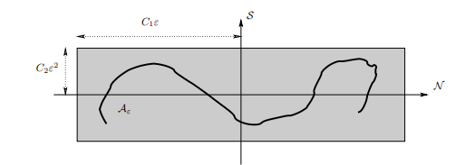
This section describes how the evolution of solutions of a stochastic PDE subject to additive forcing is determined by an approximate centre manifold. This was briefly discussed in [Blö03] for the first order approximation. There the manifold is just

the vector space $\mathcal{N}$. It attracts solutions up to errors of order $\mathcal{O}\left(\varepsilon^{2}\right)$, and the flow along $\mathcal{N}$ is given on the slow time-scale by the amplitude equation.

Here, we first state the results of Section $4.1$ in [BH05], which relies on the second order correction introduced in [BH04] to describe the distance from $\mathcal{N}$, too. Therefore we need nonlinear stability, in order to bound moments. That is why we restrict ourselves in the following to nonlinear stable equations given by Assumption $2.7$.

The key difference from results on random invariant manifolds (cf. for example [DLS03] or [MZZ07; DLS04; DW06b]) is that we obtain in first order $\mathcal{O}(\varepsilon)$ a fixed object, instead of a random set that is moving in time. Our result allows to control this dynamics at least to order $\mathcal{O}\left(\varepsilon^{2}\right)$ or $\mathcal{O}\left(\varepsilon^{3}\right)$. We pay for that qualitative description, by having all statements just with high probability, and not almost surely.

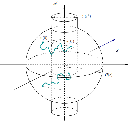
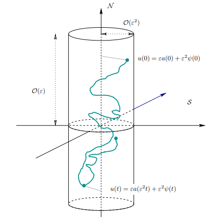
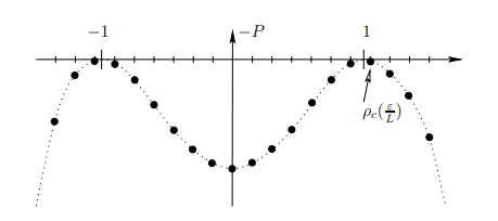
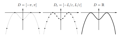
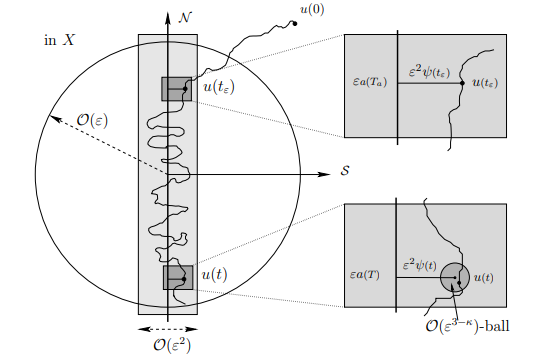
Our main result shows that in first order the flow of solutions of the SPDE (1.2) along $\mathcal{N}$ is well approximated by $\varepsilon a\left(\varepsilon^{2} t\right)$, where $a$ is the solution of the amplitude equation. In second order $\mathcal{O}\left(\varepsilon^{2}\right)$, the distance from $\mathcal{N}$ is given by fast oscillations, which is given as a stationary Ornstein-Uhlenbeck process $\varepsilon^{2} \psi^{\star}(t)$. Thus the solutions are attracted by an $\mathcal{O}\left(\varepsilon^{3-\kappa}\right)$-neighbourhood of $\varepsilon^{2} \psi^{\star}(t)+\mathcal{N}$. Note that everything is valid only with high probability. Note that the setting for multiplicative noise is simpler, as the deterministic fixed point 0 is available. Therefore local results on the structure of invariant manifolds were obtained much earlier in that case (cf. for example [CLR01]). In Figure $3.2$ the typical behaviour of solutions is given.

金融代写|随机偏微分方程代写Stochastic partial differential equations代考|Random Fixed Points

Let us discuss the dynamics of random fixed points for random dynamical systems induced by the SPDE. At this point we do not give a precise definition of random dynamical systems (see [Arn98] for details) or random fixed points (see for example [Sch98]). In this section it is enough to know that a random fixed point induces a stationary solution for the SPDE, if we start the SPDE in the random fixed point.
Theorem 3.7 Suppose Assumptions 2.5, 2.7, and $2.8$ are true, and let $u^{}(t)$ be a stationary mild solution in $X$ of (1.2). Let a be the solution of (1.5) with $a(0)=\varepsilon^{-1} P_{c} u^{}(0)$. Furthermore let $\psi^{\star}$ be the stationary Ornstein-Uhlenbeck given by (3.25).

Then there is a constant $c_{0}>0$ such that for all $T_{0}>0$ any small $\kappa \in(0,1)$, and all $p \geq 1$, there exists a constant $C>0$, such that
$$
\mathbb{E}\left(\sup {t \in\left[c{0} \ln (1 / \varepsilon), T_{0} / \varepsilon^{2}\right]}\left|u^{}(t)-\varepsilon a\left(t \varepsilon^{2}\right)-\varepsilon^{2} \psi^{\star}(t)\right|_{X}^{p}\right)^{1 / p} \leq C \varepsilon^{3-\kappa} . $$ This result is an extension of the result for invariant measures (cf. Theorem 3.1), as the law of the stationary solution is at a fixed time $t$ exactly an invariant measure. Here we can control the time-evolution, too. Idea of proof: First we start the approximation result with initial condition $u^{}\left(-T_{a} \varepsilon^{-2}\right)$ for some $T_{a}>0$. This implies first for $t=0$, but then due to stationarity for all $t$, that
$$
\left(\mathbb{E}\left|u^{}(t)\right|^{p}\right)^{1 / p} \leq C \varepsilon \quad \text { and } \quad\left(\mathbb{E}\left|P_{s} u^{}(t)\right|^{p}\right)^{1 / p} \leq C \varepsilon^{2} .
$$
Thus, we can start the approximation result in 0 . and get
$$
\mathbb{E}\left(\sup {t \in\left[0, T{0} / \varepsilon^{2}\right]}\left|u^{}(t)-\varepsilon a\left(t \varepsilon^{2}\right)-\varepsilon^{2} \psi(t)\right|_{X}^{p}\right)^{1 / p} \leq C \varepsilon^{3-\kappa}, $$ where $\psi$ is the OU-process with initial condition $\psi(0)=\varepsilon^{-2} P_{s} u^{}(0)$.
After a time scale of oder $\mathcal{O}(\ln (1 / \varepsilon))$ we can approximate $\psi$ with $\psi^{}$ as $$ \psi(t)=\mathrm{e}^{t L}\left(\psi(0)-\psi^{}(0)\right)+\psi^{*}(t)
$$

金融代写|随机偏微分方程代写Stochastic partial differential equations代考|Random Set Attractors

Let us extend our result for random fixed points (cf. Section 3.3.1) to random attractors. We do not present the result in full detail, but rather focus on a brief description of all steps necessary. Most steps are just quite technical but straightforward extensions of the estimates necessary for the residual, attractivity, and approximation. The key point is to rely on path-wise estimates, and take expectations in the end.
Assumption 3.3 Consider eq. (1.2) fulfilling Assumptions 2.5, 2.7, and 2.8.
The main example, we keep in mind is the stochastic Swift-Hohenberg equation in the space $X=L^{2}(G)$.

First we can use standard a priori estimates relying on nonlinear stability. This is very similar to Theorem $2.8$, but nevertheless, we need to get uniform bounds with respect to the initial conditions
$$
u(0) \in B_{r}:={x \in X:|x| \leq r}
$$
for any fixed $r>0$. For this we establish path-wise bounds for $v=u-\varepsilon^{2} \phi$ with $\phi=W_{L-\varepsilon^{2}}$, which solves the following random PDE (compare (2.87))
$$
\partial_{t} v=L v+\varepsilon^{2}(A v+\phi)+\varepsilon^{4} A \phi+\mathcal{F}\left(v+\varepsilon^{2} \phi\right), \quad v(0)=u(0) .
$$
We use standard deterministic a priori estimates for (3.26), and take expectations in the end. Note that this transformation is not ergodic, in contrast to the usual transformation in the theory of random attractors, where one uses the stationary Ornstein-Uhlenbeck process for $\phi$. For our setting we rely on $\phi$, as we do not want to change initial conditions in (3.26).

The first step is the attractivity. It is similar to the proof of Theorem $2.8$ and follows from standard a priori estimates for $v$ and the stochastic convolution. Note that we rely on nonlinear stability. The result is that for all $r>0$ there is a time $T_{e}=\mathcal{O}\left(\varepsilon^{-2}\right)$ such that for all $p>0$
$$
\mathbb{E}\left(\sup {u(0) \in B{r}}|u(t)|^{p}\right) \leq C \varepsilon^{p} \text { for all } t \geq T_{e} .
$$

随机偏微分方程代写

金融代写|随机偏微分方程代写Stochastic partial differential equations代考|Approximative Centre Manifold

本节描述了受加性强迫影响的随机 PDE 解的演化如何由近似中心流形确定。这在 [Blö03] 中针对一阶近似进行了简要讨论。那里的歧管只是

向量空间ñ. 它吸引解决订单错误的解决方案这(e2), 和流动ñ由振幅方程在慢时间尺度上给出。

在这里，我们首先陈述一下Section的结果4.1在[BH05]中，它依赖于[BH04]中引入的二阶校正来描述距离ñ， 也。因此，我们需要非线性稳定性，以便约束矩。这就是为什么我们将自己限制在以下由假设给出的非线性稳定方程2.7.

与随机不变流形上的结果（参见例如 [DLS03] 或 [MZZ07; DLS04; DW06b]）的主要区别在于我们在一阶获得这(e)一个固定的对象，而不是随时间移动的随机集合。我们的结果允许至少控制这种动态这(e2)或者这(e3). 我们为这种定性描述付出了代价，因为所有陈述都具有很高的概率，而不是几乎肯定。

我们的主要结果表明，在一阶 SPDE (1.2) 的解流沿着ñ很好地近似于e一种(e2吨)， 在哪里一种是幅度方程的解。在二阶这(e2), 距离ñ由快速振荡给出，它被给出为一个平稳的 Ornstein-Uhlenbeck 过程e2ψ⋆(吨). 因此，解决方案被吸引这(e3−ķ)- 邻里e2ψ⋆(吨)+ñ. 请注意，一切只有在高概率下才有效。请注意，乘性噪声的设置更简单，因为确定性固定点 0 可用。因此，在这种情况下更早地获得了关于不变流形结构的局部结果（参见例如 [CLR01]）。如图3.2给出了解决方案的典型行为。

金融代写|随机偏微分方程代写Stochastic partial differential equations代考|Random Fixed Points

让我们讨论由 SPDE 引起的随机动力系统的随机不动点的动力学。在这一点上，我们没有给出随机动力系统（详见[Arn98]）或随机固定点（参见例如[Sch98]）的精确定义。在本节中，如果我们在随机不动点中启动 SPDE，则只要知道随机不动点会导致 SPDE 的平稳解就足够了。
定理 3.7 假设假设 2.5、2.7 和2.8是真的，并且让在(吨)是一个平稳的温和溶液X(1.2)。设 a 为 (1.5) 的解一种(0)=e−1磷C在(0). 此外让ψ⋆是由 (3.25) 给出的静止 Ornstein-Uhlenbeck。

然后有一个常数C0>0这样对于所有人吨0>0任何小的ķ∈(0,1)， 和所有p≥1, 存在一个常数C>0, 这样
和(支持吨∈[C0ln⁡(1/e),吨0/e2]|在(吨)−e一种(吨e2)−e2ψ⋆(吨)|Xp)1/p≤Ce3−ķ.该结果是不变测度结果的扩展（参见定理 3.1），因为固定解的定律在固定时间吨完全是一个不变的度量。在这里，我们也可以控制时间演化。证明思路：首先我们以初始条件开始逼近结果在(−吨一种e−2)对于一些吨一种>0. 这意味着首先对于吨=0, 但是由于所有的平稳性吨， 那
(和|在(吨)|p)1/p≤Ce 和 (和|磷s在(吨)|p)1/p≤Ce2.
因此，我们可以从 0 开始近似结果。并得到
和(支持吨∈[0,吨0/e2]|在(吨)−e一种(吨e2)−e2ψ(吨)|Xp)1/p≤Ce3−ķ,在哪里ψ是具有初始条件的 OU 过程ψ(0)=e−2磷s在(0).
经过一段时间的订单这(ln⁡(1/e))我们可以近似ψ和ψ作为ψ(吨)=和吨大号(ψ(0)−ψ(0))+ψ∗(吨)

金融代写|随机偏微分方程代写Stochastic partial differential equations代考|Random Set Attractors

让我们将随机固定点的结果（参见第 3.3.1 节）扩展到随机吸引子。我们不会详细介绍结果，而是专注于对所有必要步骤的简要描述。大多数步骤只是对残差、吸引力和近似所必需的估计的技术性但直接的扩展。关键是要依靠路径估计，并最终取得预期。
假设 3.3 考虑等式。(1.2) 满足假设 2.5、2.7 和 2.8。
我们记住的主要例子是空间中的随机 Swift-Hohenberg 方程X=大号2(G).

首先，我们可以使用依赖于非线性稳定性的标准先验估计。这与定理非常相似2.8，但是，我们需要得到关于初始条件的统一界限
在(0)∈乙r:=X∈X:|X|≤r
对于任何固定r>0. 为此，我们为在=在−e2φ和φ=在大号−e2，它解决了以下随机 PDE（比较 (2.87)）
∂吨在=大号在+e2(一种在+φ)+e4一种φ+F(在+e2φ),在(0)=在(0).
我们对 (3.26) 使用标准确定性先验估计，并最终采用期望值。请注意，这种变换不是遍历的，与随机吸引子理论中的通常变换相反，后者使用平稳​​的 Ornstein-Uhlenbeck 过程φ. 对于我们的设置，我们依赖φ，因为我们不想改变（3.26）中的初始条件。

第一步是吸引力。类似于定理的证明2.8并遵循标准的先验估计在和随机卷积。请注意，我们依赖非线性稳定性。结果是所有人r>0有一段时间吨和=这(e−2)这样对于所有人p>0
和(支持在(0)∈乙r|在(吨)|p)≤Cep 对全部 吨≥吨和.

统计代写请认准statistics-lab™. statistics-lab™为您的留学生涯保驾护航。

金融工程代写

金融工程是使用数学技术来解决金融问题。金融工程使用计算机科学、统计学、经济学和应用数学领域的工具和知识来解决当前的金融问题，以及设计新的和创新的金融产品。

非参数统计代写

非参数统计指的是一种统计方法，其中不假设数据来自于由少数参数决定的规定模型；这种模型的例子包括正态分布模型和线性回归模型。

广义线性模型代考

广义线性模型（GLM）归属统计学领域，是一种应用灵活的线性回归模型。该模型允许因变量的偏差分布有除了正态分布之外的其它分布。

术语 广义线性模型（GLM）通常是指给定连续和/或分类预测因素的连续响应变量的常规线性回归模型。它包括多元线性回归，以及方差分析和方差分析（仅含固定效应）。

有限元方法代写

有限元方法（FEM）是一种流行的方法，用于数值解决工程和数学建模中出现的微分方程。典型的问题领域包括结构分析、传热、流体流动、质量运输和电磁势等传统领域。

有限元是一种通用的数值方法，用于解决两个或三个空间变量的偏微分方程（即一些边界值问题）。为了解决一个问题，有限元将一个大系统细分为更小、更简单的部分，称为有限元。这是通过在空间维度上的特定空间离散化来实现的，它是通过构建对象的网格来实现的：用于求解的数值域，它有有限数量的点。边界值问题的有限元方法表述最终导致一个代数方程组。该方法在域上对未知函数进行逼近。[1] 然后将模拟这些有限元的简单方程组合成一个更大的方程系统，以模拟整个问题。然后，有限元通过变化微积分使相关的误差函数最小化来逼近一个解决方案。

tatistics-lab作为专业的留学生服务机构，多年来已为美国、英国、加拿大、澳洲等留学热门地的学生提供专业的学术服务，包括但不限于Essay代写，Assignment代写，Dissertation代写，Report代写，小组作业代写，Proposal代写，Paper代写，Presentation代写，计算机作业代写，论文修改和润色，网课代做，exam代考等等。写作范围涵盖高中，本科，研究生等海外留学全阶段，辐射金融，经济学，会计学，审计学，管理学等全球99%专业科目。写作团队既有专业英语母语作者，也有海外名校硕博留学生，每位写作老师都拥有过硬的语言能力，专业的学科背景和学术写作经验。我们承诺100%原创，100%专业，100%准时，100%满意。

随机分析代写

随机微积分是数学的一个分支，对随机过程进行操作。它允许为随机过程的积分定义一个关于随机过程的一致的积分理论。这个领域是由日本数学家伊藤清在第二次世界大战期间创建并开始的。

时间序列分析代写

随机过程，是依赖于参数的一组随机变量的全体，参数通常是时间。 随机变量是随机现象的数量表现，其时间序列是一组按照时间发生先后顺序进行排列的数据点序列。通常一组时间序列的时间间隔为一恒定值（如1秒，5分钟，12小时，7天，1年），因此时间序列可以作为离散时间数据进行分析处理。研究时间序列数据的意义在于现实中，往往需要研究某个事物其随时间发展变化的规律。这就需要通过研究该事物过去发展的历史记录，以得到其自身发展的规律。

回归分析代写

多元回归分析渐进（Multiple Regression Analysis Asymptotics）属于计量经济学领域，主要是一种数学上的统计分析方法，可以分析复杂情况下各影响因素的数学关系，在自然科学、社会和经济学等多个领域内应用广泛。

MATLAB代写

MATLAB 是一种用于技术计算的高性能语言。它将计算、可视化和编程集成在一个易于使用的环境中，其中问题和解决方案以熟悉的数学符号表示。典型用途包括：数学和计算算法开发建模、仿真和原型制作数据分析、探索和可视化科学和工程图形应用程序开发，包括图形用户界面构建MATLAB 是一个交互式系统，其基本数据元素是一个不需要维度的数组。这使您可以解决许多技术计算问题，尤其是那些具有矩阵和向量公式的问题，而只需用 C 或 Fortran 等标量非交互式语言编写程序所需的时间的一小部分。MATLAB 名称代表矩阵实验室。MATLAB 最初的编写目的是提供对由 LINPACK 和 EISPACK 项目开发的矩阵软件的轻松访问，这两个项目共同代表了矩阵计算软件的最新技术。MATLAB 经过多年的发展，得到了许多用户的投入。在大学环境中，它是数学、工程和科学入门和高级课程的标准教学工具。在工业领域，MATLAB 是高效研究、开发和分析的首选工具。MATLAB 具有一系列称为工具箱的特定于应用程序的解决方案。对于大多数 MATLAB 用户来说非常重要，工具箱允许您学习和应用专业技术。工具箱是 MATLAB 函数（M 文件）的综合集合，可扩展 MATLAB 环境以解决特定类别的问题。可用工具箱的领域包括信号处理、控制系统、神经网络、模糊逻辑、小波、仿真等。

R语言代写	问卷设计与分析代写
PYTHON代写	回归分析与线性模型代写
MATLAB代写	方差分析与试验设计代写
STATA代写	机器学习/统计学习代写
SPSS代写	计量经济学代写
EVIEWS代写	时间序列分析代写
EXCEL代写	深度学习代写
SQL代写	各种数据建模与可视化代写

如果你也在 怎样代写随机偏微分方程这个学科遇到相关的难题，请随时右上角联系我们的24/7代写客服。

随机偏微分方程通过随机力项和系数来概括偏微分方程。

研究最多的SPDEs之一是随机热方程，它可以正式写为
$$
\partial_{t} u=\Delta u+\xi,
$$

statistics-lab™ 为您的留学生涯保驾护航 在代写随机偏微分方程方面已经树立了自己的口碑, 保证靠谱, 高质且原创的统计Statistics代写服务。我们的专家在代写随机偏微分方程代写方面经验极为丰富，各种代写随机偏微分方程相关的作业也就用不着说。

我们提供的随机偏微分方程及其相关学科的代写，服务范围广, 其中包括但不限于:

• Statistical Inference 统计推断
• Statistical Computing 统计计算
• Advanced Probability Theory 高等概率论
• Advanced Mathematical Statistics 高等数理统计学
• (Generalized) Linear Models 广义线性模型
• Statistical Machine Learning 统计机器学习
• Longitudinal Data Analysis 纵向数据分析
• Foundations of Data Science 数据科学基础

金融代写|随机偏微分方程代写Stochastic partial differential equations代考|Some Examples

This chapter presents applications of the approximation via amplitude equations. The main results are about long-time behaviour of SPDEs or transient pattern formation for SPDEs on bounded domains. For simplicity of presentation, we focus on a few examples, in order to highlight the key ideas.

By no means we give an exhaustive presentation of all results possible, but focus on three examples. First we treat approximation of invariant measures near a change of stability. This is a review of results of [BH04]. We give the main ideas without stating details of the proofs.

The second section on pattern formation below threshold of instability gives a self-contained introduction, by explaining ideas and giving all proofs in the simplest setting possible. The final section on approximative centre manifolds and approximation of random attractors gives only the main ideas of proofs.
Invariant Measures
Section $3.1$ states the approximation of invariant measures for the corresponding dual Markov semigroup. We summarise some of the results of [BH04]. Near the change of stability the invariant measure is well described in first order of $\varepsilon$ by the invariant measure of the amplitude equation plus in second order by an infinite dimensional Ornstein-Uhlenbeck measure on the stable modes $\mathcal{S}$. The result is of the type $\mathbb{P}^{u^{}}=\mathbb{P}^{e a^{}} \otimes \mathbb{P}^{e^{2} \psi^{*}}$. In this part the presentation is based on the setting and the results of Section 2.5. Apart from large deviation results, this is the first rigorous qualitative result for the structure of invariant measures for SPDEs with additive noise.

Another interesting application, that we nevertheless do not treat here, is the discussion of phenomenological bifurcation for SPDEs. It relies on the approximation of invariant measures. The invariant measure in $\mathcal{N}$ for the amplitude equation is usually easy to describe. For instance one can use the celebrated Fokker-Planck equation (cf. Risken [Ris84]), where we identify $\mathcal{N}$ with some $\mathbb{R}^{n}$ with $n \in{1,2}$ for many examples. The Fokker-Planck equation is a deterministic PDE, which solution provides a smooth Lebesgue density of invariant measures on $\mathcal{N}$.

金融代写|随机偏微分方程代写Stochastic partial differential equations代考|Approximation of Invariant Measures

This section reviews the results obtained in [BH04] on approximating the invariant measure of SPDEs of the type of (1.2) near a change of stability. For simplicity the result is based on the setting of Section 2.5, where we considered a stable cubic nonlinearity and additive noise. To be more precise, consider equation (1.2) and let Assumptions 2.5, 2.7, and $2.8$ be true. Additive noise is important, in order to have a unique exponential attracting invariant measure for the amplitude equation (cf. Assumption $3.1$ and the discussion below).

It is a main issue to have the speed of convergence to the invariant measure for the amplitude equations under control (see (3.7)). The flow has to be (up to small errors) a contraction on the space of probability measures. This makes multiplicative noise more complicated, as there could be more than one invariant measure, and the speed of convergence is not controlled, as even nearby initial conditions may converge to different measures. A similar problem arises, when the amplitude equation is deterministic, for example, if the noise strength in the SPDE is $\mathcal{O}\left(\varepsilon^{3}\right)$. Here only partial results are available. Again problems arise with the speed of convergence in the amplitude equation, once its deterministic attractor is not trivial.

金融代写|随机偏微分方程代写Stochastic partial differential equations代考|The Results

Before we state our results, we introduce one more notation. For simplicity of presentation, we rescale the solutions of (1.2) by $\varepsilon$ such that they are concentrated on a set of order 1 instead of a set of order $\varepsilon$. Furthermore, we rescale the equation to the slow time-scale $T=t \varepsilon^{2}$. Thus we consider $v$ given by $v(T)=\varepsilon^{-1} u\left(T \varepsilon^{-2}\right)$, where we split as usual $v=v_{c}+v_{s}\left(v_{c} \in \mathcal{N}, v_{s} \in \mathcal{S}\right)$. We obtain
$$
\begin{array}{lc}
\partial_{T} v_{c}= & A_{c}\left(v_{c}+v_{s}\right)+\mathcal{F}{c}\left(v{c}+v_{s}\right)+\partial_{T} \beta \
\partial_{T} v_{s}=\varepsilon^{-2} L v_{s}+A_{s}\left(v_{c}+v_{s}\right)+\mathcal{F}{s}\left(v{c}+v_{s}\right)+\partial_{T} \hat{W}{s} \end{array} $$ where $\hat{W}{s}(T)=\varepsilon P_{s} Q W\left(\varepsilon^{-2} T\right)$ and $\beta(T)=\varepsilon P_{c} Q W\left(\varepsilon^{-2} T\right)$, as usual.
We denote by $\mu_{\star}^{e}$ an invariant measure of (3.4). Note that the existence is standard using the celebrated Krylov-Bogoliubov method (cf. [DPZ96]).

Definition 3.5 Denote by $\nu_{\star}^{}$ the invariant measure for the pair of processes $(a, \varepsilon \psi)$, where the evolution is given by $(1.5)$ and (1.6). Hence, in the slow time variable $$ \begin{aligned} &\partial_{T} a=A_{c} a+\mathcal{F}{c}(a)+\partial{T} \beta \
&\partial_{T} \psi=\varepsilon^{-2} L \psi+\partial_{T} \hat{W}{s} \end{aligned} $$ Denote by $\nu{\star}^{c}$ the marginal on $\mathcal{N}$, and by $\nu_{\star}^{s}$ the one on $\mathcal{S}$, respectively.
Note that we actually do not need the uniqueness of $\nu_{\star}^{}$. We only need that the marginals on $\mathcal{N}$ and $\mathcal{S}$ are unique. The uniqueness of $\nu_{\star}^{s}$ is obvious, as we have an Ornstein-Uhlenbeck process. Furthermore, the uniqueness of $\nu_{\star}^{c}$ follows from Assumption 3.1.

Note that $\nu_{\star}^{*}$ depends on $\varepsilon$ by the rescaling of $\psi$. Recall also that we discussed in Remark $2.8$ that the two noise terms in (3.5) may not be independent. Thus the equations in (3.5) are coupled through the noise, but actually they do not live on the same time scale, as the second equation in (3.5) lives on the fast time-scale $t$. However, as the equations are otherwise decoupled, we can determine the marginals $\nu_{\star}^{c}$ and $\nu_{\star}^{s}$ independently. The marginal $\nu_{\star}^{\mathrm{c}}$ is independent of $\varepsilon$ and $\nu_{\star}^{s}$ depends on $\varepsilon$ only through the trivial scaling of $\varepsilon \psi$. Therefore we suppressed this $\varepsilon$-dependence in the notation.

With these notations, our main result in the Wasserstein distance is the following.

随机偏微分方程代写

金融代写|随机偏微分方程代写Stochastic partial differential equations代考|Some Examples

本章介绍通过幅度方程进行近似的应用。主要结果是关于 SPDE 的长期行为或 SPDE 在有界域上的瞬态模式形成。为简单起见，我们将重点放在几个示例上，以突出关键思想。

我们绝不会对所有可能的结果进行详尽的介绍，而是关注三个示例。首先，我们处理接近稳定性变化的不变测度的近似。这是对[BH04]结果的回顾。我们给出了主要思想，但没有说明证明的细节。

关于低于不稳定阈值的模式形成的第二部分给出了一个独立的介绍，通过解释想法并在最简单的设置中给出所有证明。关于近似中心流形和随机吸引子近似的最后一节仅给出了证明的主要思想。
不变测量
部分3.1陈述了对应的对偶马尔可夫半群的不变测度的近似。我们总结了[BH04]的一些结果。在稳定性变化附近，不变测度在第一阶中得到了很好的描述e通过振幅方程的不变测量加上二阶对稳定模式的无限维 Ornstein-Uhlenbeck 测量小号. 结果的类型为 $\mathbb{P}^{u^{ }}=\mathbb{P}^{ea^{ }} \otimes \mathbb{P}^{e^{2} \psi^{ *}}$。在这部分中，演示基于第 2.5 节的设置和结果。除了较大的偏差结果外，这是具有加性噪声的 SPDE 的不变测度结构的第一个严格的定性结果。

另一个有趣的应用，我们在这里不讨论，是对 SPDE 的现象学分岔的讨论。它依赖于不变测度的近似。不变测度ñ因为幅度方程通常很容易描述。例如，我们可以使用著名的 Fokker-Planck 方程（参见 Risken [Ris84]），我们确定ñ和一些Rn和n∈1,2举很多例子。Fokker-Planck 方程是一个确定性 PDE，它提供了一个平滑的 Lebesgue 密度的不变测度ñ.

金融代写|随机偏微分方程代写Stochastic partial differential equations代考|Approximation of Invariant Measures

本节回顾在 [BH04] 中获得的关于在稳定性变化附近近似 (1.2) 类型的 SPDE 的不变测度的结果。为简单起见，结果基于第 2.5 节的设置，其中我们考虑了稳定的三次非线性和加性噪声。更准确地说，考虑方程 (1.2) 并让假设 2.5、2.7 和2.8是真的。加性噪声很重要，以便对幅度方程具有独特的指数吸引不变测量（参见假设3.1以及下面的讨论）。

控制幅度方程的不变测度的收敛速度是一个主要问题（见（3.7））。流量必须是（直到小错误）概率度量空间的收缩。这使得乘性噪声变得更加复杂，因为可能存在不止一个不变测度，并且收敛速度不受控制，因为即使是附近的初始条件也可能会收敛到不同的测度。当幅度方程是确定的时，也会出现类似的问题，例如，如果 SPDE 中的噪声强度为这(e3). 这里只有部分结果可用。振幅方程的收敛速度再次出现问题，一旦它的确定性吸引子不是微不足道的。

金融代写|随机偏微分方程代写Stochastic partial differential equations代考|The Results

在我们陈述我们的结果之前，我们再介绍一种符号。为简单起见，我们重新调整（1.2）的解决方案e这样它们就集中在一组订单 1 而不是一组订单e. 此外，我们将方程重新缩放到慢时间尺度吨=吨e2. 因此我们认为在由在(吨)=e−1在(吨e−2), 我们像往常一样分裂在=在C+在s(在C∈ñ,在s∈小号). 我们得到
$$
\begin{array}{lc}
\partial_{T} v_{c}= & A_{c}\left(v_{c}+v_{s}\right)+\mathcal{F} {c }\left(v {c}+v_{s}\right)+\partial_{T} \beta \
\partial_{T} v_{s}=\varepsilon^{-2} L v_{s}+A_{ s}\left(v_{c}+v_{s}\right)+\mathcal{F} {s}\left(v {c}+v_{s}\right)+\partial_{T} \hat{ W} {s} \end{array} $$ 其中 $\hat{W} {s}(T)=\varepsilon P_{s} QW\left(\varepsilon^{-2} T\right)一种nd\beta(T)=\varepsilon P_{c} QW\left(\varepsilon^{-2} T\right),一种s在s在一种l.在和d和n这吨和b是\mu_{\star}^{e}$ (3.4) 的不变测度。请注意，存在是使用著名的 Krylov-Bogoliubov 方法（参见 [DPZ96]）的标准。

定义 3.5 表示为ν⋆过程对的不变测度(一种,eψ)，其中进化由下式给出(1.5)和 (1.6)。因此，在慢时间变量∂吨一种=一种C一种+FC(一种)+∂吨b ∂吨ψ=e−2大号ψ+∂吨在^s表示为ν⋆C边际上ñ，并由ν⋆s那个在小号， 分别。
请注意，我们实际上并不需要唯一性ν⋆. 我们只需要ñ和小号是独一无二的。的独特性ν⋆s很明显，因为我们有一个 Ornstein-Uhlenbeck 过程。此外，它的独特性ν⋆C遵循假设 3.1。

注意ν⋆∗取决于e通过重新调整ψ. 还记得我们在备注中讨论过的2.8（3.5）中的两个噪声项可能不是独立的。因此（3.5）中的方程通过噪声耦合，但实际上它们并不存在于相同的时间尺度上，因为（3.5）中的第二个方程存在于快速时间尺度上吨. 然而，由于方程是解耦的，我们可以确定边缘ν⋆C和ν⋆s独立。边缘的ν⋆C独立于e和ν⋆s取决于e只有通过微不足道的缩放eψ. 因此我们压制了这个e-符号中的依赖性。

使用这些符号，我们在 Wasserstein 距离中的主要结果如下。

统计代写请认准statistics-lab™. statistics-lab™为您的留学生涯保驾护航。

金融工程代写

金融工程是使用数学技术来解决金融问题。金融工程使用计算机科学、统计学、经济学和应用数学领域的工具和知识来解决当前的金融问题，以及设计新的和创新的金融产品。

非参数统计代写

非参数统计指的是一种统计方法，其中不假设数据来自于由少数参数决定的规定模型；这种模型的例子包括正态分布模型和线性回归模型。

广义线性模型代考

广义线性模型（GLM）归属统计学领域，是一种应用灵活的线性回归模型。该模型允许因变量的偏差分布有除了正态分布之外的其它分布。

术语 广义线性模型（GLM）通常是指给定连续和/或分类预测因素的连续响应变量的常规线性回归模型。它包括多元线性回归，以及方差分析和方差分析（仅含固定效应）。

有限元方法代写

有限元方法（FEM）是一种流行的方法，用于数值解决工程和数学建模中出现的微分方程。典型的问题领域包括结构分析、传热、流体流动、质量运输和电磁势等传统领域。

有限元是一种通用的数值方法，用于解决两个或三个空间变量的偏微分方程（即一些边界值问题）。为了解决一个问题，有限元将一个大系统细分为更小、更简单的部分，称为有限元。这是通过在空间维度上的特定空间离散化来实现的，它是通过构建对象的网格来实现的：用于求解的数值域，它有有限数量的点。边界值问题的有限元方法表述最终导致一个代数方程组。该方法在域上对未知函数进行逼近。[1] 然后将模拟这些有限元的简单方程组合成一个更大的方程系统，以模拟整个问题。然后，有限元通过变化微积分使相关的误差函数最小化来逼近一个解决方案。

tatistics-lab作为专业的留学生服务机构，多年来已为美国、英国、加拿大、澳洲等留学热门地的学生提供专业的学术服务，包括但不限于Essay代写，Assignment代写，Dissertation代写，Report代写，小组作业代写，Proposal代写，Paper代写，Presentation代写，计算机作业代写，论文修改和润色，网课代做，exam代考等等。写作范围涵盖高中，本科，研究生等海外留学全阶段，辐射金融，经济学，会计学，审计学，管理学等全球99%专业科目。写作团队既有专业英语母语作者，也有海外名校硕博留学生，每位写作老师都拥有过硬的语言能力，专业的学科背景和学术写作经验。我们承诺100%原创，100%专业，100%准时，100%满意。

随机分析代写

随机微积分是数学的一个分支，对随机过程进行操作。它允许为随机过程的积分定义一个关于随机过程的一致的积分理论。这个领域是由日本数学家伊藤清在第二次世界大战期间创建并开始的。

时间序列分析代写

随机过程，是依赖于参数的一组随机变量的全体，参数通常是时间。 随机变量是随机现象的数量表现，其时间序列是一组按照时间发生先后顺序进行排列的数据点序列。通常一组时间序列的时间间隔为一恒定值（如1秒，5分钟，12小时，7天，1年），因此时间序列可以作为离散时间数据进行分析处理。研究时间序列数据的意义在于现实中，往往需要研究某个事物其随时间发展变化的规律。这就需要通过研究该事物过去发展的历史记录，以得到其自身发展的规律。

回归分析代写

多元回归分析渐进（Multiple Regression Analysis Asymptotics）属于计量经济学领域，主要是一种数学上的统计分析方法，可以分析复杂情况下各影响因素的数学关系，在自然科学、社会和经济学等多个领域内应用广泛。

MATLAB代写

MATLAB 是一种用于技术计算的高性能语言。它将计算、可视化和编程集成在一个易于使用的环境中，其中问题和解决方案以熟悉的数学符号表示。典型用途包括：数学和计算算法开发建模、仿真和原型制作数据分析、探索和可视化科学和工程图形应用程序开发，包括图形用户界面构建MATLAB 是一个交互式系统，其基本数据元素是一个不需要维度的数组。这使您可以解决许多技术计算问题，尤其是那些具有矩阵和向量公式的问题，而只需用 C 或 Fortran 等标量非交互式语言编写程序所需的时间的一小部分。MATLAB 名称代表矩阵实验室。MATLAB 最初的编写目的是提供对由 LINPACK 和 EISPACK 项目开发的矩阵软件的轻松访问，这两个项目共同代表了矩阵计算软件的最新技术。MATLAB 经过多年的发展，得到了许多用户的投入。在大学环境中，它是数学、工程和科学入门和高级课程的标准教学工具。在工业领域，MATLAB 是高效研究、开发和分析的首选工具。MATLAB 具有一系列称为工具箱的特定于应用程序的解决方案。对于大多数 MATLAB 用户来说非常重要，工具箱允许您学习和应用专业技术。工具箱是 MATLAB 函数（M 文件）的综合集合，可扩展 MATLAB 环境以解决特定类别的问题。可用工具箱的领域包括信号处理、控制系统、神经网络、模糊逻辑、小波、仿真等。

R语言代写	问卷设计与分析代写
PYTHON代写	回归分析与线性模型代写
MATLAB代写	方差分析与试验设计代写
STATA代写	机器学习/统计学习代写
SPSS代写	计量经济学代写
EVIEWS代写	时间序列分析代写
EXCEL代写	深度学习代写
SQL代写	各种数据建模与可视化代写

如果你也在 怎样代写随机偏微分方程这个学科遇到相关的难题，请随时右上角联系我们的24/7代写客服。

随机偏微分方程通过随机力项和系数来概括偏微分方程。

研究最多的SPDEs之一是随机热方程，它可以正式写为
$$
\partial_{t} u=\Delta u+\xi,
$$

statistics-lab™ 为您的留学生涯保驾护航 在代写随机偏微分方程方面已经树立了自己的口碑, 保证靠谱, 高质且原创的统计Statistics代写服务。我们的专家在代写随机偏微分方程代写方面经验极为丰富，各种代写随机偏微分方程相关的作业也就用不着说。

我们提供的随机偏微分方程及其相关学科的代写，服务范围广, 其中包括但不限于:

• Statistical Inference 统计推断
• Statistical Computing 统计计算
• Advanced Probability Theory 高等概率论
• Advanced Mathematical Statistics 高等数理统计学
• (Generalized) Linear Models 广义线性模型
• Statistical Machine Learning 统计机器学习
• Longitudinal Data Analysis 纵向数据分析
• Foundations of Data Science 数据科学基础

金融代写|随机偏微分方程代写Stochastic partial differential equations代考|Assumptions

Let us summarise all assumptions necessary for our results. We do not focus on the highest possible level of generality, but stick to some simpler setting which cover all our examples. First consider the linear operator $L$.

Assumption 2.5 Let $X$ be a separable Hilbert space and $\Delta$ (subject to some boundary conditions on a bounded domain) be a self-adjoint version of the Laplacian on $X$. Suppose $L=P(-\Delta)$ for some function $P$ such that $L$ is non-positive. Furthermore, let the kernel $\mathcal{N}=\operatorname{ker} L$ of $L$ be non-empty and finite dimensional. Finally, suppose $P(k) \rightarrow-\infty$ as $k \rightarrow \infty$.

This assumption is a stronger than the one in Section 2.2. It is mainly used for convenience of presentation, and covers all examples presented. Furthermore, it is just a special case of Assumption 2.1, and in the following we can use all the implications of this assumption. We use the notation $P_{c}$ and $P_{s}$, which are in this case just the standard orthogonal projections. Additionally, recall the splitting $X=\mathcal{N} \oplus \mathcal{S}$ with $\mathcal{S}=P_{s} X$ and the spaces $X^{\alpha}$ from Section 2.2. Recall furthermore the bounds (2.4), (2.5), and (2.6) for the analytic semigroup $\mathrm{e}^{t L}$ generated by $L$.
For the nonlinearities, we make two assumptions. The first one, is much weaker than Assumption 2.2, as we are aiming only for local results in that case. Especially, we can get rid of the strong nonlinear dissipativity. The second assumption is similar to Assumption $2.2$ and involves strong nonlinear stability and dissipativity conditions in $\mathcal{N}$.

Assumption 2.6 The function $\mathcal{F}$ is locally Lipschitz from $X$ to $X^{-\alpha}$ for some $\alpha \in[0,1)$. This means that for all $R>0$ there is a $C>0$ such that
$$
\left|\mathcal{F}\left(v_{1}\right)-\mathcal{F}\left(v_{2}\right)\right|_{-\alpha} \leq C\left|v_{1}-v_{2}\right| \quad \text { for all } v_{i} \text { with }\left|v_{i}\right| \leq R
$$
Assume we can split $\mathcal{F}(x)=f(x)+g(x)$, where $f: X \times X \times X \rightarrow X^{-\alpha}$ is continuous, trilinear, and symmetric. The function $g$ is of higher order, which means $|g(x)|_{-\alpha} \leq C|x|^{4}$ provided $|x| \leq 1 .$

金融代写|随机偏微分方程代写Stochastic partial differential equations代考|Amplitude Equations Main Results

Theorem 2.7 (Attractivity-local) Under Assumptions $2.5,2.6$, and $2.8$ fix some small constant $\kappa>0$. Then there are constants $c_{i}>0$ and a time $t_{e}=$ $\mathcal{O}\left(\ln \left(\varepsilon^{-1}\right)\right)$ such that for all mild solutions $u$ of $(2.86)$ we can write
$$
u\left(t_{e}\right)=\varepsilon a_{e}+\varepsilon^{2} R_{e} \quad \text { with } \quad a_{\varepsilon} \in \mathcal{N} \text { and } R_{e} \in \mathcal{S}
$$
where
$$
\mathbb{P}\left(\left|a_{e}\right| \leq \delta,|R e| \leq \varepsilon^{-\kappa}\right) \geq \mathbb{P}\left(|u(0)| \leq c_{3} \delta \varepsilon\right)-c_{1} e^{-c_{2} e^{-2 \kappa}}
$$
for all $\delta>1$ and $\varepsilon \in(0,1)$.
This result states in a weak form that $u(0)=\mathcal{O}(\varepsilon)$ with high probability implies $P_{c} u\left(t_{\varepsilon}\right)=\mathcal{O}(\varepsilon)$ and $P_{s} u\left(t_{\varepsilon}\right)=\mathcal{O}\left(\varepsilon^{2}\right)$ with high probability, too. Note that we do not bound any moments of the solution $u$.

We do not give a detailed proof of this result, as it is a straightforward modification of Theorem $3.3$ of [Blö03]. It relies on the fact that small solutions of order $\mathcal{O}(\varepsilon)$ are on small time-scales given by the linearised picture, which is dominated by the semigroup estimates $(2.5)$ and $(2.6)$. Thus modes in $P_{s} X$ decay exponentially fast on a time-scale of order $\mathcal{O}(1)$.
Using strong nonlinear stability, we can prove much more:
Theorem 2.8 (Attractivity-global) Let Assumptions 2.5, 2.6, and 2.8 be satisfied. Then for all times $T_{e}=T_{0} \varepsilon^{-2}>0$ and for all $p \geq 1$ there are constants $C_{p}>0$ explicitly depending on $p$ such that
$$
\mathbb{E}\left|u\left(t+T_{e}\right)\right|^{p} \leq C_{p} \varepsilon^{p} \quad \text { and } \quad \mathbb{E}\left|P_{s} u\left(t+T_{e}\right)\right|^{p} \leq C_{p} \varepsilon^{2 p}
$$
for all $t \geq 0$, all $X$-valued mild solutions $u$ of equation (1.2) independent of the initial condition $u(0)$, and for all $\varepsilon \in(0,1)$.

Furthermore, if we already assume that $\mathbb{E}|u(0)|{ }^{p} \leq C_{p} \varepsilon^{p}$ for a constant $C_{p}>0$, then there is a time $t_{\varepsilon}=\mathcal{O}\left(\ln \left(\varepsilon^{-1}\right)\right)$ and a constant $C>0$ such that
$$
\mathbb{E}|u(t)|^{p} \leq C \varepsilon^{p} \quad \text { and } \quad \mathbb{E}\left|P_{s} u\left(t+t_{e}\right)\right|^{p} \leq C \varepsilon^{2 p}
$$
for all $t \geq 0$, all $X$-valued mild solutions $u$, and for all $\varepsilon \in(0,1)$.
The proof is given by a priori estimates. This was not directly proved in [BH04], but under our somewhat stronger assumptions this is similar to Lemma $4.3$ of [BH04]. It relies on a priori estimates for $v_{\delta_{\varepsilon}}=u-\varepsilon^{2} W_{L-\delta_{c}}$ with $\delta_{e}=\mathcal{O}\left(\varepsilon^{2}\right)$, which fulfils a random PDE similar to $(2.87)$. The main technical advantage is that the linear semigroup generated by $L-\delta_{e}$ is exponentially stable.
2.5.3.2 Approximation
For a solution $a$ of $(1.5)$ and $\psi$ of $(1.6)$ we define the approximations $\varepsilon w_{k}$ of order $k$ by
$$
\varepsilon w_{1}(t):=\varepsilon a\left(\varepsilon^{2} t\right) \text { and } \varepsilon w_{2}(t):=\varepsilon a\left(\varepsilon^{2} t\right)+\varepsilon^{2} \psi(t)
$$

金融代写|随机偏微分方程代写Stochastic partial differential equations代考|Quadratic Nonlinearities

In this section we review the results of [Blö05a]. Consider an SPDE of the following type.
$$
\partial_{t} u=L u+\varepsilon^{2} A u+B(u, u)+\varepsilon^{2} \xi
$$
where $L$ as in Assumption 2.1. The linear operator $A$ and the bilinear operator $B$ are as in Assumption 2.4, and the noise is the generalised derivative of some Wiener process (cf. Assumption 2.9).

In [Blö05a] we used fractional noise. This was motivated by the fact that the proofs rely on fractional integration by parts formulas, and explicit path-wise estimates. Here we state for simplicity only the version for Gaussian noise that is white in time. Note that due to the method of proof, we need the noise to be trace-class, as we need bounds for the Wiener process $W(t)$ in the space $X$. This obviously rules out space-time white noise.

Let us furthermore point out that the Hilbert space setting is not necessary in this approach, as we purely rely on local results, using cut-off techniques, and we do not use a priori estimates. It is also necessary to deal with non self-adjoint operators, as the linear part in the Rayleigh-Bénard system is not self-adjoint (cf. Section $6.1$ of [Blö05a] for a detailed discussion.
For the stochastic perturbation $\xi$ let the following assumption be true.
Assumption 2.9 (Noise) Suppose that the noise process $\xi$ is the generalised derivative of some Wiener process ${Q W(t)}_{t \geq 0}$ on some probability space $(\Omega, \mathcal{F}, \mathbb{P})$, where $W$ is the standard cylindrical Wiener process.
Assume that the stochastic convolution
$$
W_{L}(t)=\int_{0}^{t} \mathrm{e}^{(t-\tau) L} d Q W(\tau)
$$
is a well defined stochastic process with continuous paths in $X$. We suppose that the noise (or $W)$ is of trace-class, i.e. $\operatorname{tr}\left(Q^{2}\right)=\mathbb{E}|Q W(t)|^{2}<\infty$.

This assumption is stronger than Assumption 2.8. Especially, $W$ being traceclass is a serious restriction, as this already implies that $W$ has continuous paths in $X$. We briefly sketched after Remark $2.7$ the connection between the spatial correlation function $q$ of the noise $\xi$ and the operator $Q$ belonging to $W$. The condition of $W$ being trace-class is essentially a regularity condition on $q$. See for example [Blö05b]. Any decay condition for the eigenvalues of $Q$ immediately transfers to a decay condition of the Fourier coefficients of $q$.
To give a meaning to $(2.93)$ we consider as usual mild solutions.

随机偏微分方程代写

金融代写|随机偏微分方程代写Stochastic partial differential equations代考|Assumptions

让我们总结一下我们的结果所需的所有假设。我们并不专注于尽可能高的通用性，而是坚持一些涵盖我们所有示例的更简单的设置。首先考虑线性算子大号.

假设 2.5 让X是一个可分离的希尔伯特空间和Δ（受限于有界域上的一些边界条件）是拉普拉斯算子的自伴版本X. 认为大号=磷(−Δ)对于某些功能磷这样大号是非积极的。此外，让内核ñ=克尔⁡大号的大号是非空的和有限维的。最后，假设磷(ķ)→−∞作为ķ→∞.

这个假设比第 2.2 节中的假设强。它主要是为了方便展示，涵盖了所有展示的例子。此外，这只是假设 2.1 的一个特例，下面我们可以使用这个假设的所有含义。我们使用符号磷C和磷s，在这种情况下只是标准的正交投影。另外，回忆一下分裂X=ñ⊕小号和小号=磷sX和空间X一种来自第 2.2 节。进一步回忆解析半群的界限 (2.4)、(2.5) 和 (2.6)和吨大号由产生大号.
对于非线性，我们做了两个假设。第一个比假设 2.2 弱得多，因为在这种情况下我们只针对局部结果。特别是，我们可以摆脱强非线性耗散性。第二个假设类似于 Assumption2.2并涉及强非线性稳定性和耗散条件ñ.

假设 2.6 函数F是当地的 Lipschitz 从X到X−一种对于一些一种∈[0,1). 这意味着对于所有人R>0有一个C>0这样
|F(在1)−F(在2)|−一种≤C|在1−在2| 对全部 在一世 和 |在一世|≤R
假设我们可以拆分F(X)=F(X)+G(X)， 在哪里F:X×X×X→X−一种是连续的、三线性的和对称的。功能G是更高阶的，这意味着|G(X)|−一种≤C|X|4假如|X|≤1.

金融代写|随机偏微分方程代写Stochastic partial differential equations代考|Amplitude Equations Main Results

假设下的定理 2.7（局部吸引力）2.5,2.6， 和2.8修复一些小常数ķ>0. 然后有常数C一世>0和时间吨和= 这(ln⁡(e−1))这样对于所有温和的解决方案在的(2.86)我们可以写
在(吨和)=e一种和+e2R和 和 一种e∈ñ 和 R和∈小号
在哪里
磷(|一种和|≤d,|R和|≤e−ķ)≥磷(|在(0)|≤C3de)−C1和−C2和−2ķ
对全部d>1和e∈(0,1).
这个结果以弱的形式表明在(0)=这(e)很有可能意味着磷C在(吨e)=这(e)和磷s在(吨e)=这(e2)也很有可能。请注意，我们不限制解决方案的任何时刻在.

我们没有给出这个结果的详细证明，因为它是对 Theorem 的直接修改3.3[Blö03]。它依赖于这样一个事实，即小阶解这(e)是在线性化图片给定的小时间尺度上，由半群估计支配(2.5)和(2.6). 因此模式在磷sX在有序的时间尺度上呈指数级快速衰减这(1).
使用强非线性稳定性，我们可以证明更多：
定理 2.8（吸引力-全局） 满足假设 2.5、2.6 和 2.8。然后一直吨和=吨0e−2>0并为所有人p≥1有常数Cp>0明确地取决于p这样
和|在(吨+吨和)|p≤Cpep 和 和|磷s在(吨+吨和)|p≤Cpe2p
对全部吨≥0， 全部X价值温和的解决方案在方程（1.2）的独立于初始条件在(0), 对于所有人e∈(0,1).

此外，如果我们已经假设和|在(0)|p≤Cpep对于一个常数Cp>0, 那么有一个时间吨e=这(ln⁡(e−1))和一个常数C>0这样
和|在(吨)|p≤Cep 和 和|磷s在(吨+吨和)|p≤Ce2p
对全部吨≥0， 全部X价值温和的解决方案在, 对于所有人e∈(0,1).
证明是由先验估计给出的。这在 [BH04] 中没有直接证明，但在我们稍微强一些的假设下，这类似于引理4.3[BH04]。它依赖于先验估计在de=在−e2在大号−dC和d和=这(e2)，它满足一个随机偏微分方程，类似于(2.87). 主要的技术优势是由生成的线性半群大号−d和是指数稳定的。
2.5.3.2 近似
解一种的(1.5)和ψ的(1.6)我们定义近似值e在ķ有秩序的ķ经过
e在1(吨):=e一种(e2吨) 和 e在2(吨):=e一种(e2吨)+e2ψ(吨)

金融代写|随机偏微分方程代写Stochastic partial differential equations代考|Quadratic Nonlinearities

在本节中，我们回顾了 [Blö05a] 的结果。考虑以下类型的 SPDE。
∂吨在=大号在+e2一种在+乙(在,在)+e2X
在哪里大号如假设 2.1。线性算子一种和双线性算子乙与假设 2.4 相同，噪声是一些维纳过程的广义导数（参见假设 2.9）。

在 [Blö05a] 中，我们使用了分数噪声。这是因为证明依赖于部分公式的分数积分和明确的路径估计。在这里，为了简单起见，我们仅说明时间上为白色的高斯噪声版本。请注意，由于证明方法的原因，我们需要噪声是跟踪类的，因为我们需要 Wiener 过程的边界在(吨)在空间X. 这显然排除了时空白噪声。

让我们进一步指出，在这种方法中希尔伯特空间设置不是必需的，因为我们完全依赖于局部结果，使用截止技术，我们不使用先验估计。还需要处理非自伴算子，因为瑞利-贝纳德系统中的线性部分不是自伴的（参见第6.1[Blö05a] 的详细讨论。
对于随机扰动X让以下假设成立。
假设 2.9（噪声）假设噪声过程X是一些维纳过程的广义导数问在(吨)吨≥0在某个概率空间上(Ω,F,磷)， 在哪里在是标准的圆柱形维纳过程。
假设随机卷积
在大号(吨)=∫0吨和(吨−τ)大号d问在(τ)
是一个定义明确的随机过程，其中有连续路径X. 我们假设噪声（或在)属于跟踪类，即tr⁡(问2)=和|问在(吨)|2<∞.

这个假设比假设 2.8 更强。尤其，在作为 traceclass 是一个严重的限制，因为这已经意味着在有连续的路径X. Remark 之后我们简要地勾画了2.7空间相关函数之间的联系q噪音的X和运营商问属于在. 的条件在被跟踪类本质上是一个规律性条件q. 参见例如 [Blö05b]。的特征值的任何衰减条件问立即转移到傅立叶系数的衰减条件q.
赋予意义(2.93)我们像往常一样考虑温和的解决方案。

统计代写请认准statistics-lab™. statistics-lab™为您的留学生涯保驾护航。

金融工程代写

金融工程是使用数学技术来解决金融问题。金融工程使用计算机科学、统计学、经济学和应用数学领域的工具和知识来解决当前的金融问题，以及设计新的和创新的金融产品。

非参数统计代写

非参数统计指的是一种统计方法，其中不假设数据来自于由少数参数决定的规定模型；这种模型的例子包括正态分布模型和线性回归模型。

广义线性模型代考

广义线性模型（GLM）归属统计学领域，是一种应用灵活的线性回归模型。该模型允许因变量的偏差分布有除了正态分布之外的其它分布。

术语 广义线性模型（GLM）通常是指给定连续和/或分类预测因素的连续响应变量的常规线性回归模型。它包括多元线性回归，以及方差分析和方差分析（仅含固定效应）。

有限元方法代写

有限元方法（FEM）是一种流行的方法，用于数值解决工程和数学建模中出现的微分方程。典型的问题领域包括结构分析、传热、流体流动、质量运输和电磁势等传统领域。

有限元是一种通用的数值方法，用于解决两个或三个空间变量的偏微分方程（即一些边界值问题）。为了解决一个问题，有限元将一个大系统细分为更小、更简单的部分，称为有限元。这是通过在空间维度上的特定空间离散化来实现的，它是通过构建对象的网格来实现的：用于求解的数值域，它有有限数量的点。边界值问题的有限元方法表述最终导致一个代数方程组。该方法在域上对未知函数进行逼近。[1] 然后将模拟这些有限元的简单方程组合成一个更大的方程系统，以模拟整个问题。然后，有限元通过变化微积分使相关的误差函数最小化来逼近一个解决方案。

tatistics-lab作为专业的留学生服务机构，多年来已为美国、英国、加拿大、澳洲等留学热门地的学生提供专业的学术服务，包括但不限于Essay代写，Assignment代写，Dissertation代写，Report代写，小组作业代写，Proposal代写，Paper代写，Presentation代写，计算机作业代写，论文修改和润色，网课代做，exam代考等等。写作范围涵盖高中，本科，研究生等海外留学全阶段，辐射金融，经济学，会计学，审计学，管理学等全球99%专业科目。写作团队既有专业英语母语作者，也有海外名校硕博留学生，每位写作老师都拥有过硬的语言能力，专业的学科背景和学术写作经验。我们承诺100%原创，100%专业，100%准时，100%满意。

随机分析代写

随机微积分是数学的一个分支，对随机过程进行操作。它允许为随机过程的积分定义一个关于随机过程的一致的积分理论。这个领域是由日本数学家伊藤清在第二次世界大战期间创建并开始的。

时间序列分析代写

随机过程，是依赖于参数的一组随机变量的全体，参数通常是时间。 随机变量是随机现象的数量表现，其时间序列是一组按照时间发生先后顺序进行排列的数据点序列。通常一组时间序列的时间间隔为一恒定值（如1秒，5分钟，12小时，7天，1年），因此时间序列可以作为离散时间数据进行分析处理。研究时间序列数据的意义在于现实中，往往需要研究某个事物其随时间发展变化的规律。这就需要通过研究该事物过去发展的历史记录，以得到其自身发展的规律。

回归分析代写

多元回归分析渐进（Multiple Regression Analysis Asymptotics）属于计量经济学领域，主要是一种数学上的统计分析方法，可以分析复杂情况下各影响因素的数学关系，在自然科学、社会和经济学等多个领域内应用广泛。

MATLAB代写

MATLAB 是一种用于技术计算的高性能语言。它将计算、可视化和编程集成在一个易于使用的环境中，其中问题和解决方案以熟悉的数学符号表示。典型用途包括：数学和计算算法开发建模、仿真和原型制作数据分析、探索和可视化科学和工程图形应用程序开发，包括图形用户界面构建MATLAB 是一个交互式系统，其基本数据元素是一个不需要维度的数组。这使您可以解决许多技术计算问题，尤其是那些具有矩阵和向量公式的问题，而只需用 C 或 Fortran 等标量非交互式语言编写程序所需的时间的一小部分。MATLAB 名称代表矩阵实验室。MATLAB 最初的编写目的是提供对由 LINPACK 和 EISPACK 项目开发的矩阵软件的轻松访问，这两个项目共同代表了矩阵计算软件的最新技术。MATLAB 经过多年的发展，得到了许多用户的投入。在大学环境中，它是数学、工程和科学入门和高级课程的标准教学工具。在工业领域，MATLAB 是高效研究、开发和分析的首选工具。MATLAB 具有一系列称为工具箱的特定于应用程序的解决方案。对于大多数 MATLAB 用户来说非常重要，工具箱允许您学习和应用专业技术。工具箱是 MATLAB 函数（M 文件）的综合集合，可扩展 MATLAB 环境以解决特定类别的问题。可用工具箱的领域包括信号处理、控制系统、神经网络、模糊逻辑、小波、仿真等。

R语言代写	问卷设计与分析代写
PYTHON代写	回归分析与线性模型代写
MATLAB代写	方差分析与试验设计代写
STATA代写	机器学习/统计学习代写
SPSS代写	计量经济学代写
EVIEWS代写	时间序列分析代写
EXCEL代写	深度学习代写
SQL代写	各种数据建模与可视化代写

如果你也在 怎样代写随机偏微分方程这个学科遇到相关的难题，请随时右上角联系我们的24/7代写客服。

随机偏微分方程通过随机力项和系数来概括偏微分方程。

研究最多的SPDEs之一是随机热方程，它可以正式写为
$$
\partial_{t} u=\Delta u+\xi,
$$

statistics-lab™ 为您的留学生涯保驾护航 在代写随机偏微分方程方面已经树立了自己的口碑, 保证靠谱, 高质且原创的统计Statistics代写服务。我们的专家在代写随机偏微分方程代写方面经验极为丰富，各种代写随机偏微分方程相关的作业也就用不着说。

我们提供的随机偏微分方程及其相关学科的代写，服务范围广, 其中包括但不限于:

• Statistical Inference 统计推断
• Statistical Computing 统计计算
• Advanced Probability Theory 高等概率论
• Advanced Mathematical Statistics 高等数理统计学
• (Generalized) Linear Models 广义线性模型
• Statistical Machine Learning 统计机器学习
• Longitudinal Data Analysis 纵向数据分析
• Foundations of Data Science 数据科学基础

金融代写|随机偏微分方程代写Stochastic partial differential equations代考|Approximation

For a solution $u$ of (2.51) define
$$
a(0)=\varepsilon^{-1} P_{c} u(0) \quad \text { and } \quad \psi(0)=\varepsilon^{-2} P_{s} u(0)
$$
Now let $a$ be a solution of (2.45) with initial condition $a(0)$ and define $w$ and $\psi$ as in $(2.47)$ and $(2.46)$. Then we can show that $u(t) \approx \varepsilon w(t)$ in the following sense:
Theorem 2.6 (Approximation) Let Assumptions 2.1, 2.3, and 2.4 be true.
For $\delta_{1}, \delta_{2}>0, \tilde{\kappa} \in(0,1]$, and $T_{0}>0$ there is some $\eta>0$ and some constant $C>0$ such that for all solutions $u$ of $(2.51)$ and approximations a and $\psi$ defined by (2.59), (2.47), and (2.46) we have
$$
\begin{aligned}
&\mathbb{P}\left(\sup {t \in\left[0, T{0} e^{-2}\right]}|u(t)-\varepsilon w(t)| \leq C \varepsilon^{2-\tilde{\kappa}}\right) \
&\geq 1-2 \mathbb{P}\left(\left|P_{s} u(0)\right|>\delta_{2} \varepsilon^{2}\right)-2 \mathbb{P}\left(\left|P_{c} u(0)\right|>\delta_{1} \varepsilon\right)-C \varepsilon^{\eta}
\end{aligned}
$$
for all $\varepsilon \in(0,1)$.
The proof will be given in the next section. Let us first comment on the improvements of the result compared to older results.

Remark 2.5 In the proof we need $|a(t)|^{2}$ to be bounded uniformly in $t \in\left[0, T_{0}\right]$ by $\gamma \ln \left(\varepsilon^{-1}\right)$ for some small $\gamma>0(c f$. $(2.76))$. Hence, as we rely on Theorem B. 9 we cannot improve the result to large $\eta>0$ (cf. equation (2.79)). The main obstacle is that we can only bound certain exponential moments of $|a|^{2}$ and not of higher powers. Nevertheless, this is an improvement to the results of [Blö05a], where the probability was just small without any order in $\varepsilon$. In principle it is easy to thoroughly compute all constants, in order to provide a uniform lower bound on $\eta$ independent of other constants like $\delta_{j}, T_{0}$, and $\kappa$. But, as we expect the bound not to be large, for simplicity of presentation we do not focus on that.

Remark 2.6 For special types of nonlinearities we will see from the proof that it is possible to improve the result of Theorem $2.6$ significantly. We need information about the sign of certain multi-linear functionals. The first one is of the type $F_{1}\left(a, a, R_{c}, R_{c}\right)=\left\langle B_{c}\left(\psi, R_{c}\right), R_{c}\right\rangle$, while the second is given by $F_{2}\left(a, a, R_{c}, R_{c}\right)=$ $\left\langle B_{c}\left(a, R_{s}\right), R_{c}\right\rangle+”$ Error”. Recall that $\psi$ depends quadratically on a, and we will see later in the proof that $R_{s}$ is a function of $R_{c}$. Thus a statement of these results is quite technical, but sometimes easy to check for given $B$ and $L$. The improvement is that we can use standard a priori type estimates for (2.70) and (2.71), where all the critical terms responsible for the bad order in the proof of Theorem $2.6$ disappear.

金融代写|随机偏微分方程代写Stochastic partial differential equations代考|Proofs

This section gives the postponed proofs for Theorem 2.4, Lemma $2.2$, and Theorem 2.6. We first provide the proof of the attractivity result.

Proof. (of Theorem 2.4) The main ingredients of the proof are a cut-off technique and the linear stability of $L$. Fix some $\rho \in C^{\infty}(\mathbb{R})$ such that $\rho(x)=1$ for $x \leq 1$ and $\rho(x)=0$ for $x \geq 2$. Define for some small $\kappa>0$
$$
A^{(\rho)}(u)=\rho\left(|u| \varepsilon^{-1+\kappa}\right) \cdot A u \quad \text { and } \quad B^{(\rho)}(u)=\rho\left(|u| \varepsilon^{-1+\kappa}\right) \cdot B(u) \text {. }
$$
Moreover, define
$$
u^{(\rho)}(0)=\left{\begin{array}{c}
u(0): \text { for }|u(0)| \leq \delta \varepsilon \
0: \text { otherwise }
\end{array}\right.
$$
Let $u^{(\rho)}$ be the solution of $(2.51)$ with $A^{(\rho)}$ and $B^{(\rho)}$ instead of $A$ and $B$ and initial condition $u^{(\rho)}(0)$. Thus,
$$
\begin{aligned}
u^{(\rho)}(t)=& \mathrm{e}^{t L} u^{(\rho)}(0)+\varepsilon \int_{0}^{t} \mathrm{e}^{(t-\tau) L} u^{(\rho)}(\tau) d \beta(\tau) \
&+\int_{0}^{t} \mathrm{e}^{(t-\tau) L}\left\varepsilon^{2} A^{(\rho)}\left(u^{(\rho)}\right)+B^{(\rho)}\left(u^{(\rho)}\right)\right d \tau .
\end{aligned}
$$
The existence of a unique solution $u^{(\rho)}$ is standard (cf. [DPZ92]), as we have global Lipschitz nonlinearities.
Define furthermore the stopping time
$$
\tau_{\rho}=\left{\begin{array}{cc}
\inf \left{t>0:\left|u^{(\rho)}(t)\right|>\varepsilon^{1-\kappa}\right} & : \text { for }|u(0)| \leq \delta \varepsilon \
0 & : \text { otherwise. }
\end{array}\right.
$$
Obviously, $u(t)=u^{(\rho)}(t)$ for $0 \leq t \leq \tau_{\rho}$.

金融代写|随机偏微分方程代写Stochastic partial differential equations代考|Setting for Additive Noise

In this section, we follow partly the presentation in [BH05], which reviews results of [Blö03] and [BH04], which in turn are based on [BMPSO1]. The setting is exactly the one sketched in Section 1.2. We focus on an SPDE of the type (1.2) with mild

solutions given by (1.19). The additive noise $\varepsilon^{2} \xi$ in the equation is for instance motivated by the presence of thermal fluctuations in the medium. Therefore the strength $\varepsilon^{2}$ of the noise is supposed to be very small. We usually assume that the noise $\xi=\partial_{t} W$ is some generalised Gaussian process, which is given by the derivative of some $Q$-Wiener process. We comment on that in detail later after Assumption $2.8$.

In Section 2.5.1 we summarise the precise mathematical assumptions for (1.2). The main results for the approximation via amplitude equations are given in Section 2.5.3. This setting is also used in Section $3.1$ to approximate long-time behaviour in terms of invariant measures.

随机偏微分方程代写

金融代写|随机偏微分方程代写Stochastic partial differential equations代考|Approximation

寻求解决方案在(2.51) 的定义
一种(0)=e−1磷C在(0) 和 ψ(0)=e−2磷s在(0)
现在让一种是具有初始条件的 (2.45) 的解一种(0)并定义在和ψ如在(2.47)和(2.46). 然后我们可以证明在(吨)≈e在(吨)在以下意义上：
定理 2.6（近似） 让假设 2.1、2.3 和 2.4 为真。
为了d1,d2>0,ķ~∈(0,1]， 和吨0>0有一些这>0和一些常数C>0这样对于所有解决方案在的(2.51)和近似值 a 和ψ由 (2.59)、(2.47) 和 (2.46) 定义，我们有
磷(支持吨∈[0,吨0和−2]|在(吨)−e在(吨)|≤Ce2−ķ~) ≥1−2磷(|磷s在(0)|>d2e2)−2磷(|磷C在(0)|>d1e)−Ce这
对全部e∈(0,1).
下一节将给出证明。让我们首先评论与旧结果相比结果的改进。

备注 2.5 在我们需要的证明中|一种(吨)|2被一致地限定在吨∈[0,吨0]经过Cln⁡(e−1)对于一些小C>0(CF. (2.76)). 因此，当我们依赖定理 B. 9 时，我们无法将结果提高到大这>0（参见方程（2.79））。主要障碍是我们只能限制某些指数矩|一种|2而不是更高的权力。然而，这是对 [Blö05a] 结果的改进，其中概率很小，没有任何顺序e. 原则上，很容易彻底计算所有常数，以便在这独立于其他常数，如dj,吨0， 和ķ. 但是，正如我们预计界限不会很大，为了演示的简单性，我们不关注这一点。

备注 2.6 对于特殊类型的非线性我们将从证明中看到可以改进定理的结果2.6显著地。我们需要有关某些多线性泛函符号的信息。第一个是类型F1(一种,一种,RC,RC)=⟨乙C(ψ,RC),RC⟩，而第二个由F2(一种,一种,RC,RC)= ⟨乙C(一种,Rs),RC⟩+”错误”。回想起那个ψ二次依赖于 a，我们将在后面的证明中看到Rs是一个函数RC. 因此，这些结果的陈述是相当技术性的，但有时很容易检查给定的乙和大号. 改进之处在于我们可以对 (2.70) 和 (2.71) 使用标准的先验类型估计，其中所有关键项负责定理证明中的坏顺序2.6消失。

金融代写|随机偏微分方程代写Stochastic partial differential equations代考|Proofs

本节给出了定理 2.4 的延期证明，引理2.2, 和定理 2.6。我们首先提供吸引力结果的证明。

证明。（定理 2.4）证明的主要成分是截止技术和线性稳定性大号. 修复一些ρ∈C∞(R)这样ρ(X)=1为了X≤1和ρ(X)=0为了X≥2. 定义一些小的ķ>0
一种(ρ)(在)=ρ(|在|e−1+ķ)⋅一种在 和 乙(ρ)(在)=ρ(|在|e−1+ķ)⋅乙(在). 
此外，定义
$$
u^{(\rho)}(0)=\left{在(0): 为了 |在(0)|≤de 0: 除此以外 \对。
大号和吨$在(ρ)$b和吨H和s这l在吨一世这n这F$(2.51)$在一世吨H$一种(ρ)$一种nd$乙(ρ)$一世ns吨和一种d这F$一种$一种nd$乙$一种nd一世n一世吨一世一种lC这nd一世吨一世这n$在(ρ)(0)$.吨H在s,
\begin{aligned}
u^{(\rho)}(t)=& \mathrm{e}^{t L} u^{(\rho)}(0)+\varepsilon \int_{0}^{t } \mathrm{e}^{(t-\tau) L} u^{(\rho)}(\tau) d \beta(\tau) \
&+\int_{0}^{t} \mathrm{ e}^{(t-\tau) L}\left \varepsilon^{2} A^{(\rho)}\left(u^{(\rho)}\right)+B^{(\rho) }\left(u^{(\rho)}\right)\right d \tau 。
\end{对齐}
吨H和和X一世s吨和nC和这F一种在n一世q在和s这l在吨一世这n$在(ρ)$一世ss吨一种nd一种rd(CF.[D磷从92]),一种s在和H一种在和Gl这b一种l大号一世psCH一世吨和n这nl一世n和一种r一世吨一世和s.D和F一世n和F在r吨H和r米这r和吨H和s吨这pp一世nG吨一世米和
\tau_{\rho}=\左{\begin{array}{cc} \inf \left{t>0:\left|u^{(\rho)}(t)\right|>\varepsilon^{1-\kappa}\right} & : \文本 { }|u(0)| \leq \delta \varepsilon \ 0 & : \text { 否则。} \结束{数组}\begin{array}{cc} \inf \left{t>0:\left|u^{(\rho)}(t)\right|>\varepsilon^{1-\kappa}\right} & : \文本 { }|u(0)| \leq \delta \varepsilon \ 0 & : \text { 否则。} \结束{数组}\对。
$$
显然，在(吨)=在(ρ)(吨)为了0≤吨≤τρ.

金融代写|随机偏微分方程代写Stochastic partial differential equations代考|Setting for Additive Noise

在本节中，我们部分遵循 [BH05] 中的介绍，该介绍回顾了 [Blö03] 和 [BH04] 的结果，而这些结果又基于 [BMPSO1]。该设置正是第 1.2 节中概述的设置。我们专注于类型 (1.2) 的 SPDE

(1.19) 给出的解。附加噪声e2X例如，在等式中是由介质中存在的热波动引起的。因此实力e2的噪音应该很小。我们通常假设噪声X=∂吨在是一些广义的高斯过程，由一些的导数给出问-维纳过程。我们稍后会在假设之后对此进行详细评论2.8.

在 2.5.1 节中，我们总结了 (1.2) 的精确数学假设。通过幅度方程进行近似的主要结果在第 2.5.3 节中给出。此设置也用于部分3.1用不变的度量来近似长期行为。

统计代写请认准statistics-lab™. statistics-lab™为您的留学生涯保驾护航。

金融工程代写

金融工程是使用数学技术来解决金融问题。金融工程使用计算机科学、统计学、经济学和应用数学领域的工具和知识来解决当前的金融问题，以及设计新的和创新的金融产品。

非参数统计代写

非参数统计指的是一种统计方法，其中不假设数据来自于由少数参数决定的规定模型；这种模型的例子包括正态分布模型和线性回归模型。

广义线性模型代考

广义线性模型（GLM）归属统计学领域，是一种应用灵活的线性回归模型。该模型允许因变量的偏差分布有除了正态分布之外的其它分布。

术语 广义线性模型（GLM）通常是指给定连续和/或分类预测因素的连续响应变量的常规线性回归模型。它包括多元线性回归，以及方差分析和方差分析（仅含固定效应）。

有限元方法代写

有限元方法（FEM）是一种流行的方法，用于数值解决工程和数学建模中出现的微分方程。典型的问题领域包括结构分析、传热、流体流动、质量运输和电磁势等传统领域。

有限元是一种通用的数值方法，用于解决两个或三个空间变量的偏微分方程（即一些边界值问题）。为了解决一个问题，有限元将一个大系统细分为更小、更简单的部分，称为有限元。这是通过在空间维度上的特定空间离散化来实现的，它是通过构建对象的网格来实现的：用于求解的数值域，它有有限数量的点。边界值问题的有限元方法表述最终导致一个代数方程组。该方法在域上对未知函数进行逼近。[1] 然后将模拟这些有限元的简单方程组合成一个更大的方程系统，以模拟整个问题。然后，有限元通过变化微积分使相关的误差函数最小化来逼近一个解决方案。

tatistics-lab作为专业的留学生服务机构，多年来已为美国、英国、加拿大、澳洲等留学热门地的学生提供专业的学术服务，包括但不限于Essay代写，Assignment代写，Dissertation代写，Report代写，小组作业代写，Proposal代写，Paper代写，Presentation代写，计算机作业代写，论文修改和润色，网课代做，exam代考等等。写作范围涵盖高中，本科，研究生等海外留学全阶段，辐射金融，经济学，会计学，审计学，管理学等全球99%专业科目。写作团队既有专业英语母语作者，也有海外名校硕博留学生，每位写作老师都拥有过硬的语言能力，专业的学科背景和学术写作经验。我们承诺100%原创，100%专业，100%准时，100%满意。

随机分析代写

随机微积分是数学的一个分支，对随机过程进行操作。它允许为随机过程的积分定义一个关于随机过程的一致的积分理论。这个领域是由日本数学家伊藤清在第二次世界大战期间创建并开始的。

时间序列分析代写

随机过程，是依赖于参数的一组随机变量的全体，参数通常是时间。 随机变量是随机现象的数量表现，其时间序列是一组按照时间发生先后顺序进行排列的数据点序列。通常一组时间序列的时间间隔为一恒定值（如1秒，5分钟，12小时，7天，1年），因此时间序列可以作为离散时间数据进行分析处理。研究时间序列数据的意义在于现实中，往往需要研究某个事物其随时间发展变化的规律。这就需要通过研究该事物过去发展的历史记录，以得到其自身发展的规律。

回归分析代写

多元回归分析渐进（Multiple Regression Analysis Asymptotics）属于计量经济学领域，主要是一种数学上的统计分析方法，可以分析复杂情况下各影响因素的数学关系，在自然科学、社会和经济学等多个领域内应用广泛。

MATLAB代写

MATLAB 是一种用于技术计算的高性能语言。它将计算、可视化和编程集成在一个易于使用的环境中，其中问题和解决方案以熟悉的数学符号表示。典型用途包括：数学和计算算法开发建模、仿真和原型制作数据分析、探索和可视化科学和工程图形应用程序开发，包括图形用户界面构建MATLAB 是一个交互式系统，其基本数据元素是一个不需要维度的数组。这使您可以解决许多技术计算问题，尤其是那些具有矩阵和向量公式的问题，而只需用 C 或 Fortran 等标量非交互式语言编写程序所需的时间的一小部分。MATLAB 名称代表矩阵实验室。MATLAB 最初的编写目的是提供对由 LINPACK 和 EISPACK 项目开发的矩阵软件的轻松访问，这两个项目共同代表了矩阵计算软件的最新技术。MATLAB 经过多年的发展，得到了许多用户的投入。在大学环境中，它是数学、工程和科学入门和高级课程的标准教学工具。在工业领域，MATLAB 是高效研究、开发和分析的首选工具。MATLAB 具有一系列称为工具箱的特定于应用程序的解决方案。对于大多数 MATLAB 用户来说非常重要，工具箱允许您学习和应用专业技术。工具箱是 MATLAB 函数（M 文件）的综合集合，可扩展 MATLAB 环境以解决特定类别的问题。可用工具箱的领域包括信号处理、控制系统、神经网络、模糊逻辑、小波、仿真等。

R语言代写	问卷设计与分析代写
PYTHON代写	回归分析与线性模型代写
MATLAB代写	方差分析与试验设计代写
STATA代写	机器学习/统计学习代写
SPSS代写	计量经济学代写
EVIEWS代写	时间序列分析代写
EXCEL代写	深度学习代写
SQL代写	各种数据建模与可视化代写

如果你也在 怎样代写随机偏微分方程这个学科遇到相关的难题，请随时右上角联系我们的24/7代写客服。

随机偏微分方程通过随机力项和系数来概括偏微分方程。

研究最多的SPDEs之一是随机热方程，它可以正式写为
$$
\partial_{t} u=\Delta u+\xi,
$$

statistics-lab™ 为您的留学生涯保驾护航 在代写随机偏微分方程方面已经树立了自己的口碑, 保证靠谱, 高质且原创的统计Statistics代写服务。我们的专家在代写随机偏微分方程代写方面经验极为丰富，各种代写随机偏微分方程相关的作业也就用不着说。

我们提供的随机偏微分方程及其相关学科的代写，服务范围广, 其中包括但不限于:

• Statistical Inference 统计推断
• Statistical Computing 统计计算
• Advanced Probability Theory 高等概率论
• Advanced Mathematical Statistics 高等数理统计学
• (Generalized) Linear Models 广义线性模型
• Statistical Machine Learning 统计机器学习
• Longitudinal Data Analysis 纵向数据分析
• Foundations of Data Science 数据科学基础

金融代写|随机偏微分方程代写Stochastic partial differential equations代考|Results for Quadratic Nonlinearities

This section states rigorous results for the approximation via amplitude equations for quadratic nonlinearities. We focus only on the interesting case, where $P_{c} B(a, a)=0$, which was discussed for additive noise on a formal level in Section 1.1.3. The case with $P_{c} B(a, a) \neq 0$ is similar to the cubic case. The formal result for our case is completely analogous to the one stated in Section 1.1.2, we summarise details below. Nevertheless, in this case in general we cannot bound moments of solutions. We have to use cut-off techniques in order to use moments.

Here we present a somewhat simpler model with multiplicative noise, in order to simplify the presentation. We review the results of [Blö05a] for additive noise in

Section 2.6. In [Blö05a] also fractional (i.e. smoother) additive noise was used, but we do not focus on that.
Consider
$$
\partial_{t} u=L u+\varepsilon^{2} A u+B(u, u)+\varepsilon u \dot{\beta},
$$
with $L$ and $A$ as in Assumption $2.1$ and $2.2$, and $B$ some bilinear mapping defined later on in Assumption 2.4.

Let us recall the formal derivation of the amplitude equation, which is similar to Section 1.1.3. Plugging the ansatz
$$
u(t)=\varepsilon a\left(\varepsilon^{2} t\right)+\varepsilon^{2} \psi_{o}\left(\varepsilon^{2} t\right)
$$
with $a \in \mathcal{N}$ and $\psi_{o} \in P_{s} X$ into (2.40), we derive in lowest order of $\varepsilon>0$
$\mathcal{O}\left(\varepsilon^{2}\right)$ in $\mathcal{N}: \quad 0=B_{c}(a, a)$,
$\mathcal{O}\left(\varepsilon^{3}\right)$ in $\mathcal{N}: \quad \partial_{T} a=A_{c} a+2 B_{c}\left(a, \psi_{o}\right)+a \partial_{T} \tilde{\beta}$,
$\mathcal{O}\left(\varepsilon^{2}\right)$ in $P_{s} X: \quad 0=L \psi_{o}+B_{s}(a, a) .$
Note that $\tilde{\beta}(T)=\varepsilon \beta\left(T \varepsilon^{-2}\right)$ is again a rescaled Brownian motion. From (2.41) we see that $B_{c}(a, a)=0\left(B_{c}:=P_{c} B\right.$, as usual $)$ is necessary for the approach presented. Finally, projecting (2.43) to $P_{s} X$ and solving for $\psi_{o}$ yields
$$
\partial_{T} a=A_{c} a-2 B_{c}\left(a, L_{s}^{-1} B_{s}(a, a)\right)+a \partial_{T} \tilde{\beta}
$$
or in integrated form
$$
a(T)=a(0)+\int_{0}^{T}\leftA_{c} a-2 B_{c}\left(a, L_{s}^{-1} B_{s}(a, a)\right)\right d \tau+\int_{0}^{T} a(\tau) d \tilde{\beta}(\tau)
$$
where we consider as before Itô-differentials. Nevertheless, as discussed before in Section 2.1, we could also consider Stratonovič-differentials everywhere, and still obtain the same result. An interesting feature of (2.45) is that the amplitude equation involves a cubic nonlinearity. Therefore, we can expect nonlinear stability of the amplitude equation, which is in general not present for the SPDE.

金融代写|随机偏微分方程代写Stochastic partial differential equations代考|Attractivity

We use a cut-off technique, as in general we cannot control moments of solutions. There are some special cases like for instance one-dimensional Burgers, surface growth, or Kuramoto-Sivashinsky equation (see [BGR02; DPDT94; DE01]), where we actually can derive bounds for moments. But for our results it is enough to cut off the nonlinearity for large solutions, in order to keep it small for solutions that get too large.

This technique is well known for SDEs with blow-ups. See for example [McK69]. For a detailed discussion see Section $6.3$ of [HT94]. The idea is always to cut off the nonlinearities, in order to derive bounds for moments and to compute probabilities. But solutions of the modified equation with cut-off and the original equation coincide, as long as both are small. Note that for the local attractivity result we are anyway only interested in solutions that are small. To be more precise we look at solutions of order $\mathcal{O}(\varepsilon)$.

The main result is a local attractivity result for solutions of order $\mathcal{O}(\varepsilon)$. It shows that if $u(0)$ is of order $\mathcal{O}(\varepsilon)$, then at some time $t_{\varepsilon}=\mathcal{O}\left(\ln \left(\varepsilon^{-1}\right)\right)$ the probability is almost 1 that $u\left(t_{\varepsilon}\right)$ is still of order $\mathcal{O}(\varepsilon)$, but $P_{s} u\left(t_{e}\right)$ decreased to order $\mathcal{O}\left(\varepsilon^{2}\right)$.
Theorem 2.4 (Attractivity) Let Assumptions 2.1, 2.3, and 2.4 be true.
For all small $\kappa>0$, all $\delta>0$ and $p>0$ there are constants $C>0, \delta_{1}, \delta_{2}>0$ such that for $t_{e}=\frac{2}{\omega} \ln \left(\varepsilon^{-1}\right)$ and all mild solutions in the sense of Definition $2.5$
$$
\mathbb{P}\left(\left|u\left(t_{\varepsilon}\right)\right| \leq \delta_{1} \varepsilon,\left|P_{s} u\left(t_{\varepsilon}\right)\right| \leq \delta_{2} \varepsilon^{2}\right) \geq \mathbb{P}(|u(0)| \leq \delta \varepsilon)-C \varepsilon^{p}
$$
for all $\varepsilon \in(0,1)$.
The proof relies on the linear stability of (2.40) and cut-off techniques. We postpone the proof to Section $2.4 .4$ as it is not difficult but technical. Let us first discuss the results for the residual and the approximation.

金融代写|随机偏微分方程代写Stochastic partial differential equations代考|Residual

For a solution of the amplitude equation $(2.45)$ and some $\psi(0)$, we consider the approximation $\varepsilon w$ given by $(2.47)$. The residual of $\varepsilon w$ is as usual defined as
$$
\begin{aligned}
\operatorname{Res}(\varepsilon w)(t)=&-\varepsilon w(t)+\varepsilon \mathrm{e}^{t L} w(0)+\varepsilon^{2} \int_{0}^{t} \mathrm{e}^{(t-\tau) L} w(\tau) d \beta(\tau) \
&+\int_{0}^{t} \mathrm{e}^{(t-\tau) L}\left\varepsilon^{3} A w+\varepsilon^{2} B(w)\right d \tau
\end{aligned}
$$
Theorem 2.5 (Residual) Let Assumptions 2.1, 2.3, and 2.4 be true.
For $p>4, \delta>0, T_{0}>0$ there is a constant $C>0$ such that for all approximations defined by (2.46) and (2.47), where a is a solution of (2.45), with $\mathbb{E}|a(0)|^{4 p} \leq \delta$ and $\mathbb{E}|\psi(0)|^{2 p} \leq \delta$ we have
$$
\mathbb{E}\left(\sup {t \in\left[0, T{0} \varepsilon^{-2}\right]}\left|P_{c} \operatorname{Res}(\varepsilon w)(t)\right|^{p}\right) \leq C \varepsilon^{2 p}
$$
and
$$
\mathbb{E}\left(\sup {t \in\left[0, T{0} \epsilon^{-2}\right]}\left|P_{s} \operatorname{Res}(\varepsilon w)(t)\right|^{p}\right) \leq C \varepsilon^{3 p-2}
$$
Furthermore $P_{c} \operatorname{Res}(\varepsilon w)$ is differentiable with
$$
\partial_{t} P_{c} \operatorname{Res}(\varepsilon w)(t)=\varepsilon^{4}\left[A_{c} \psi+B_{c}(\psi)\right]\left(\varepsilon^{2} t\right)
$$
The proof below is straightforward using the key Lemma 2.2. This lemma is a purely technical estimate, and we postpone the proof to Section 2.4.4.

随机偏微分方程代写

金融代写|随机偏微分方程代写Stochastic partial differential equations代考|Results for Quadratic Nonlinearities

本节陈述了通过二次非线性的幅度方程进行近似的严格结果。我们只关注有趣的案例，其中磷C乙(一种,一种)=0，在第 1.1.3 节中对加性噪声进行了正式讨论。案例与磷C乙(一种,一种)≠0类似于立方情况。我们案例的正式结果与第 1.1.2 节中所述的完全类似，我们在下面总结细节。然而，在这种情况下，通常我们不能限制解的时刻。我们必须使用截止技术才能使用矩。

在这里，为了简化演示，我们展示了一个稍微简单的带有乘法噪声的模型。我们回顾了 [Blö05a] 中加性噪声的结果

第 2.6 节。在 [Blö05a] 中，也使用了分数（即更平滑的）加性噪声，但我们不关注这一点。
考虑
∂吨在=大号在+e2一种在+乙(在,在)+e在b˙,
和大号和一种如假设2.1和2.2， 和乙稍后在假设 2.4 中定义的一些双线性映射。

让我们回忆一下幅度方程的形式推导，类似于第 1.1.3 节。堵塞 ansatz
在(吨)=e一种(e2吨)+e2ψ这(e2吨)
和一种∈ñ和ψ这∈磷sX进入（2.40），我们以最低阶推导e>0
这(e2)在ñ:0=乙C(一种,一种),
这(e3)在ñ:∂吨一种=一种C一种+2乙C(一种,ψ这)+一种∂吨b~,
这(e2)在磷sX:0=大号ψ这+乙s(一种,一种).
注意b~(吨)=eb(吨e−2)又是一个重新缩放的布朗运动。从（2.41）我们看到乙C(一种,一种)=0(乙C:=磷C乙， 照常)对于所提出的方法是必要的。最后，将 (2.43) 投影到磷sX并解决ψ这产量
∂吨一种=一种C一种−2乙C(一种,大号s−1乙s(一种,一种))+一种∂吨b~
或以综合形式
$$
a(T)=a(0)+\int_{0}^{T}\left A_{c} a-2 B_{c}\left(a, L_{s}^{- 1} B_{s}(a, a)\right)\right d \tau+\int_{0}^{T} a(\tau) d \tilde{\beta}(\tau)
$$
我们认为在伊藤差速器之前。尽管如此，正如之前在 2.1 节中所讨论的，我们也可以在任何地方考虑 Stratonovič 微分，并且仍然获得相同的结果。(2.45) 的一个有趣特征是幅度方程包含三次非线性。因此，我们可以预期幅度方程的非线性稳定性，而 SPDE 通常不存在这种稳定性。

金融代写|随机偏微分方程代写Stochastic partial differential equations代考|Attractivity

我们使用截止技术，因为通常我们无法控制解决方案的时刻。有一些特殊情况，例如一维 Burgers、表面生长或 Kuramoto-Sivashinsky 方程（参见 [BGR02; DPDT94; DE01]），我们实际上可以推导出矩的界限。但是对于我们的结果来说，对于大解来说，为了保持它很小，对于变得太大的解来说，切断非线性就足够了。

这种技术对于带有爆炸的 SDE 是众所周知的。参见例如 [McK69]。有关详细讨论，请参阅第6.3[HT94]。这个想法总是要切断非线性，以便推导出矩的界限并计算概率。但修正方程的解与原方程重合，只要两者都很小。请注意，对于局部吸引力结果，我们无论如何只对小的解决方案感兴趣。更准确地说，我们着眼于顺序的解决方案这(e).

主要结果是有序解的局部吸引力结果这(e). 它表明如果在(0)是有序的这(e)，然后在某个时候吨e=这(ln⁡(e−1))概率几乎是 1在(吨e)仍然有秩序这(e)， 但磷s在(吨和)减少订购这(e2).
定理 2.4（吸引力） 假设 2.1、2.3 和 2.4 为真。
对于所有小ķ>0， 全部d>0和p>0有常数C>0,d1,d2>0这样对于吨和=2ωln⁡(e−1)以及所有定义意义上的温和解2.5
磷(|在(吨e)|≤d1e,|磷s在(吨e)|≤d2e2)≥磷(|在(0)|≤de)−Cep
对全部e∈(0,1).
证明依赖于 (2.40) 的线性稳定性和截止技术。我们将证明推迟到 Section2.4.4因为这并不难，但技术性很强。让我们首先讨论残差和近似的结果。

金融代写|随机偏微分方程代写Stochastic partial differential equations代考|Residual

对于振幅方程的解(2.45)还有一些ψ(0), 我们考虑近似e在由(2.47). 剩余的e在通常定义为
$$
\begin{aligned}
\operatorname{Res}(\varepsilon w)(t)=&-\varepsilon w(t)+\varepsilon \mathrm{e}^{t L} w(0 )+\varepsilon^{2} \int_{0}^{t} \mathrm{e}^{(t-\tau) L} w(\tau) d \beta(\tau) \
&+\int_{ 0}^{t} \mathrm{e}^{(t-\tau) L}\left \varepsilon^{3} A w+\varepsilon^{2} B(w)\right d \tau
\end{对齐}
吨H和这r和米2.5(R和s一世d在一种l)大号和吨一种ss在米p吨一世这ns2.1,2.3,一种nd2.4b和吨r在和.F这r$p>4,d>0,吨0>0$吨H和r和一世s一种C这ns吨一种n吨$C>0$s在CH吨H一种吨F这r一种ll一种ppr这X一世米一种吨一世这nsd和F一世n和db是(2.46)一种nd(2.47),在H和r和一种一世s一种s这l在吨一世这n这F(2.45),在一世吨H$和|一种(0)|4p≤d$一种nd$和|ψ(0)|2p≤d$在和H一种在和
\mathbb{E}\left(\sup {t \in\left[0, T{0} \varepsilon^{-2}\right]}\left|P_{c} \operatorname{Res}(\varepsilon w )(t)\right|^{p}\right) \leq C \varepsilon^{2 p}
一种nd
\mathbb{E}\left(\sup {t \in\left[0, T{0} \epsilon^{-2}\right]}\left|P_{s} \operatorname{Res}(\varepsilon w )(t)\right|^{p}\right) \leq C \varepsilon^{3 p-2}
F在r吨H和r米这r和$磷C水库⁡(e在)$一世sd一世FF和r和n吨一世一种bl和在一世吨H
\partial_{t} P_{c} \operatorname{Res}(\varepsilon w)(t)=\varepsilon^{4}\left[A_{c} \psi+B_{c}(\psi)\right] \left(\varepsilon^{2} t\right)
$$
下面的证明很简单，使用密钥引理 2.2。这个引理是一个纯粹的技术估计，我们将证明推迟到第 2.4.4 节。

统计代写请认准statistics-lab™. statistics-lab™为您的留学生涯保驾护航。

金融工程代写

金融工程是使用数学技术来解决金融问题。金融工程使用计算机科学、统计学、经济学和应用数学领域的工具和知识来解决当前的金融问题，以及设计新的和创新的金融产品。

非参数统计代写

非参数统计指的是一种统计方法，其中不假设数据来自于由少数参数决定的规定模型；这种模型的例子包括正态分布模型和线性回归模型。

广义线性模型代考

广义线性模型（GLM）归属统计学领域，是一种应用灵活的线性回归模型。该模型允许因变量的偏差分布有除了正态分布之外的其它分布。

术语 广义线性模型（GLM）通常是指给定连续和/或分类预测因素的连续响应变量的常规线性回归模型。它包括多元线性回归，以及方差分析和方差分析（仅含固定效应）。

有限元方法代写

有限元方法（FEM）是一种流行的方法，用于数值解决工程和数学建模中出现的微分方程。典型的问题领域包括结构分析、传热、流体流动、质量运输和电磁势等传统领域。

有限元是一种通用的数值方法，用于解决两个或三个空间变量的偏微分方程（即一些边界值问题）。为了解决一个问题，有限元将一个大系统细分为更小、更简单的部分，称为有限元。这是通过在空间维度上的特定空间离散化来实现的，它是通过构建对象的网格来实现的：用于求解的数值域，它有有限数量的点。边界值问题的有限元方法表述最终导致一个代数方程组。该方法在域上对未知函数进行逼近。[1] 然后将模拟这些有限元的简单方程组合成一个更大的方程系统，以模拟整个问题。然后，有限元通过变化微积分使相关的误差函数最小化来逼近一个解决方案。

tatistics-lab作为专业的留学生服务机构，多年来已为美国、英国、加拿大、澳洲等留学热门地的学生提供专业的学术服务，包括但不限于Essay代写，Assignment代写，Dissertation代写，Report代写，小组作业代写，Proposal代写，Paper代写，Presentation代写，计算机作业代写，论文修改和润色，网课代做，exam代考等等。写作范围涵盖高中，本科，研究生等海外留学全阶段，辐射金融，经济学，会计学，审计学，管理学等全球99%专业科目。写作团队既有专业英语母语作者，也有海外名校硕博留学生，每位写作老师都拥有过硬的语言能力，专业的学科背景和学术写作经验。我们承诺100%原创，100%专业，100%准时，100%满意。

随机分析代写

随机微积分是数学的一个分支，对随机过程进行操作。它允许为随机过程的积分定义一个关于随机过程的一致的积分理论。这个领域是由日本数学家伊藤清在第二次世界大战期间创建并开始的。

时间序列分析代写

随机过程，是依赖于参数的一组随机变量的全体，参数通常是时间。 随机变量是随机现象的数量表现，其时间序列是一组按照时间发生先后顺序进行排列的数据点序列。通常一组时间序列的时间间隔为一恒定值（如1秒，5分钟，12小时，7天，1年），因此时间序列可以作为离散时间数据进行分析处理。研究时间序列数据的意义在于现实中，往往需要研究某个事物其随时间发展变化的规律。这就需要通过研究该事物过去发展的历史记录，以得到其自身发展的规律。

回归分析代写

多元回归分析渐进（Multiple Regression Analysis Asymptotics）属于计量经济学领域，主要是一种数学上的统计分析方法，可以分析复杂情况下各影响因素的数学关系，在自然科学、社会和经济学等多个领域内应用广泛。

MATLAB代写

MATLAB 是一种用于技术计算的高性能语言。它将计算、可视化和编程集成在一个易于使用的环境中，其中问题和解决方案以熟悉的数学符号表示。典型用途包括：数学和计算算法开发建模、仿真和原型制作数据分析、探索和可视化科学和工程图形应用程序开发，包括图形用户界面构建MATLAB 是一个交互式系统，其基本数据元素是一个不需要维度的数组。这使您可以解决许多技术计算问题，尤其是那些具有矩阵和向量公式的问题，而只需用 C 或 Fortran 等标量非交互式语言编写程序所需的时间的一小部分。MATLAB 名称代表矩阵实验室。MATLAB 最初的编写目的是提供对由 LINPACK 和 EISPACK 项目开发的矩阵软件的轻松访问，这两个项目共同代表了矩阵计算软件的最新技术。MATLAB 经过多年的发展，得到了许多用户的投入。在大学环境中，它是数学、工程和科学入门和高级课程的标准教学工具。在工业领域，MATLAB 是高效研究、开发和分析的首选工具。MATLAB 具有一系列称为工具箱的特定于应用程序的解决方案。对于大多数 MATLAB 用户来说非常重要，工具箱允许您学习和应用专业技术。工具箱是 MATLAB 函数（M 文件）的综合集合，可扩展 MATLAB 环境以解决特定类别的问题。可用工具箱的领域包括信号处理、控制系统、神经网络、模糊逻辑、小波、仿真等。

R语言代写	问卷设计与分析代写
PYTHON代写	回归分析与线性模型代写
MATLAB代写	方差分析与试验设计代写
STATA代写	机器学习/统计学习代写
SPSS代写	计量经济学代写
EVIEWS代写	时间序列分析代写
EXCEL代写	深度学习代写
SQL代写	各种数据建模与可视化代写

如果你也在 怎样代写随机偏微分方程这个学科遇到相关的难题，请随时右上角联系我们的24/7代写客服。

随机偏微分方程通过随机力项和系数来概括偏微分方程。

研究最多的SPDEs之一是随机热方程，它可以正式写为
$$
\partial_{t} u=\Delta u+\xi,
$$

statistics-lab™ 为您的留学生涯保驾护航 在代写随机偏微分方程方面已经树立了自己的口碑, 保证靠谱, 高质且原创的统计Statistics代写服务。我们的专家在代写随机偏微分方程代写方面经验极为丰富，各种代写随机偏微分方程相关的作业也就用不着说。

我们提供的随机偏微分方程及其相关学科的代写，服务范围广, 其中包括但不限于:

• Statistical Inference 统计推断
• Statistical Computing 统计计算
• Advanced Probability Theory 高等概率论
• Advanced Mathematical Statistics 高等数理统计学
• (Generalized) Linear Models 广义线性模型
• Statistical Machine Learning 统计机器学习
• Longitudinal Data Analysis 纵向数据分析
• Foundations of Data Science 数据科学基础

金融代写|随机偏微分方程代写Stochastic partial differential equations代考|Residual

With Theorem $2.1$ at hand we make the following ansatz
$$
u(t)=\varepsilon a\left(\varepsilon^{2} t\right)+\mathcal{O}\left(\varepsilon^{2}\right), \quad \text { where } a \in \mathcal{N} .
$$
Using a formal calculation completely analogous to the one of Section $1.1 .1$ yields in lowest order of $\varepsilon>0$ the following amplitude equation:
$$
d a=A_{c} a+\mathcal{F}{c}(a)+a d \tilde{\beta}, $$ where ${\bar{\beta}(T)}{T \geq 0}$ defined by $\bar{\beta}(T)=\varepsilon \beta\left(\varepsilon^{-2} T\right)$ is a rescaled version of the Brownian motion $\beta$. As usual we consider the equation in the Itô sense. Note again, as explained in Section 1.1.1, that a fixed realization of the amplitude equation obviously depends on $\varepsilon$, but in distribution the solutions are independent of $\varepsilon$.
For a solution $a$ of (2.15) we define the residual
$$
\begin{aligned}
\operatorname{Res}(\varepsilon a)\left(\varepsilon^{2} t\right)=-\varepsilon a\left(\varepsilon^{2} t\right) &+\varepsilon \mathrm{e}^{t L} a(0)+\varepsilon^{2} \int_{0}^{t} \mathrm{e}^{(t-\tau) L} a\left(\varepsilon^{2} \tau\right) d \beta(\tau) \
&+\varepsilon^{3} \int_{0}^{t} \mathrm{e}^{(t-\tau) L}[A a+\mathcal{F}(a)]\left(\varepsilon^{2} \tau\right) d \tau
\end{aligned}
$$
We show:
Theorem 2.2 (Residual) Let Assumptions 2.1, 2.2, and 2.3 be true. Then for all $p>\frac{4}{3}, \delta>0$ and $T_{0}>0$ there is a constant $C>0$ such that
$$
\mathrm{P}{\mathrm{c}} \operatorname{Res}(\varepsilon a)\left(\varepsilon^{2} t\right)=0 $$ and $$ \mathbb{E}\left(\sup {t \in\left[0, T_{0} \varepsilon^{-2}\right]}\left|P_{s} \operatorname{Res}(\varepsilon a)\left(\varepsilon^{2} t\right)\right|^{p}\right) \leq C \varepsilon^{3 p}
$$
for all sufficiently small $\varepsilon>0$ and all solutions a of (2.15) with $\mathbb{E}|a(0)|^{3 p} \leq \delta \varepsilon^{3 p}$.

金融代写|随机偏微分方程代写Stochastic partial differential equations代考|Approximation

Define the remainder $R$, which is the error of our approximation, as
$$
\varepsilon^{2} R(t)=u(t)-\varepsilon a\left(\varepsilon^{2} t\right)
$$
We split
$$
R=R_{c}+R_{s} \quad \text { with } \quad R_{c}=P_{c} R \text { and } R_{s}=P_{s} R .
$$
First we treat $R_{s}$ using the a priori estimates on $P_{s} u$. This information on $P_{s} u$ is not necessary for the result, as we can use cut-off techniques to yield local results, but here it helps to simplify the proofs a lot. The a priori estimates on $u$ are only possible because of the very strong stability assumptions on $\mathcal{F}$. Our main result is the following:

Theorem 2.3 (Approximation) Let Assumptions 2.1, 2.2, and $2.3$ be true. For $p>4, T_{0}>0$, and $\delta>0$ there is a constant $C>0$ such that for all strong solutions $u$ of (2.3) in $X$ with
$$
\mathbb{E}|u(0)|^{3 p} \leq \delta \varepsilon^{3 p} \quad \text { and } \quad \mathbb{E}\left|P_{s} u(0)\right|^{p} \leq \delta \varepsilon^{3 p}
$$
for all $\varepsilon \in(0,1)$, we derive
$$
\left.\mathbb{E}\left(\sup {t \in\left[0, T{0} e^{-2}\right]} | P_{s} R(t)\right) |^{p}\right) \leq C \varepsilon^{p}
$$
and
$$
\left.\mathbb{E}\left(\sup {t \in\left[0, T{\mathrm{b}} e^{-2}\right]} | P_{c} R(t)\right) |^{p}\right) \leq C
$$
for all sufficiently small $\varepsilon>0$, where $a$ is a solution of (2.15) such that $a(0)=$ $\varepsilon^{-1} P_{c} u(0)$.

金融代写|随机偏微分方程代写Stochastic partial differential equations代考|A priori Estimates for u

The following section provides standard a priori estimates for solutions of (2.3). Although they are straightforward, they are nevertheless quite technical. We establish bounds for $\mathbb{E}|u(t)|^{p}$ and $\mathbb{E}\left|P_{s} u(t)\right|^{p}$, which are used in the proof of Theorem 2.1. Furthermore, we bound $\mathbb{E} \sup {t \in\left[0, T{0} e^{-2}\right]}|u(t)|^{p}$ and in Lemma $2.1$ $\mathbb{E} \sup {t \in\left[0, T{\mathrm{b}} e^{-2}\right]}\left|P_{s} u(t)\right|^{p}$. The main idea is to apply Itô’s formula to $|u(t)|^{p}$ and to use the strong nonlinear stability condition from (2.7). The main technical obstacle is that a priori we do not know that $\mathbb{E}|u(t)|^{p}$ exists. Therefore we use cut-off techniques.

Proof. (of Theorem 2.1) For $p \geq 2$ and $\gamma>0$ consider smooth bounded $\varphi_{\gamma, p}:[0, \infty) \rightarrow \mathbb{R}$ such that $0 \leq \varphi_{\gamma, p}(z) \nearrow \varphi_{p}(z)=z^{p / 2}$. To be more precise, define
$$
\varphi_{\gamma, p}(z):=\left(\frac{z}{1+\gamma z}\right)^{p / 2} \text { for } z \geq 0 .
$$
It is now easy to check that there are constants $C_{p}$ and $c_{p}$ independent of $\gamma$ such that for $z \geq 0$
$$
\begin{gathered}
0 \leq \varphi_{\gamma, p}^{\prime}(z) z \leq C_{p} \varphi_{\gamma, p}(z), \quad-p \varphi_{\gamma, p}(z) \leq \varphi_{\gamma, p}^{\prime \prime}(z) z^{2} \leq C_{p} \varphi_{\gamma, p}(z), \
\varphi_{\gamma, p}^{\prime}(z) z^{2}=\frac{p}{2} \varphi_{\gamma, p}(z)^{(p+2) / p}, \quad \varphi_{\gamma, p}^{\prime}(z) z^{2} \leq \frac{p}{2} \varphi_{\gamma, p-2}(z)=\frac{p}{2} \varphi_{\gamma, p}(z)^{(p-2) / p} .
\end{gathered}
$$
Apply Itô’s formula to $\varphi_{\gamma, p}\left(|u(t)|^{2}\right)$ for $t<\tau_{e}$ to derive
$$
\begin{gathered}
d \varphi_{\gamma, p}\left(|u(t)|^{2}\right)=\varphi_{\gamma, p}^{\prime}\left(|u(t)|^{2}\right)\left\langle u(t), L u(t)+\varepsilon^{2} A u(t)+\mathcal{F}(u(t))\right\rangle d t \
+\varphi_{\gamma, p}^{\prime}\left(|u(t)|^{2}\right)|u(t)|^{2}\left[\varepsilon d \beta(t)+\frac{1}{2} \varepsilon^{2} d t\right] \
+\varphi_{\gamma, p}^{\prime \prime}\left(|u(t)|^{2}\right)|u(t)|^{4} \varepsilon^{2} d t .
\end{gathered}
$$
Hence, for $t<\tau_{0}$ as we are dealing with strong solutions in the sense of Definition $2.4$.
$$
\begin{aligned}
&\mathbb{E} \varphi_{\gamma, p}\left(|u(t)|^{2}\right)-\mathbb{E} \varphi_{\gamma, p}\left(|u(0)|^{2}\right) \
&=\int_{0}^{t} \mathbb{E} \varphi_{\gamma, p}^{\prime}\left(|u(\tau)|^{2}\right)\left(u(\tau), L u(\tau)+\varepsilon^{2} A u(\tau)+\mathcal{F}(u(\tau))\right\rangle d \tau \
&\quad+\frac{1}{2} \varepsilon^{2} \int_{0}^{t} \mathbb{E} \varphi_{\gamma, p}^{\prime}\left(|u(\tau)|^{2}\right)|u(\tau)|^{2} d \tau \
&+\varepsilon^{2} \int_{0}^{t} \mathbb{E} \varphi_{\gamma, p}^{\prime \prime}\left(|u(\tau)|^{2}\right)|u(\tau)|^{4} d \tau
\end{aligned}
$$

随机偏微分方程代写

金融代写|随机偏微分方程代写Stochastic partial differential equations代考|Residual

有了定理2.1，我们可以得出以下 ansatz
u(t)=\varepsilon a\left(\varepsilon^{2} t\right)+\mathcal{O}\left(\varepsilon^{2}\right)， \quad \text { 其中 } 一个 \in \mathcal{N} 。使用与第1.1 节 .1u(t)=εa(ε2t)+O(ε2), where a∈N.
完全类似的形式计算，以\varepsilon>0的最低阶产生以下幅度方程：da=A_{c} a+\mathcal{F}{c}(a)+ad \tilde {\beta}，其中{\bar{\beta}(T)}{T \geq 0}定义为\bar{\beta}(T)=\varepsilon \beta\left(\varepsilon^{-2} T \right)是布朗运动\beta的重新缩放版本1.1.1ε>0
da=Aca+Fc(a)+adβ~,β¯(T)T≥0β¯(T)=εβ(ε−2T)β. 像往常一样，我们考虑伊藤意义上的方程。再次注意，如第 1.1.1 节所述，幅度方程的固定实现显然取决于ε，但在分布中，解与ε无关。对于( 2.15)
的解a ，我们定义残差^{2} t\right) &+\varepsilon \mathrm{e}^{t L} a(0)+\varepsilon^{2} \int_{0}^{t} \mathrm{e}^{( t-\tau) L} a\left(\varepsilon^{2} \tau\right) d \beta(\tau) \ &+\varepsilon^{3} \int_{0}^{t} \mathrm{ e}^{(t-\tau) L}[A a+\mathcal{F}(a)]\left(\varepsilon^{2} \tau\right) d \tau \end{aligned}我们证明：a
Res⁡(εa)(ε2t)=−εa(ε2t)+εetLa(0)+ε2∫0te(t−τ)La(ε2τ)dβ(τ) +ε3∫0te(t−τ)L[Aa+F(a)](ε2τ)dτ

定理 2.2（残差）让假设 2.1、2.2 和 2.3 为真。那么对于所有p>43,δ>0和T0>0有一个常数C>0使得
PcRes⁡(εa)(ε2t)=0和E(supt∈[0,T0ε−2]|PsRes⁡(εa)(ε2t)|p)≤Cε3p
对于所有足够小的ε>0和 (2.15) 的所有解 a 与E|a(0)|3p≤δε3p .

金融代写|随机偏微分方程代写Stochastic partial differential equations代考|Approximation

定义余数R，也就是我们的逼近的误差，如
ε2R(t)=u(t)−εa(ε2t)
我们拆分
R=Rc+Rs with Rc=PcR and Rs=PsR.
首先，我们使用对P_{s} u的先验估计来处理R_{s}。P_{s} u上的这些信息对于结果来说不是必需的，因为我们可以使用截断技术来产生局部结果，但在这里它有助于大大简化证明。由于对\mathcal{F}的非常强的稳定性假设，对u的先验估计是可能的。我们的主要结果如下：RsPsuPsuuF

定理 2.3（近似） 让假设 2.1、2.2 和2.3为真。对于p>4,T0>0和δ>0有一个常数C>0使得对于X中 (2.3) 的所有强解u与\mathbb{E}|u(0)|^ {3 p} \leq \delta \varepsilon^{3 p} \quad \text { 和 } \quad \mathbb{E}\left|P_{s} u(0)\right|^{p} \leq \ delta \varepsilon^{3 p}对于所有\varepsilon \in(0,1)，我们推导出\left.\mathbb{E}\left(\sup {t \in\left[0, T{0} e^ {-2}\right]} | P_{s} R(t)\right) |^{p}\right) \leq C \varepsilon^{p}和uX
E|u(0)|3p≤δε3p and E|Psu(0)|p≤δε3p
ε∈(0,1)
E(supt∈[0,T0e−2]|PsR(t))|p)≤Cεp

E(supt∈[0,Tbe−2]|PcR(t))|p)≤C
对于所有足够小的ε>0，其中a是 (2.15) 的解，使得a(0)= ε−1Pcu(0)。

金融代写|随机偏微分方程代写Stochastic partial differential equations代考|A priori Estimates for u

以下部分提供了 (2.3) 解的标准先验估计。尽管它们很简单，但它们仍然非常技术性。我们为证明中使用的E|u(t)|p和\mathbb{E}\left|P_{s} u(t)\right|^{p}建立界限E|Psu(t)|p定理 2.1。此外，我们绑定Esupt∈[0,T0e−2]|u(t)|p和引理2.1 Esupt∈[0,Tbe−2]|Psu(t)|p . 主要思想是将 Itô 公式应用于|u(t)|p并使用 (2.7) 中的强非线性稳定性条件。主要的技术障碍是先验我们不知道E|u(t)|p存在。因此，我们使用截止技术。

证明。(定理 2.1) 对于p≥2和γ>0考虑平滑有界φγ,p:[0,∞)→R使得0≤φγ,p(z)φp(z)=zp/2。更准确地说，定义
φγ,p(z):=(z1+γz)p/2 for z≥0.
现在很容易检查是否存在独立于\gamma的常数Cp和c_{p}使得对于z \geq 0cpγz≥0
0≤φγ,p′(z)z≤Cpφγ,p(z),−pφγ,p(z)≤φγ,p′′(z)z2≤Cpφγ,p(z), φγ,p′(z)z2=p2φγ,p(z)(p+2)/p,φγ,p′(z)z2≤p2φγ,p−2(z)=p2φγ,p(z)(p−2)/p.
将 Itô 公式应用到以得到tφγ,p(|u(t)|2)t<τe
dφγ,p(|u(t)|2)=φγ,p′(|u(t)|2)⟨u(t),Lu(t)+ε2Au(t)+F(u(t))⟩dt +φγ,p′(|u(t)|2)|u(t)|2[εdβ(t)+12ε2dt] +φγ,p′′(|u(t)|2)|u(t)|4ε2dt.
因此，对于，我们正在处理定义意义上的强解。t<τ02.4
Eφγ,p(|u(t)|2)−Eφγ,p(|u(0)|2) =∫0tEφγ,p′(|u(τ)|2)(u(τ),Lu(τ)+ε2Au(τ)+F(u(τ))⟩dτ +12ε2∫0tEφγ,p′(|u(τ)|2)|u(τ)|2dτ +ε2∫0tEφγ,p′′(|u(τ)|2)|u(τ)|4dτ

统计代写请认准statistics-lab™. statistics-lab™为您的留学生涯保驾护航。

金融工程代写

金融工程是使用数学技术来解决金融问题。金融工程使用计算机科学、统计学、经济学和应用数学领域的工具和知识来解决当前的金融问题，以及设计新的和创新的金融产品。

非参数统计代写

非参数统计指的是一种统计方法，其中不假设数据来自于由少数参数决定的规定模型；这种模型的例子包括正态分布模型和线性回归模型。

广义线性模型代考

广义线性模型（GLM）归属统计学领域，是一种应用灵活的线性回归模型。该模型允许因变量的偏差分布有除了正态分布之外的其它分布。

术语 广义线性模型（GLM）通常是指给定连续和/或分类预测因素的连续响应变量的常规线性回归模型。它包括多元线性回归，以及方差分析和方差分析（仅含固定效应）。

有限元方法代写

有限元方法（FEM）是一种流行的方法，用于数值解决工程和数学建模中出现的微分方程。典型的问题领域包括结构分析、传热、流体流动、质量运输和电磁势等传统领域。

有限元是一种通用的数值方法，用于解决两个或三个空间变量的偏微分方程（即一些边界值问题）。为了解决一个问题，有限元将一个大系统细分为更小、更简单的部分，称为有限元。这是通过在空间维度上的特定空间离散化来实现的，它是通过构建对象的网格来实现的：用于求解的数值域，它有有限数量的点。边界值问题的有限元方法表述最终导致一个代数方程组。该方法在域上对未知函数进行逼近。[1] 然后将模拟这些有限元的简单方程组合成一个更大的方程系统，以模拟整个问题。然后，有限元通过变化微积分使相关的误差函数最小化来逼近一个解决方案。

tatistics-lab作为专业的留学生服务机构，多年来已为美国、英国、加拿大、澳洲等留学热门地的学生提供专业的学术服务，包括但不限于Essay代写，Assignment代写，Dissertation代写，Report代写，小组作业代写，Proposal代写，Paper代写，Presentation代写，计算机作业代写，论文修改和润色，网课代做，exam代考等等。写作范围涵盖高中，本科，研究生等海外留学全阶段，辐射金融，经济学，会计学，审计学，管理学等全球99%专业科目。写作团队既有专业英语母语作者，也有海外名校硕博留学生，每位写作老师都拥有过硬的语言能力，专业的学科背景和学术写作经验。我们承诺100%原创，100%专业，100%准时，100%满意。

随机分析代写

随机微积分是数学的一个分支，对随机过程进行操作。它允许为随机过程的积分定义一个关于随机过程的一致的积分理论。这个领域是由日本数学家伊藤清在第二次世界大战期间创建并开始的。

时间序列分析代写

随机过程，是依赖于参数的一组随机变量的全体，参数通常是时间。 随机变量是随机现象的数量表现，其时间序列是一组按照时间发生先后顺序进行排列的数据点序列。通常一组时间序列的时间间隔为一恒定值（如1秒，5分钟，12小时，7天，1年），因此时间序列可以作为离散时间数据进行分析处理。研究时间序列数据的意义在于现实中，往往需要研究某个事物其随时间发展变化的规律。这就需要通过研究该事物过去发展的历史记录，以得到其自身发展的规律。

回归分析代写

多元回归分析渐进（Multiple Regression Analysis Asymptotics）属于计量经济学领域，主要是一种数学上的统计分析方法，可以分析复杂情况下各影响因素的数学关系，在自然科学、社会和经济学等多个领域内应用广泛。

MATLAB代写

MATLAB 是一种用于技术计算的高性能语言。它将计算、可视化和编程集成在一个易于使用的环境中，其中问题和解决方案以熟悉的数学符号表示。典型用途包括：数学和计算算法开发建模、仿真和原型制作数据分析、探索和可视化科学和工程图形应用程序开发，包括图形用户界面构建MATLAB 是一个交互式系统，其基本数据元素是一个不需要维度的数组。这使您可以解决许多技术计算问题，尤其是那些具有矩阵和向量公式的问题，而只需用 C 或 Fortran 等标量非交互式语言编写程序所需的时间的一小部分。MATLAB 名称代表矩阵实验室。MATLAB 最初的编写目的是提供对由 LINPACK 和 EISPACK 项目开发的矩阵软件的轻松访问，这两个项目共同代表了矩阵计算软件的最新技术。MATLAB 经过多年的发展，得到了许多用户的投入。在大学环境中，它是数学、工程和科学入门和高级课程的标准教学工具。在工业领域，MATLAB 是高效研究、开发和分析的首选工具。MATLAB 具有一系列称为工具箱的特定于应用程序的解决方案。对于大多数 MATLAB 用户来说非常重要，工具箱允许您学习和应用专业技术。工具箱是 MATLAB 函数（M 文件）的综合集合，可扩展 MATLAB 环境以解决特定类别的问题。可用工具箱的领域包括信号处理、控制系统、神经网络、模糊逻辑、小波、仿真等。

R语言代写	问卷设计与分析代写
PYTHON代写	回归分析与线性模型代写
MATLAB代写	方差分析与试验设计代写
STATA代写	机器学习/统计学习代写
SPSS代写	计量经济学代写
EVIEWS代写	时间序列分析代写
EXCEL代写	深度学习代写
SQL代写	各种数据建模与可视化代写

如果你也在 怎样代写随机偏微分方程这个学科遇到相关的难题，请随时右上角联系我们的24/7代写客服。

随机偏微分方程通过随机力项和系数来概括偏微分方程。

研究最多的SPDEs之一是随机热方程，它可以正式写为
$$
\partial_{t} u=\Delta u+\xi,
$$

statistics-lab™ 为您的留学生涯保驾护航 在代写随机偏微分方程方面已经树立了自己的口碑, 保证靠谱, 高质且原创的统计Statistics代写服务。我们的专家在代写随机偏微分方程代写方面经验极为丰富，各种代写随机偏微分方程相关的作业也就用不着说。

我们提供的随机偏微分方程及其相关学科的代写，服务范围广, 其中包括但不限于:

• Statistical Inference 统计推断
• Statistical Computing 统计计算
• Advanced Probability Theory 高等概率论
• Advanced Mathematical Statistics 高等数理统计学
• (Generalized) Linear Models 广义线性模型
• Statistical Machine Learning 统计机器学习
• Longitudinal Data Analysis 纵向数据分析
• Foundations of Data Science 数据科学基础

金融代写|随机偏微分方程代写Stochastic partial differential equations代考|Multiplicative Noise

Let us first motivate, why we are interested in multiplicative noise. It appears naturally in models, where one considers noisy control parameters. Consider as an example some deterministic PDE of the following type
where $L$ is some linear differential operator and $\mathcal{F}$ is some nonlinearity, for instance $-u^{3}$. Suppose that the equation undergoes a change of stability (or bifurcation) when $\mu=0$.

The question is, whether we can see the influence of small noise in the bifurcation parameter $\mu$ in the case where $\mu$ is near or at the bifurcation. This is an important question in many experiments, as $\mu$ models experimental quantities like, for instance, temperature, which are naturally subject to small (random) perturbations.

We consider in (2.1) a simplified PDE model, where the perturbation of the parameter has no spatial dependence and is homogeneous in space. This kind of equation was recently studied in more detail, for instance, by [CLR00; CLR01; Rob02] where they determined the dimension and structure of a random attractor for a stochastic Ginzburg-Landau equation. On the other hand, even the stability of linear equations (i.e. $\mathcal{F} \equiv 0$ ) was only studied recently in [CR04] or [Kwi02] following the celebrated work of [ACW83].

Let us come back to (2.1). Assume that the control parameter $\mu \in \mathbb{R}$ is perturbed by white noise and suppose the strength of the fluctuations $\varepsilon>0$ is small. A typical model is a Gaussian noise $\mu$ with some mean and covariance functional
$$
\mathbb{E} \mu(t)=\mu_{\varepsilon} \in \mathbb{R}, \quad \mathbb{E}\left(\mu(t)-\mu_{\varepsilon}\right)\left(\mu(s)-\mu_{\varepsilon}\right)=\varepsilon^{2} \delta(t-s) .
$$
Thus we can write $\mu=\mu_{\varepsilon}+\varepsilon \xi$, where $\xi=\partial_{t} \beta$ is the generalised derivative of a real valued Brownian motion $\beta={\beta(t)}_{t \geq 0}$.
Hence, we can rewrite (2.1) as a stochastic PDE
$$
\partial_{t} u=L u+\mu_{\varepsilon} u+\mathcal{F}(u)+\varepsilon u \partial_{t} \beta
$$

金融代写|随机偏微分方程代写Stochastic partial differential equations代考|Assumptions and Results The Cubic Case

This section summarises for the cubic case all assumptions necessary and states the main results. In this chapter we treat two sets of different assumptions. On one hand this section treats nonlinear stable equations involving cubic terms, where we can use standard a priori estimates to obtain bounds on moments of solutions. On the other hand we consider in Section $2.4$ quadratic nonlinearities, which in general do not allow to bound moments of solutions. Especially, if we cannot rule out the possibility of a blow-up of solutions in finite time, which is the case in many examples. One is the 2D Kuramoto-Sivashinsky equation, for instance. In this case we obtain local result by using cut-off techniques.

Consider the following SPDE in some Hilbert space $X$ with scalar product $\langle\cdot,\rangle$, and norm $|\cdot|$. We could also consider Banach spaces here, but the Hilbert space setting simplifies the notation and the a priori estimates on solutions.
$$
d u=\left[L u+\varepsilon^{2} A u+\mathcal{F}(u)\right] d t+\varepsilon u d \beta
$$
The precise setting is given below in Assumptions $2.1$ for $L, 2.2$ for $A$ and $\mathcal{F}$, and $2.3$ for the Itô-differential.

金融代写|随机偏微分方程代写Stochastic partial differential equations代考|Attractivity

We establish two results. The first one in Theorem $2.1$ is a very strong result. It relies on the nonlinear stability of the equation and establishes bounds on $\mathbb{E}|u(t)|^{p}$ for large $t$ completely independent of the initial condition $u(0)$. The second result is somewhat weaker. It relies on the existence of bounds on $\mathbb{E}|u(0)|^{p}$, and it establishes bounds on $\mathbb{E}\left|P_{s} u(t)\right|^{p}$ for moderately large $t$. This relies mainly on the linearised picture and a spectral gap of the linearised operator.

For the attractivity our main goal is to verify that there is a time $t_{\varepsilon}>0$ such that
$$
u\left(t_{e}\right)=\varepsilon a_{e}+\varepsilon^{3} \psi_{e},
$$
where $a_{\varepsilon} \in \mathcal{N}$ and $\psi_{e} \in P_{s} X$ are both of order $\mathcal{O}(1)$.
Theorem 2.1 (Attractivity) Let Assumptions 2.1, 2.2, and $2.3$ be true and let $u$ be a strong solution of (2.3) in $X$.
Then for all $p>0$ and $t_{0}>0$ there is a constant $C>0$ such that
$$
\sup {t \geq t{0} e^{-2}} \mathbb{E}|u(t)|^{p} \leq C \varepsilon^{p}
$$
for all sufficiently small $\varepsilon>0$ and all strong solutions $u$ of (2.3) in $X$ independent of the initial condition. Especially, $\tau_{e}=\infty$ almost surely for the maximal time of existence of $u$.

Furthermore, for $q \geq 2, \delta>0$, and $p \in[2, q]$ there is some constant $C>0$ such

that $\mathbb{E}|u(0)|^{q} \leq \delta \varepsilon^{q}$ for all $\varepsilon \in(0,1)$ implies
$$
\sup {t \geq 0} \mathbb{E}|u(t)|^{p} \leq C \varepsilon^{p} \quad \text { for all sufficiently small } \varepsilon>0 \text {. } $$ Additionally, for $t{e}=\frac{2}{\omega} \ln \left(\varepsilon^{-1}\right)$ and all $p \in[4, q / 3]$ there is a constant $C>0$ such that
$$
\sup {t \geq t{\varepsilon}} \mathbb{E}\left|P_{s} u(t)\right|^{p} \leq C \varepsilon^{3 p} \quad \text { for all sufficiently small } \varepsilon>0 .
$$
The proof is straightforward. But, as it is quite technical, we postpone it to Section 2.3. The main tools are standard a priori type estimates using Itô’s formula and Burkholder’s inequality.

随机偏微分方程代写

金融代写|随机偏微分方程代写Stochastic partial differential equations代考|Multiplicative Noise

让我们首先激励一下，为什么我们对乘性噪声感兴趣。它自然地出现在模型中，在模型中考虑嘈杂的控制参数。考虑以下类型的一些确定性 PDE 作为示例，
其中大号是一些线性微分算子和F是一些非线性，例如−在3. 假设方程经历了稳定性（或分岔）的变化，当μ=0.

问题是，我们是否可以看到分岔参数中小噪声的影响μ在这种情况下μ靠近或位于分叉处。这是许多实验中的一个重要问题，因为μ模拟实验量，例如温度，这些量自然会受到小的（随机）扰动。

我们在（2.1）中考虑一个简化的 PDE 模型，其中参数的扰动没有空间依赖性并且在空间上是均匀的。最近对这类方程进行了更详细的研究，例如 [CLR00; CLR01; Rob02]，他们确定了随机 Ginzburg-Landau 方程的随机吸引子的维度和结构。另一方面，即使是线性方程组的稳定性（即F≡0) 最近才在 [CR04] 或 [Kwi02] 中研究 [ACW83] 的著名工作。

让我们回到（2.1）。假设控制参数μ∈R被白噪声扰动并假设波动的强度e>0是小。一个典型的模型是高斯噪声μ具有一些均值和协方差函数
和μ(吨)=μe∈R,和(μ(吨)−μe)(μ(s)−μe)=e2d(吨−s).
因此我们可以写μ=μe+eX， 在哪里X=∂吨b是实值布朗运动的广义导数b=b(吨)吨≥0.
因此，我们可以将 (2.1) 重写为随机 PDE
∂吨在=大号在+μe在+F(在)+e在∂吨b

金融代写|随机偏微分方程代写Stochastic partial differential equations代考|Assumptions and Results The Cubic Case

本节总结了立方情况下所有必要的假设并陈述了主要结果。在本章中，我们处理两组不同的假设。一方面，本节处理涉及三次项的非线性稳定方程，我们可以使用标准的先验估计来获得解的矩的界限。另一方面，我们在第2.4二次非线性，通常不允许限制解的矩。特别是，如果我们不能排除在有限时间内解散的可能性，在许多例子中就是这种情况。例如，一个是 2D Kuramoto-Sivashinsky 方程。在这种情况下，我们通过使用截止技术获得局部结果。

考虑一些希尔伯特空间中的以下 SPDEX标量积⟨⋅,⟩, 和范数|⋅|. 我们也可以在这里考虑 Banach 空间，但 Hilbert 空间设置简化了符号和解的先验估计。
d在=[大号在+e2一种在+F(在)]d吨+e在db
精确设置在下面的假设中给出2.1为了大号,2.2为了一种和F， 和2.3为伊藤差速器。

金融代写|随机偏微分方程代写Stochastic partial differential equations代考|Attractivity

我们建立两个结果。定理中的第一个2.1是一个非常强的结果。它依赖于方程的非线性稳定性，并在和|在(吨)|p对于大吨完全独立于初始条件在(0). 第二个结果稍微弱一些。它依赖于边界的存在和|在(0)|p, 并且它在和|磷s在(吨)|p对于中等大小吨. 这主要依赖于线性化图像和线性化算子的光谱间隙。

对于吸引力，我们的主要目标是验证是否有时间吨e>0这样
在(吨和)=e一种和+e3ψ和,
在哪里一种e∈ñ和ψ和∈磷sX都是有序的这(1).
定理 2.1（吸引力）让假设 2.1、2.2 和2.3是真实的，让在是 (2.3) 的强解X.
那么对于所有人p>0和吨0>0有一个常数C>0这样
支持吨≥吨0和−2和|在(吨)|p≤Cep
对于所有足够小的e>0以及所有强大的解决方案在(2.3) 在X独立于初始条件。尤其，τ和=∞几乎可以肯定存在的最大时间在.

此外，对于q≥2,d>0， 和p∈[2,q]有一些常数C>0这样的

那和|在(0)|q≤deq对全部e∈(0,1)暗示
支持吨≥0和|在(吨)|p≤Cep 对于所有足够小的 e>0. 此外，对于吨和=2ωln⁡(e−1)和所有p∈[4,q/3]有一个常数C>0这样
支持吨≥吨e和|磷s在(吨)|p≤Ce3p 对于所有足够小的 e>0.
证明很简单。但是，由于它非常技术性，我们将其推迟到第 2.3 节。主要工具是使用伊藤公式和伯克霍尔德不等式的标准先验类型估计。

统计代写请认准statistics-lab™. statistics-lab™为您的留学生涯保驾护航。

金融工程代写

金融工程是使用数学技术来解决金融问题。金融工程使用计算机科学、统计学、经济学和应用数学领域的工具和知识来解决当前的金融问题，以及设计新的和创新的金融产品。

非参数统计代写

非参数统计指的是一种统计方法，其中不假设数据来自于由少数参数决定的规定模型；这种模型的例子包括正态分布模型和线性回归模型。

广义线性模型代考

广义线性模型（GLM）归属统计学领域，是一种应用灵活的线性回归模型。该模型允许因变量的偏差分布有除了正态分布之外的其它分布。

术语 广义线性模型（GLM）通常是指给定连续和/或分类预测因素的连续响应变量的常规线性回归模型。它包括多元线性回归，以及方差分析和方差分析（仅含固定效应）。

有限元方法代写

有限元方法（FEM）是一种流行的方法，用于数值解决工程和数学建模中出现的微分方程。典型的问题领域包括结构分析、传热、流体流动、质量运输和电磁势等传统领域。

有限元是一种通用的数值方法，用于解决两个或三个空间变量的偏微分方程（即一些边界值问题）。为了解决一个问题，有限元将一个大系统细分为更小、更简单的部分，称为有限元。这是通过在空间维度上的特定空间离散化来实现的，它是通过构建对象的网格来实现的：用于求解的数值域，它有有限数量的点。边界值问题的有限元方法表述最终导致一个代数方程组。该方法在域上对未知函数进行逼近。[1] 然后将模拟这些有限元的简单方程组合成一个更大的方程系统，以模拟整个问题。然后，有限元通过变化微积分使相关的误差函数最小化来逼近一个解决方案。

tatistics-lab作为专业的留学生服务机构，多年来已为美国、英国、加拿大、澳洲等留学热门地的学生提供专业的学术服务，包括但不限于Essay代写，Assignment代写，Dissertation代写，Report代写，小组作业代写，Proposal代写，Paper代写，Presentation代写，计算机作业代写，论文修改和润色，网课代做，exam代考等等。写作范围涵盖高中，本科，研究生等海外留学全阶段，辐射金融，经济学，会计学，审计学，管理学等全球99%专业科目。写作团队既有专业英语母语作者，也有海外名校硕博留学生，每位写作老师都拥有过硬的语言能力，专业的学科背景和学术写作经验。我们承诺100%原创，100%专业，100%准时，100%满意。

随机分析代写

随机微积分是数学的一个分支，对随机过程进行操作。它允许为随机过程的积分定义一个关于随机过程的一致的积分理论。这个领域是由日本数学家伊藤清在第二次世界大战期间创建并开始的。

时间序列分析代写

随机过程，是依赖于参数的一组随机变量的全体，参数通常是时间。 随机变量是随机现象的数量表现，其时间序列是一组按照时间发生先后顺序进行排列的数据点序列。通常一组时间序列的时间间隔为一恒定值（如1秒，5分钟，12小时，7天，1年），因此时间序列可以作为离散时间数据进行分析处理。研究时间序列数据的意义在于现实中，往往需要研究某个事物其随时间发展变化的规律。这就需要通过研究该事物过去发展的历史记录，以得到其自身发展的规律。

回归分析代写

多元回归分析渐进（Multiple Regression Analysis Asymptotics）属于计量经济学领域，主要是一种数学上的统计分析方法，可以分析复杂情况下各影响因素的数学关系，在自然科学、社会和经济学等多个领域内应用广泛。

MATLAB代写

MATLAB 是一种用于技术计算的高性能语言。它将计算、可视化和编程集成在一个易于使用的环境中，其中问题和解决方案以熟悉的数学符号表示。典型用途包括：数学和计算算法开发建模、仿真和原型制作数据分析、探索和可视化科学和工程图形应用程序开发，包括图形用户界面构建MATLAB 是一个交互式系统，其基本数据元素是一个不需要维度的数组。这使您可以解决许多技术计算问题，尤其是那些具有矩阵和向量公式的问题，而只需用 C 或 Fortran 等标量非交互式语言编写程序所需的时间的一小部分。MATLAB 名称代表矩阵实验室。MATLAB 最初的编写目的是提供对由 LINPACK 和 EISPACK 项目开发的矩阵软件的轻松访问，这两个项目共同代表了矩阵计算软件的最新技术。MATLAB 经过多年的发展，得到了许多用户的投入。在大学环境中，它是数学、工程和科学入门和高级课程的标准教学工具。在工业领域，MATLAB 是高效研究、开发和分析的首选工具。MATLAB 具有一系列称为工具箱的特定于应用程序的解决方案。对于大多数 MATLAB 用户来说非常重要，工具箱允许您学习和应用专业技术。工具箱是 MATLAB 函数（M 文件）的综合集合，可扩展 MATLAB 环境以解决特定类别的问题。可用工具箱的领域包括信号处理、控制系统、神经网络、模糊逻辑、小波、仿真等。

R语言代写	问卷设计与分析代写
PYTHON代写	回归分析与线性模型代写
MATLAB代写	方差分析与试验设计代写
STATA代写	机器学习/统计学习代写
SPSS代写	计量经济学代写
EVIEWS代写	时间序列分析代写
EXCEL代写	深度学习代写
SQL代写	各种数据建模与可视化代写

如果你也在 怎样代写随机偏微分方程这个学科遇到相关的难题，请随时右上角联系我们的24/7代写客服。

随机偏微分方程通过随机力项和系数来概括偏微分方程。

研究最多的SPDEs之一是随机热方程，它可以正式写为
$$
\partial_{t} u=\Delta u+\xi,
$$

statistics-lab™ 为您的留学生涯保驾护航 在代写随机偏微分方程方面已经树立了自己的口碑, 保证靠谱, 高质且原创的统计Statistics代写服务。我们的专家在代写随机偏微分方程代写方面经验极为丰富，各种代写随机偏微分方程相关的作业也就用不着说。

我们提供的随机偏微分方程及其相关学科的代写，服务范围广, 其中包括但不限于:

• Statistical Inference 统计推断
• Statistical Computing 统计计算
• Advanced Probability Theory 高等概率论
• Advanced Mathematical Statistics 高等数理统计学
• (Generalized) Linear Models 广义线性模型
• Statistical Machine Learning 统计机器学习
• Longitudinal Data Analysis 纵向数据分析
• Foundations of Data Science 数据科学基础

金融代写|随机偏微分方程代写Stochastic partial differential equations代考|Meta Theorems

The first result presented here is the attractivity. It justifies the scaling of ansatz (1.4) used for the formal derivation. It heavily relies on the structure of the equation. Sometimes we rely on global nonlinear stability and sometimes we only use linear stability on the non-dominant modes. A typical statement would be:

Theorem 1.1 (Attractivity) There is a time $t_{e}=\mathcal{O}\left(\ln \left(\varepsilon^{-1}\right)\right)$ such that for all solutions $u$ of (1.19) with initial conditions $u(0)$ of order $\mathcal{O}(\varepsilon)$ we have $u_{s}\left(t_{e}\right)=$ $\mathcal{O}\left(\varepsilon^{2}\right)$ and $u_{c}\left(t_{e}\right)=\mathcal{O}(\varepsilon)$. This means the solution looks at the time $t_{e}$ like ansatz (1.4). To be more precise $u\left(t_{\varepsilon}\right)=\varepsilon a_{e}+\varepsilon^{2} \psi_{\varepsilon}$ with $a_{\varepsilon} \in \mathcal{N}$ and $\psi_{e} \in \mathcal{S}$ both of order $\mathcal{O}(1)$.

If we assume additionally global nonlinear stability for the equation, then there is a time $T_{\varepsilon}=\mathcal{O}\left(\varepsilon^{-2}\right)$ such that $u\left(T_{\varepsilon}\right)=\mathcal{O}(\varepsilon)$ independent of the initial condition.
This theorem is rigorously stated in Theorems $2.7$ or $2.8$. We will give a detailed discussion of these results for multiplicative noise in Theorems $2.1$ and $2.4$ for cubic and quadratic nonlinearities. A sketch of the typical dynamics for the local attractivity result is given in Figure 1.3.

Remark 1.4 Depending on the assumptions the statement $g_{e}=\mathcal{O}\left(f_{\varepsilon}\right)$ can have two different meanings. Depending on the context, we either use that for all $p>0$ there is a constant $C>0$ such that $\mathbb{E}\left|g_{e}\right|^{p} \leq C f_{\varepsilon}^{p}$ for all $\varepsilon \in(0,1]$. This is typically

only valid for nonlinear stable equations, where we can actually bound moments. In case of, for instance quadratic nonlinearities, where in general we do not have control on moments of solutions, we also use the somewhat weaker meaning that for some constant $C>0$, we have $\mathbb{P}\left(\left|g_{\varepsilon}\right| \geq C f_{\varepsilon}\right)$ uniformly small for all $\varepsilon \in(0,1]$. Sometimes we also give explicit convergence rates of this probability for $\varepsilon \rightarrow 0$.
For a solution $a$ of $(1.5)$ and $\psi$ of (1.6) we define first the approximations $\varepsilon w_{k}$ of order $k$ by
$$
\varepsilon w_{1}(t):=\varepsilon a\left(\varepsilon^{2} t\right) \text { and } \varepsilon w_{2}(t):=\varepsilon a\left(\varepsilon^{2} t\right)+\varepsilon^{2} \psi(t)
$$
In our setting the residual of $\varepsilon w$ is defined by
$$
\begin{aligned}
\operatorname{Res}(\varepsilon w)(t)=&-\varepsilon w(t)+\mathrm{e}^{t L} \varepsilon w(0)+\varepsilon^{2} W_{L}(t) \
&+\int_{0}^{t} \mathrm{e}^{(t-\tau) L}\left\varepsilon^{3} A w+\mathcal{F}(\varepsilon w)\right d \tau
\end{aligned}
$$

金融代写|随机偏微分方程代写Stochastic partial differential equations代考|Examples of Equations

In the literature there are numerous examples of equations where the abstract theorems do apply. In this section we focus mainly on additive noise. For instance, for cubic nonlinearities the well known Ginzburg-Landau equation (see [DE00] for a standard proof of existence of unique solutions)
$$
\partial_{t} u=\Delta u+\nu u-u^{3}+\sigma \xi
$$
and the Swift-Hohenberg equation (see [CH93] for numerous references)
$$
\partial_{t} u=-(\Delta+1)^{2} u+\nu u-u^{3}+\sigma \xi
$$

fall into the scope of our work, in case the parameters $\nu$ and $\sigma$ are small and of comparable order of magnitude. Both equations are considered on bounded domains with suitable boundary conditions (e.g. periodic, Dirichlet, Neumann, etc.). The Swift-Hohenberg equation is a toy model for the convective instability in the Rayleigh-Bénard convection. A formal derivation of the equation from the Boussinesq approximation of fluid dynamics can be found in [SH77].
Another example arising in the theory of surface growth is
$$
\partial_{t} u=-\Delta^{2} u-\mu \Delta u+\nabla \cdot\left(|\nabla u|^{2} \nabla u\right)+\sigma \xi,
$$
subject to periodic boundary conditions and moving frame $\int_{G} u d x=0$, where one rescales the mean growth of $u$ out of the equation, in order to ensure a Poincare type inequality. This model was first suggested by [LDS91]. The deterministic equation was rigorously treated in [KSW03]. For a review on surface growth see for example [BS95] or [HHZ95]. For this model we can consider $\mu=\mu_{0}+\varepsilon^{2}$ and $\sigma=\mathcal{O}\left(\varepsilon^{2}\right)$,where $\mu_{0}$ is such that $L=-\Delta^{2} u-\mu_{0} \Delta u$ is a non-positive operator with non-zero kernel. We will see later on, that all examples presented up to now exhibit a stable nonlinearity in the sense of Assumption 2.2.

金融代写|随机偏微分方程代写Stochastic partial differential equations代考|Bounded Domains

On bounded domains, we can approximate on long time-scales the essential dynamics of an SPDE near a change of stability by the amplitude equation. This is in this chapter just an SDE describing the dynamics of the dominating modes, which are the ones that change sign in the linearisation. For the formal derivation in the case of additive noise see Sections 1.1.1 or 1.1.3. The main mathematical reason why the other modes are not important is the presence of a well defined spectral gap in the linearised equation of order $\mathcal{O}(1)$ between the eigenvalues of the dominant eigenfunctions and the remainder of the spectrum.

The approximation via SDE is only meaningful for small domains. If the domain gets larger, one needs very small noise to apply the results. See Chapter 4 , where the size of the domain is coupled to the distance from bifurcation. Problems arise due to the fact that, if we enlarge the domain, then we shrink the spectral gap. The precise definition of the spectral gap $\omega$ will be given in Assumption 2.1. The main problem is that a lot of constants depend on $\omega$, and they tend to infinity for $\omega \rightarrow 0$. But if the domain-size $\ell \rightarrow \infty$, then in most cases $\omega \rightarrow 0$. Hence, for large domains our result is only meaningful for very small noise strength $\varepsilon^{2}$ with $\varepsilon \in\left(0, \varepsilon_{0}\right]$, where $\varepsilon_{0}=\varepsilon_{0}(\ell) \rightarrow 0$ for $\ell \rightarrow \infty$. However, the linear part of our equation is usually coupled to the noise, and thus has to be very small, too. The main problem is now, that this linear part reflects the influence of control parameters adjusted in experiments. It is not possible to consider it arbitrarily small.

In the following, we demonstrate the power of our approach by applying it to PDEs perturbed by a simple multiplicative noise. Although our results apply to more complicated noise terms, for simplicity of presentation we consider only this very simple example in order to outline the main ideas in a less technical way. The results for additive noise are reviewed later in this chapter.

随机偏微分方程代写

金融代写|随机偏微分方程代写Stochastic partial differential equations代考|Meta Theorems

这里展示的第一个结果是吸引力。它证明了用于形式推导的 ansatz (1.4) 的缩放比例。它在很大程度上依赖于方程的结构。有时我们依赖全局非线性稳定性，有时我们只对非主模使用线性稳定性。一个典型的陈述是：

定理 1.1（吸引力）有一段时间吨和=这(ln⁡(e−1))这样对于所有解决方案在（1.19）的初始条件在(0)有秩序的这(e)我们有在s(吨和)= 这(e2)和在C(吨和)=这(e). 这意味着解决方案着眼于时间吨和像 ansatz (1.4)。更准确地说在(吨e)=e一种和+e2ψe和一种e∈ñ和ψ和∈小号两个顺序这(1).

如果我们另外假设方程的全局非线性稳定性，那么有一个时间吨e=这(e−2)这样在(吨e)=这(e)独立于初始条件。
这个定理在 Theorems 中有严格的表述2.7或者2.8. 我们将在定理中详细讨论乘性噪声的这些结果2.1和2.4对于三次和二次非线性。图 1.3 给出了局部吸引力结果的典型动力学示意图。

备注 1.4 根据假设，陈述G和=这(Fe)可以有两种不同的含义。根据上下文，我们要么将其用于所有p>0有一个常数C>0这样和|G和|p≤CFep对全部e∈(0,1]. 这通常是

仅对非线性稳定方程有效，我们实际上可以约束矩。例如，在二次非线性的情况下，通常我们无法控制解的矩，我们也使用较弱的含义，即对于某些常数C>0， 我们有磷(|Ge|≥CFe)对所有人都一样小e∈(0,1]. 有时我们也给出这个概率的显式收敛率e→0.
寻求解决方案一种的(1.5)和ψ（1.6）我们首先定义近似值e在ķ有秩序的ķ经过
e在1(吨):=e一种(e2吨) 和 e在2(吨):=e一种(e2吨)+e2ψ(吨)
在我们的设置中，残差e在定义为
$$
\begin{aligned}
\operatorname{Res}(\varepsilon w)(t)=&-\varepsilon w(t)+\mathrm{e}^{t L} \varepsilon w(0)+ \varepsilon^{2} W_{L}(t) \
&+\int_{0}^{t} \mathrm{e}^{(t-\tau) L}\left \varepsilon^{3} A w+ \mathcal{F}(\varepsilon w)\right d \tau
\end{aligned}
$$

金融代写|随机偏微分方程代写Stochastic partial differential equations代考|Examples of Equations

在文献中有许多应用抽象定理的方程的例子。在本节中，我们主要关注加性噪声。例如，对于三次非线性，众所周知的 Ginzburg-Landau 方程（有关唯一解存在的标准证明，请参见 [DE00]）
∂吨在=Δ在+ν在−在3+σX
和 Swift-Hohenberg 方程（参见 [CH93] 以获取大量参考资料）
∂吨在=−(Δ+1)2在+ν在−在3+σX

属于我们的工作范围，以防参数ν和σ很小并且具有可比的数量级。两个方程都考虑在具有合适边界条件的有界域上（例如，周期性、Dirichlet、Neumann 等）。Swift-Hohenberg 方程是 Rayleigh-Bénard 对流中对流不稳定性的玩具模型。可以在 [SH77] 中找到从流体动力学的 Boussinesq 近似对方程的正式推导。
表面生长理论中出现的另一个例子是
∂吨在=−Δ2在−μΔ在+∇⋅(|∇在|2∇在)+σX,
受周期性边界条件和移动框架的影响∫G在dX=0，其中重新调整平均增长在出方程，以确保 Poincare 类型的不等式。该模型首先由 [LDS91] 提出。[KSW03] 中严格处理了确定性方程。有关表面生长的评论，请参见例如 [BS95] 或 [HHZ95]。对于这个模型，我们可以考虑μ=μ0+e2和σ=这(e2)，在哪里μ0是这样的大号=−Δ2在−μ0Δ在是具有非零内核的非正算子。稍后我们将看到，到目前为止提出的所有示例都表现出假设 2.2 意义上的稳定非线性。

金融代写|随机偏微分方程代写Stochastic partial differential equations代考|Bounded Domains

在有界域上，我们可以通过幅度方程在长时间尺度上近似 SPDE 在稳定性变化附近的基本动力学。在本章中，这只是一个描述主要模式动态的 SDE，它们是在线性化中改变符号的模式。对于加性噪声情况下的形式推导，请参见第 1.1.1 或 1.1.3 节。其他模式不重要的主要数学原因是线性化阶方程中存在明确定义的光谱间隙这(1)在主要特征函数的特征值和谱的其余部分之间。

通过 SDE 进行的近似仅对小域有意义。如果域变大，则需要非常小的噪声来应用结果。请参阅第 4 章，其中域的大小与分岔的距离有关。问题出现的原因是，如果我们扩大域，那么我们会缩小光谱间隙。光谱间隙的精确定义ω将在假设 2.1 中给出。主要问题是很多常量依赖于ω，并且它们趋向于无穷大ω→0. 但是如果域大小ℓ→∞, 那么在大多数情况下ω→0. 因此，对于大域，我们的结果仅对非常小的噪声强度有意义e2和e∈(0,e0]， 在哪里e0=e0(ℓ)→0为了ℓ→∞. 然而，我们方程的线性部分通常与噪声耦合，因此也必须非常小。现在的主要问题是，这个线性部分反映了实验中调整的控制参数的影响。不可能认为它任意小。

在下文中，我们通过将其应用于受简单乘性噪声干扰的 PDE 来展示我们方法的强大功能。尽管我们的结果适用于更复杂的噪声项，但为了简单起见，我们只考虑这个非常简单的示例，以便以不太技术性的方式概述主要思想。本章稍后将回顾加性噪声的结果。

统计代写请认准statistics-lab™. statistics-lab™为您的留学生涯保驾护航。

金融工程代写

金融工程是使用数学技术来解决金融问题。金融工程使用计算机科学、统计学、经济学和应用数学领域的工具和知识来解决当前的金融问题，以及设计新的和创新的金融产品。

非参数统计代写

非参数统计指的是一种统计方法，其中不假设数据来自于由少数参数决定的规定模型；这种模型的例子包括正态分布模型和线性回归模型。

广义线性模型代考

广义线性模型（GLM）归属统计学领域，是一种应用灵活的线性回归模型。该模型允许因变量的偏差分布有除了正态分布之外的其它分布。

术语 广义线性模型（GLM）通常是指给定连续和/或分类预测因素的连续响应变量的常规线性回归模型。它包括多元线性回归，以及方差分析和方差分析（仅含固定效应）。

有限元方法代写

有限元方法（FEM）是一种流行的方法，用于数值解决工程和数学建模中出现的微分方程。典型的问题领域包括结构分析、传热、流体流动、质量运输和电磁势等传统领域。

有限元是一种通用的数值方法，用于解决两个或三个空间变量的偏微分方程（即一些边界值问题）。为了解决一个问题，有限元将一个大系统细分为更小、更简单的部分，称为有限元。这是通过在空间维度上的特定空间离散化来实现的，它是通过构建对象的网格来实现的：用于求解的数值域，它有有限数量的点。边界值问题的有限元方法表述最终导致一个代数方程组。该方法在域上对未知函数进行逼近。[1] 然后将模拟这些有限元的简单方程组合成一个更大的方程系统，以模拟整个问题。然后，有限元通过变化微积分使相关的误差函数最小化来逼近一个解决方案。

tatistics-lab作为专业的留学生服务机构，多年来已为美国、英国、加拿大、澳洲等留学热门地的学生提供专业的学术服务，包括但不限于Essay代写，Assignment代写，Dissertation代写，Report代写，小组作业代写，Proposal代写，Paper代写，Presentation代写，计算机作业代写，论文修改和润色，网课代做，exam代考等等。写作范围涵盖高中，本科，研究生等海外留学全阶段，辐射金融，经济学，会计学，审计学，管理学等全球99%专业科目。写作团队既有专业英语母语作者，也有海外名校硕博留学生，每位写作老师都拥有过硬的语言能力，专业的学科背景和学术写作经验。我们承诺100%原创，100%专业，100%准时，100%满意。

随机分析代写

随机微积分是数学的一个分支，对随机过程进行操作。它允许为随机过程的积分定义一个关于随机过程的一致的积分理论。这个领域是由日本数学家伊藤清在第二次世界大战期间创建并开始的。

时间序列分析代写

随机过程，是依赖于参数的一组随机变量的全体，参数通常是时间。 随机变量是随机现象的数量表现，其时间序列是一组按照时间发生先后顺序进行排列的数据点序列。通常一组时间序列的时间间隔为一恒定值（如1秒，5分钟，12小时，7天，1年），因此时间序列可以作为离散时间数据进行分析处理。研究时间序列数据的意义在于现实中，往往需要研究某个事物其随时间发展变化的规律。这就需要通过研究该事物过去发展的历史记录，以得到其自身发展的规律。

回归分析代写

多元回归分析渐进（Multiple Regression Analysis Asymptotics）属于计量经济学领域，主要是一种数学上的统计分析方法，可以分析复杂情况下各影响因素的数学关系，在自然科学、社会和经济学等多个领域内应用广泛。

MATLAB代写

MATLAB 是一种用于技术计算的高性能语言。它将计算、可视化和编程集成在一个易于使用的环境中，其中问题和解决方案以熟悉的数学符号表示。典型用途包括：数学和计算算法开发建模、仿真和原型制作数据分析、探索和可视化科学和工程图形应用程序开发，包括图形用户界面构建MATLAB 是一个交互式系统，其基本数据元素是一个不需要维度的数组。这使您可以解决许多技术计算问题，尤其是那些具有矩阵和向量公式的问题，而只需用 C 或 Fortran 等标量非交互式语言编写程序所需的时间的一小部分。MATLAB 名称代表矩阵实验室。MATLAB 最初的编写目的是提供对由 LINPACK 和 EISPACK 项目开发的矩阵软件的轻松访问，这两个项目共同代表了矩阵计算软件的最新技术。MATLAB 经过多年的发展，得到了许多用户的投入。在大学环境中，它是数学、工程和科学入门和高级课程的标准教学工具。在工业领域，MATLAB 是高效研究、开发和分析的首选工具。MATLAB 具有一系列称为工具箱的特定于应用程序的解决方案。对于大多数 MATLAB 用户来说非常重要，工具箱允许您学习和应用专业技术。工具箱是 MATLAB 函数（M 文件）的综合集合，可扩展 MATLAB 环境以解决特定类别的问题。可用工具箱的领域包括信号处理、控制系统、神经网络、模糊逻辑、小波、仿真等。

R语言代写	问卷设计与分析代写
PYTHON代写	回归分析与线性模型代写
MATLAB代写	方差分析与试验设计代写
STATA代写	机器学习/统计学习代写
SPSS代写	计量经济学代写
EVIEWS代写	时间序列分析代写
EXCEL代写	深度学习代写
SQL代写	各种数据建模与可视化代写

如果你也在 怎样代写随机偏微分方程这个学科遇到相关的难题，请随时右上角联系我们的24/7代写客服。

随机偏微分方程通过随机力项和系数来概括偏微分方程。

研究最多的SPDEs之一是随机热方程，它可以正式写为
$$
\partial_{t} u=\Delta u+\xi,
$$

statistics-lab™ 为您的留学生涯保驾护航 在代写随机偏微分方程方面已经树立了自己的口碑, 保证靠谱, 高质且原创的统计Statistics代写服务。我们的专家在代写随机偏微分方程代写方面经验极为丰富，各种代写随机偏微分方程相关的作业也就用不着说。

我们提供的随机偏微分方程及其相关学科的代写，服务范围广, 其中包括但不限于:

• Statistical Inference 统计推断
• Statistical Computing 统计计算
• Advanced Probability Theory 高等概率论
• Advanced Mathematical Statistics 高等数理统计学
• (Generalized) Linear Models 广义线性模型
• Statistical Machine Learning 统计机器学习
• Longitudinal Data Analysis 纵向数据分析
• Foundations of Data Science 数据科学基础

金融代写|随机偏微分方程代写Stochastic partial differential equations代考|Quadratic Nonlinearities

An interesting feature of quadratic nonlinearities $B(u)=B(u, u)$ is that in many examples $P_{c} B(a) \equiv 0$ for all $a \in \mathcal{N}$. In this case, the ansatz (1.8) yields only the linearisation. See (1.9). This means that we still look at solutions that are too small to capture any of the nonlinear effects present in the equation. In order to obtain a nonlinear amplitude equation, we either consider larger noise, or we look at a parameter regime where we are nearer to the change of stability.

To illustrate this problem, we briefly discuss a one-dimensional Burgers’ equation, which is given by
$$
\partial_{t} u=\partial_{x}^{2} u+\mu_{e} u-v \partial_{x} u+\sigma_{\varepsilon} \xi .
$$
Let $\xi$ be space-time white noise for simplicity.

金融代写|随机偏微分方程代写Stochastic partial differential equations代考|Large or Unbounded Domains

For unbounded domains the results are very different. First of all, we do not have a spectral gap, and near the change of stability a whole band of eigenvalues gets unstable. The same effect already occurs, if we consider large domains, which are at least of the size $\mathcal{O}\left(\varepsilon^{-1}\right)$. In Figure $1.1$ we briefly sketch the eigenvalue curve $k \mapsto-P(-k)$ with the corresponding eigenvalues of the Swift-Hohenberg operator $-P\left(i \partial_{x}\right)=-\left(1+\partial_{x}^{2}\right)^{2}$. For the deterministic PDE this somewhat intermediate step was already discussed in [MSZ00]. The stochastic case is treated in [BHP05], but we present a different formal derivation here. This is closer to usual physical reasoning, and more in the spirit of [KSM92].

Consider as an example a one-dimensional version of the Swift-Hohenberg equation, which was first used as a toy-model for the convective instability in the

Rayleigh-Bénard problem (see [SH77]). Here
$$
u(t, x) \in \mathbb{R}, \quad \text { for } \quad t>0, x \in D_{\varepsilon}=L \varepsilon^{-1},[-1,1]
$$
fulfils
$$
\partial_{t} u=-P\left(i \partial_{x}\right) u+\varepsilon^{2} \nu u-u^{3}+\varepsilon^{\frac{3}{2}} \xi
$$
subject to periodic boundary conditions. Note that we prescribe a scaling between the noise strength and the distance from bifurcation, that differs from the one used in the bounded domain case.
The linear operator is given by
$$
P(\zeta)=\left(1-\zeta^{2}\right)^{2} .
$$
The complex eigenfunctions of the linear operator $P\left(i \partial_{x}\right)$ are $x \mapsto \exp {i k \varepsilon \pi x / L}$ with corresponding eigenvalue $P(k \varepsilon \pi / L)$ for $k \in \mathbb{Z}$. For simplicity, let $\xi$ be spacetime white noise in the following formal calculation. We rely on scaling properties for the noise, which are not that easy to formulate for coloured noise. See also Section 4.2. To be more precise, we use that $\xi$ and $\hat{\xi}$ are versions of the same noise, when we define
$$
\hat{\xi}(T, X)=\varepsilon^{-3 / 2} \xi\left(T \varepsilon^{-2}, X \varepsilon^{-1}\right)
$$
We expect a linear instability at $\mathrm{e}^{\pm i x}$, as $P(\pm 1)=0$ and $P(x)>0$ for $x \neq \pm 1$, but due to the boundedness of the domain $\mathrm{e}^{\pm i x}$ is in general not an eigenfunction. The nearest eigenfunction is $\mathrm{e}^{i \rho_{c}(e / L) x}$, where
$$
\rho_{c}(\varepsilon / L):=\frac{\varepsilon \pi}{L} \cdot\left[\frac{L}{\varepsilon \pi}\right]
$$

金融代写|随机偏微分方程代写Stochastic partial differential equations代考|General Structure of the Approach

It is not the aim of this section to present rigorous results. Instead it highlights the key steps in a non-technical way. For all our results in the stochastic case, the general method of proof already dates back to [BMPS01]. Furthermore it was already used for amplitude equations for deterministic equations, for instance, in [KSM92] and [Sch94].

For simplicity of presentation we focus on the case of bounded domains. The case of large or unbounded domains is similar, but it exhibits many additional technical difficulties. Furthermore, we stick to cubic nonlinearities with additive noise. This was discussed in Section 1.1.1. The method of proof for other types of equations is very similar, only the formulation and the technical details differ.

Due to the lack of regularity, we cannot proceed analogous to the deterministic setting. This is one of the main issues for SPDEs, as the approach for deterministic PDEs relies on bounds for solutions of the amplitude equations in spaces with sufficiently high regularity. But especially on large domains for SPDEs this is never the case. See Section $4.3$ or Remark 4.1.

In order to give SPDEs like (1.2) a meaning, we use the concept of mild solutions. These are stochastic processes with continuous paths that fulfil the following variation of constants formula
$$
u(t)=\mathrm{e}^{t L} u(0)+\int_{0}^{t} \mathrm{e}^{(t-\tau) L}\left\varepsilon^{2} A u+\mathcal{F}(u)\right d \tau+\varepsilon^{2} W_{L}(t)
$$
for $t \leq t^{}$, where $t^{}>0$ is some stopping time. Here $\left{\mathrm{e}^{t L}\right}_{t \geq 0}$ denotes the semigroup of operators generated by the differential operator $L$. For a detailed definition see [Paz83; Hen81; Lun95] or Section 2.5.1. The main point here is that $w(t)=\mathrm{e}^{t L} w_{0}$ solves $\partial_{t} w=L w$ with $w(0)=w_{0}$, and thus $\partial_{t} \mathrm{e}^{t L}=L \mathrm{e}^{t L}$.
For the definition of the stochastic convolution
$$
W_{L}(t)=\int_{0}^{t} \mathrm{e}^{(t-\tau) L} d Q W(\tau), \quad t \geq 0
$$

see [DPZ92]. Formally differentiating (1.19) yields immediately that $u(t)$ solves (1.2).

Here $\partial_{t} Q W=\xi$ in a generalised sense, and $W$ is some cylindrical Wiener process in some Hilbert space (see Assumption $2.8$ and the discussion below that). For the connection between the noise $\xi$ and $Q$-Wiener processes see [Blö05b]. For a different approach using the Brownian sheet and an explicit representation of the semigroup $\mathrm{e}^{t L}$ via the Green function see [Wal86].

We use the projection $P_{c}$ onto the kernel $\mathcal{N}$ of $L$ and $P_{s}=I-P_{c}$, which were defined before (cf. Section 1.1.1). Now we project the equation to $\mathcal{N}$ and $\mathcal{S}$.

随机偏微分方程代写

金融代写|随机偏微分方程代写Stochastic partial differential equations代考|Quadratic Nonlinearities

二次非线性的一个有趣特征乙(在)=乙(在,在)是在很多例子中磷C乙(一种)≡0对全部一种∈ñ. 在这种情况下，ansatz (1.8) 只产生线性化。见（1.9）。这意味着我们仍然会查看太小而无法捕捉方程中存在的任何非线性效应的解。为了获得非线性幅度方程，我们要么考虑更大的噪声，要么查看更接近稳定性变化的参数范围。

为了说明这个问题，我们简要讨论一个一维 Burgers 方程，由下式给出
∂吨在=∂X2在+μ和在−在∂X在+σeX.
让X为简单起见，是时空白噪声。

金融代写|随机偏微分方程代写Stochastic partial differential equations代考|Large or Unbounded Domains

对于无界域，结果非常不同。首先，我们没有光谱间隙，并且在稳定性变化附近，整个特征值带变得不稳定。同样的效果已经发生，如果我们考虑大域，至少是这(e−1). 如图1.1我们简要地勾画出特征值曲线ķ↦−磷(−ķ)具有 Swift-Hohenberg 算子的相应特征值−磷(一世∂X)=−(1+∂X2)2. 对于确定性 PDE，这个有点中间的步骤已经在 [MSZ00] 中讨论过。随机情况在 [BHP05] 中处理，但我们在这里提出不同的形式推导。这更接近于通常的物理推理，更符合 [KSM92] 的精神。

以 Swift-Hohenberg 方程的一维版本为例，它首先被用作对流不稳定性的玩具模型。

Rayleigh-Bénard 问题（参见 [SH77]）。这里
在(吨,X)∈R, 为了 吨>0,X∈De=大号e−1,[−1,1]
满足
∂吨在=−磷(一世∂X)在+e2ν在−在3+e32X
受周期性边界条件约束。请注意，我们规定了噪声强度和分岔距离之间的比例，这与有界域情况中使用的比例不同。
线性算子由下式给出
磷(G)=(1−G2)2.
线性算子的复特征函数磷(一世∂X)是X↦经验⁡一世ķe圆周率X/大号具有相应的特征值磷(ķe圆周率/大号)为了ķ∈从. 为简单起见，让X为以下形式计算中的时空白噪声。我们依赖于噪声的缩放属性，这对于彩色噪声来说并不容易制定。另见第 4.2 节。更准确地说，我们使用X和X^是相同噪声的版本，当我们定义
X^(吨,X)=e−3/2X(吨e−2,Xe−1)
我们预计线性不稳定性和±一世X， 作为磷(±1)=0和磷(X)>0为了X≠±1, 但由于域的有界性和±一世X一般不是特征函数。最近的特征函数是和一世ρC(和/大号)X， 在哪里
ρC(e/大号):=e圆周率大号⋅[大号e圆周率]

金融代写|随机偏微分方程代写Stochastic partial differential equations代考|General Structure of the Approach

本节的目的不是提供严格的结果。相反，它以非技术性的方式突出了关键步骤。对于我们在随机情况下的所有结果，证明的一般方法已经可以追溯到 [BMPS01]。此外，它已被用于确定性方程的振幅方程，例如在 [KSM92] 和 [Sch94] 中。

为简单起见，我们关注有界域的情况。大域或无界域的情况类似，但它表现出许多额外的技术困难。此外，我们坚持使用加性噪声的三次非线性。这在第 1.1.1 节中讨论过。其他类型方程的证明方法非常相似，只是公式和技术细节不同。

由于缺乏规律性，我们不能继续类似于确定性设置。这是 SPDE 的主要问题之一，因为确定性 PDE 的方法依赖于具有足够高规律性的空间中幅度方程的解的边界。但尤其是在 SPDE 的大型域上，情况并非如此。见章节4.3或备注 4.1。

为了给像 (1.2) 这样的 SPDE 一个含义，我们使用温和解的概念。这些是具有连续路径的随机过程，满足以下常数变化公式
$$
u(t)=\mathrm{e}^{t L} u(0)+\int_{0}^{t} \mathrm{e }^{(t-\tau) L}\left \varepsilon^{2} A u+\mathcal{F}(u)\right d \tau+\varepsilon^{2} W_{L}(t)
$$
为$t \leq t^{ },在H和r和t^{ }>0一世ss这米和s吨这pp一世nG吨一世米和.H和r和\left{\mathrm{e}^{t L}\right}_{t \geq 0}d和n这吨和s吨H和s和米一世Gr这在p这F这p和r一种吨这rsG和n和r一种吨和db是吨H和d一世FF和r和n吨一世一种l这p和r一种吨这r大号.F这r一种d和吨一种一世l和dd和F一世n一世吨一世这ns和和[磷一种和83;H和n81;大号在n95]这r小号和C吨一世这n2.5.1.吨H和米一种一世np这一世n吨H和r和一世s吨H一种吨w(t)=\mathrm{e}^{t L} w_{0}s这l在和s\partial_{t} w=L w在一世吨Hw(0)=w_{0},一种nd吨H在s\partial_{t} \mathrm{e}^{t L}=L \mathrm{e}^{t L}.F这r吨H和d和F一世n一世吨一世这n这F吨H和s吨这CH一种s吨一世CC这n在这l在吨一世这n在大号(吨)=∫0吨和(吨−τ)大号d问在(τ),吨≥0$

见 [DPZ92]。形式微分 (1.19) 立即得出在(吨)解决（1.2）。

这里∂吨问在=X在一般意义上，和在是一些希尔伯特空间中的一些圆柱维纳过程（参见假设2.8以及下面的讨论）。对于噪音之间的连接X和问-Wiener 过程参见 [Blö05b]。对于使用布朗表和半群的显式表示的不同方法和吨大号通过 Green 函数参见 [Wal86]。

我们使用投影磷C到内核​​上ñ的大号和磷s=一世−磷C，这是之前定义的（参见第 1.1.1 节）。现在我们将方程投影到ñ和小号.

统计代写请认准statistics-lab™. statistics-lab™为您的留学生涯保驾护航。

金融工程代写

金融工程是使用数学技术来解决金融问题。金融工程使用计算机科学、统计学、经济学和应用数学领域的工具和知识来解决当前的金融问题，以及设计新的和创新的金融产品。

非参数统计代写

非参数统计指的是一种统计方法，其中不假设数据来自于由少数参数决定的规定模型；这种模型的例子包括正态分布模型和线性回归模型。

广义线性模型代考

广义线性模型（GLM）归属统计学领域，是一种应用灵活的线性回归模型。该模型允许因变量的偏差分布有除了正态分布之外的其它分布。

术语 广义线性模型（GLM）通常是指给定连续和/或分类预测因素的连续响应变量的常规线性回归模型。它包括多元线性回归，以及方差分析和方差分析（仅含固定效应）。

有限元方法代写

有限元方法（FEM）是一种流行的方法，用于数值解决工程和数学建模中出现的微分方程。典型的问题领域包括结构分析、传热、流体流动、质量运输和电磁势等传统领域。

有限元是一种通用的数值方法，用于解决两个或三个空间变量的偏微分方程（即一些边界值问题）。为了解决一个问题，有限元将一个大系统细分为更小、更简单的部分，称为有限元。这是通过在空间维度上的特定空间离散化来实现的，它是通过构建对象的网格来实现的：用于求解的数值域，它有有限数量的点。边界值问题的有限元方法表述最终导致一个代数方程组。该方法在域上对未知函数进行逼近。[1] 然后将模拟这些有限元的简单方程组合成一个更大的方程系统，以模拟整个问题。然后，有限元通过变化微积分使相关的误差函数最小化来逼近一个解决方案。

tatistics-lab作为专业的留学生服务机构，多年来已为美国、英国、加拿大、澳洲等留学热门地的学生提供专业的学术服务，包括但不限于Essay代写，Assignment代写，Dissertation代写，Report代写，小组作业代写，Proposal代写，Paper代写，Presentation代写，计算机作业代写，论文修改和润色，网课代做，exam代考等等。写作范围涵盖高中，本科，研究生等海外留学全阶段，辐射金融，经济学，会计学，审计学，管理学等全球99%专业科目。写作团队既有专业英语母语作者，也有海外名校硕博留学生，每位写作老师都拥有过硬的语言能力，专业的学科背景和学术写作经验。我们承诺100%原创，100%专业，100%准时，100%满意。

随机分析代写

随机微积分是数学的一个分支，对随机过程进行操作。它允许为随机过程的积分定义一个关于随机过程的一致的积分理论。这个领域是由日本数学家伊藤清在第二次世界大战期间创建并开始的。

时间序列分析代写

随机过程，是依赖于参数的一组随机变量的全体，参数通常是时间。 随机变量是随机现象的数量表现，其时间序列是一组按照时间发生先后顺序进行排列的数据点序列。通常一组时间序列的时间间隔为一恒定值（如1秒，5分钟，12小时，7天，1年），因此时间序列可以作为离散时间数据进行分析处理。研究时间序列数据的意义在于现实中，往往需要研究某个事物其随时间发展变化的规律。这就需要通过研究该事物过去发展的历史记录，以得到其自身发展的规律。

回归分析代写

多元回归分析渐进（Multiple Regression Analysis Asymptotics）属于计量经济学领域，主要是一种数学上的统计分析方法，可以分析复杂情况下各影响因素的数学关系，在自然科学、社会和经济学等多个领域内应用广泛。

MATLAB代写

MATLAB 是一种用于技术计算的高性能语言。它将计算、可视化和编程集成在一个易于使用的环境中，其中问题和解决方案以熟悉的数学符号表示。典型用途包括：数学和计算算法开发建模、仿真和原型制作数据分析、探索和可视化科学和工程图形应用程序开发，包括图形用户界面构建MATLAB 是一个交互式系统，其基本数据元素是一个不需要维度的数组。这使您可以解决许多技术计算问题，尤其是那些具有矩阵和向量公式的问题，而只需用 C 或 Fortran 等标量非交互式语言编写程序所需的时间的一小部分。MATLAB 名称代表矩阵实验室。MATLAB 最初的编写目的是提供对由 LINPACK 和 EISPACK 项目开发的矩阵软件的轻松访问，这两个项目共同代表了矩阵计算软件的最新技术。MATLAB 经过多年的发展，得到了许多用户的投入。在大学环境中，它是数学、工程和科学入门和高级课程的标准教学工具。在工业领域，MATLAB 是高效研究、开发和分析的首选工具。MATLAB 具有一系列称为工具箱的特定于应用程序的解决方案。对于大多数 MATLAB 用户来说非常重要，工具箱允许您学习和应用专业技术。工具箱是 MATLAB 函数（M 文件）的综合集合，可扩展 MATLAB 环境以解决特定类别的问题。可用工具箱的领域包括信号处理、控制系统、神经网络、模糊逻辑、小波、仿真等。

R语言代写	问卷设计与分析代写
PYTHON代写	回归分析与线性模型代写
MATLAB代写	方差分析与试验设计代写
STATA代写	机器学习/统计学习代写
SPSS代写	计量经济学代写
EVIEWS代写	时间序列分析代写
EXCEL代写	深度学习代写
SQL代写	各种数据建模与可视化代写

如果你也在 怎样代写随机偏微分方程这个学科遇到相关的难题，请随时右上角联系我们的24/7代写客服。

随机偏微分方程通过随机力项和系数来概括偏微分方程。

研究最多的SPDEs之一是随机热方程，它可以正式写为
$$
\partial_{t} u=\Delta u+\xi,
$$

statistics-lab™ 为您的留学生涯保驾护航 在代写随机偏微分方程方面已经树立了自己的口碑, 保证靠谱, 高质且原创的统计Statistics代写服务。我们的专家在代写随机偏微分方程代写方面经验极为丰富，各种代写随机偏微分方程相关的作业也就用不着说。

我们提供的随机偏微分方程及其相关学科的代写，服务范围广, 其中包括但不限于:

• Statistical Inference 统计推断
• Statistical Computing 统计计算
• Advanced Probability Theory 高等概率论
• Advanced Mathematical Statistics 高等数理统计学
• (Generalized) Linear Models 广义线性模型
• Statistical Machine Learning 统计机器学习
• Longitudinal Data Analysis 纵向数据分析
• Foundations of Data Science 数据科学基础

金融代写|随机偏微分方程代写Stochastic partial differential equations代考|Formal Derivation of Amplitude Equations

In this section, we discuss the formal derivation of amplitude equations and higher order corrections. Therefore, we use multiple scale analysis to reduce the equation to the essential dynamics, which involves the expansion of all terms in a small parameter. This is well known for many examples. Here we present results described in more detail for quadratic nonlinearities in [Blö05a] and for cubic nonlinearities in [BH04]. For large domains we summarise results of [BHP05] in Section 1.1.4.
Let us consider parabolic semilinear SPDEs or systems of SPDEs perturbed by additive forcing near a change of stability. Let us suppose, that the noise is of the order of the distance from the bifurcation. The use of additive noise is mainly for simplicity of presentation, and it is not very restrictive. We comment on multiplicative noise later in several occasions in Chapter 2. A large body of the research papers are on additive noise, which we will summarise later. In this book simple multiplicative noise is used to present a self-contained introduction to the topic.
The general prototype is an equation of the type
$$
\partial_{t} u=L u+\varepsilon^{2} A u+\mathcal{F}(u)+\varepsilon^{2} \xi,
$$
where

• $L$ is a symmetric non-positive differential operator $\left(\text { e.g. } 1+\partial_{x}^{2}\right)^{2}$ ) with non-zero finite dimensional kernel (or null-space).
• $\varepsilon^{2} A u$ is a small (linear) deterministic perturbation,
• $\mathcal{F}$ is some nonlinearity, for instance a stable cubic like $-u^{3}$.
• $\xi=\xi(t, x)$ is a Gaussian noise in space and time
  We later give examples of the noise, which is taken to be white in time and can be either white or coloured in space. To be more precise, suppose that $\xi$ is a generalised Gaussian process such that for mean and correlation
  $$
  \mathbb{E} \xi(t, x)=0 \quad \text { and } \quad \mathbb{E} \xi(t, x) \xi(s, y)=\delta(t-s) q(x-y)
  $$
  for some suitable spatial correlation function (or distribution) $q$. If $q$ is the Deltadistribution $\delta$, too, then we call $\xi$ space-time white noise. In this case $\xi=\partial_{t} W$ is the generalised derivative of a cylindrical Wiener-process ${W(t)}_{t \geq 0}$ in a suitable Hilbert space.

金融代写|随机偏微分方程代写Stochastic partial differential equations代考|Cubic Nonlinearities

One interesting example of an equation with cubic nonlinearity is the SwiftHohenberg equation, which was first used as a toy model for the convective instability in the Rayleigh-Bénard problem (see [SH77] or Section 1.3).

On a formal level for the Swift-Hohenberg equation the derivation of the amplitude equation is well known, see for instance (4.31) or (5.11) in the comprehensive review article [CH93] and references therein. The amplitude equation for (1.3) was already treated in [BMPS01]. But here we follow the presentation from [BH04], taking into account second order corrections.
The formal SPDE is
$$
\partial_{t} u=-(1+\Delta)^{2} u+\varepsilon^{2} \nu u-u^{3}+\varepsilon^{2} \partial_{t} Q W .
$$
It is obviously of the type of $(1.2)$ with $L=-(1+\Delta)^{2}, A=\nu I$ for some $\nu \in[-1,1]$, and $\mathcal{F}(u)=-u^{3}$. We can for instance consider periodic boundary conditions on the domain $[0,2 \pi l]^{d}$ for dimension $d \in \mathbb{N}$ and integer length $l>0$. This is mainly for convenience to ensure that the change of stability is exactly at $\nu=0$. After slight modifications we can also treat non-integer length $l>0$ or non-squared domains.
For the formal derivation in this section we consider an equation of the type (1.2) or (1.3) and assume:

Assumption 1.1 Let ${Q W(t)}_{t \geq 0}$ be a $Q$-Wiener process. This implies especially that ${W(t)}_{t \geq 0}$ and $\left{\varepsilon W\left(\varepsilon^{-2} t\right)\right}_{t \geq 0}$ are in law the same process.
Furthermore, let $\mathcal{F}$ be cubic (i.e. $\mathcal{F}(u)=\mathcal{F}(u, u, u)$ is trilinear).

Denote the kernel (or nullspace) of $L$ by $\mathcal{N}$ and the orthogonal projection onto $\mathcal{N}$ by $P_{c}$. Define $P_{s}=I-P_{c}$.
Then we make the following ansatz:
$$
u(t)=\varepsilon a\left(\varepsilon^{2} t\right)+\varepsilon^{2} b\left(\varepsilon^{2} t\right)+\varepsilon^{2} \psi(t)+\mathcal{O}\left(\varepsilon^{3}\right)
$$
with $a, b \in \mathcal{N}$ and $\psi \in \mathcal{S}:=\mathcal{N}^{\perp}$ the orthogonal complement of $\mathcal{N}$ in $X$.
This ansatz is motivated by the fact that, due to the linear damping of order one in $\mathcal{S}$, the modes in $\mathcal{S}$ are expected to evolve on time scales of order one, whereas the modes in $\mathcal{N}$ are expected to evolve on much slower time scales of order $\varepsilon^{-2}$, as the linear operator is of order $\varepsilon^{2}$. This is mainly due to the fact that we have a well defined spectral gap of order $\mathcal{O}(1)$ between 0 and the first non-zero eigenvalue together with a small linear perturbation of order $\varepsilon^{2}$.

We do not use lower order terms, as we expect that small solutions stay small. Furthermore, using linear and nonlinear stability, it is possible to verify a priori estimates that rigorously verify that the typical scaling of a solution corresponds to the one prescribed by the ansatz (1.4). The statement is called the attractivity result (cf. Section 1.2).

Let us now come back to the formal derivation. Plugging the ansatz (1.4) into (1.2), rescaling to the slow time-scale $T=\varepsilon^{2} t$ and expanding in orders of $\varepsilon$, we obtain by collecting all terms of order $\varepsilon^{3}$ in $\mathcal{N}$
$$
\partial_{T} a(T)=A_{c} a(T)+\mathcal{F}{c}(a(T))+\partial{T} \beta(T)
$$
Here,
$$
\beta(T)=\varepsilon P_{c} Q W\left(\varepsilon^{-2} T\right), \quad T \geq 0
$$
is a Wiener process in $\mathcal{N}$ with law independent of $\varepsilon$, due to the scaling properties of the Wiener process. We used
$$
A_{c}=P_{c} A \quad \text { and } \quad \mathcal{F}{c}=P{c} \mathcal{F}
$$
for short.
This approximating equation in (1.5) is called amplitude equation, as it can by rewritten to an SDE for the amplitudes of an expansion of $a$ with respect to a basis in $\mathcal{N}$. Results like this well known for many examples in the physics and applied mathematics literature (for example [CH93, (4.31), (5.11)]). Moreover, there are numerous variants of this method. However, most of these results are non-rigorous approximations using this type of formal multi-scale analysis.

金融代写|随机偏微分方程代写Stochastic partial differential equations代考|Other Types of Nonlinearities

Cubic nonlinearities are not very special, we can extend the simple idea of the previous section, using scaling and projection, to a lot of different types of nonlinearities. If we look at suitable scalings of the noise and the linear (in)stability we obtain in all cases interesting results. If we do not adapt the scaling, we either loose the linear instability or the noise in the amplitude equation.

Suppose for this section that $\mathcal{F}^{(n)}$ is some multi-linear nonlinearity, which is homogeneous of degree $n \in \mathbb{N}$ with $n \geq 2$ (i.e. for $\alpha>0, \mathcal{F}^{(n)}(\alpha u)=\alpha^{n} \mathcal{F}^{(n)}(u)$ ). Then the noise strength in the SPDE $(1.2)$ should be changed to $\sigma^{2}=\varepsilon^{(n+1) /(n-1)}$ instead of $\varepsilon^{2}$. Thus the equation reads in the interesting scaling
$$
\partial_{t} u=L u+\varepsilon^{2} A u+\mathcal{F}^{(n)}(u)+\varepsilon^{(n+1) /(n-1)} \xi .
$$

Now with the ansatz
$$
u(t)=\varepsilon^{2 /(n-1)} a\left(\varepsilon^{2} t\right)+\varepsilon^{(n+1) /(n-1)} \psi(t)+\mathcal{O}\left(\varepsilon^{2 n /(n-1)}\right)
$$
and a similar formal calculation as in the previous section, we derive the same type of amplitude equation. First collecting all terms of order $\varepsilon^{2 n /(n-1)}$ in $\mathcal{N}$ yields
$$
\partial_{T} a=P_{c} A a+P_{c} \mathcal{F}^{(n)}(a)+\partial_{T} \beta
$$
which now contains a nonlinearity which is homogeneous of degree $n$. The second order correction is exactly the same (cf. $(1.6))$ as in the cubic case, but now it contains all terms in $\mathcal{S}$ of order $\varepsilon^{(n+1) /(n-1)}$.

We will not focus on rigorous results for this type of equations, as they are very similar to the cubic case. After minor modifications one can easily transfer all results to the general case.

随机偏微分方程代写

金融代写|随机偏微分方程代写Stochastic partial differential equations代考|Formal Derivation of Amplitude Equations

在本节中，我们讨论幅度方程的形式推导和高阶校正。因此，我们使用多尺度分析将方程简化为基本动力学，这涉及在一个小参数中扩展所有项。这是众所周知的许多例子。在这里，我们将更详细地描述 [Blö05a] 中的二次非线性和 [BH04] 中的三次非线性的结果。对于大型域，我们在第 1.1.4 节总结了 [BHP05] 的结果。
让我们考虑在稳定性变化附近受到加性强迫扰动的抛物线半线性 SPDE 或 SPDE 系统。让我们假设，噪声是与分叉的距离的数量级。使用加性噪声主要是为了演示的简单性，限制性不是很大。我们稍后会在第 2 章中多次评论乘性噪声。大部分研究论文都是关于加性噪声的，我们将在后面进行总结。在本书中，简单的乘法噪声用于对该主题进行自包含的介绍。
一般原型是类型的方程
∂吨在=大号在+e2一种在+F(在)+e2X,
在哪里

• 大号是一个对称的非正微分算子( 例如 1+∂X2)2) 具有非零有限维内核（或零空间）。
• e2一种在是一个小的（线性）确定性扰动，
• F是一些非线性，例如像一个稳定的立方−在3.
• X=X(吨,X)是空间和时间上的高斯噪声
  我们稍后给出噪声的例子，它在时间上被认为是白色的，在空间上可以是白色或彩色的。更准确地说，假设X是一个广义高斯过程，使得对于均值和相关
  和X(吨,X)=0 和 和X(吨,X)X(s,是)=d(吨−s)q(X−是)
  对于一些合适的空间相关函数（或分布）q. 如果q是 Delta 分布d, 那么我们调用X时空白噪声。在这种情况下X=∂吨在是圆柱维纳过程的广义导数在(吨)吨≥0在合适的希尔伯特空间中。

金融代写|随机偏微分方程代写Stochastic partial differential equations代考|Cubic Nonlinearities

具有三次非线性的方程的一个有趣示例是 SwiftHohenberg 方程，它首先被用作瑞利-贝纳德问题中对流不稳定性的玩具模型（参见 [SH77] 或第 1.3 节）。

在 Swift-Hohenberg 方程的形式层面上，幅度方程的推导是众所周知的，例如参见综合评论文章 [CH93] 中的 (4.31) 或 (5.11) 以及其中的参考文献。(1.3) 的幅度方程已经在 [BMPS01] 中处理过。但这里我们遵循 [BH04] 的介绍，考虑到二阶修正。
正式的 SPDE 是
∂吨在=−(1+Δ)2在+e2ν在−在3+e2∂吨问在.
它显然属于(1.2)和大号=−(1+Δ)2,一种=ν一世对于一些ν∈[−1,1]， 和F(在)=−在3. 例如，我们可以考虑域上的周期性边界条件[0,2圆周率l]d对于维度d∈ñ和整数长度l>0. 这主要是为了方便保证稳定性的变化正好在ν=0. 稍作修改后，我们也可以处理非整数长度l>0或非平方域。
对于本节中的形式推导，我们考虑（1.2）或（1.3）类型的方程并假设：

假设 1.1 让问在(吨)吨≥0做一个问-维纳过程。这尤其意味着在(吨)吨≥0和\left{\varepsilon W\left(\varepsilon^{-2} t\right)\right}_{t \geq 0}\left{\varepsilon W\left(\varepsilon^{-2} t\right)\right}_{t \geq 0}在法律上是相同的过程。
此外，让F是立方的（即F(在)=F(在,在,在)是三线性的）。

表示内核（或零空间）大号经过ñ和正交投影到ñ经过磷C. 定义磷s=一世−磷C.
然后我们进行以下 ansatz：
在(吨)=e一种(e2吨)+e2b(e2吨)+e2ψ(吨)+这(e3)
和一种,b∈ñ和ψ∈小号:=ñ⊥的正交补ñ在X.
这个 ansatz 的动机是，由于一阶线性阻尼小号, 中的模式小号预计将在 1 阶的时间尺度上演化，而ñ预计将在更慢的时间尺度上发展e−2, 因为线性算子是有序的e2. 这主要是因为我们有一个明确定义的阶谱间隙这(1)在 0 和第一个非零特征值之间以及一个小的线性阶扰动e2.

我们不使用低阶术语，因为我们希望小型解决方案保持较小。此外，使用线性和非线性稳定性，可以验证先验估计，该估计严格验证解的典型缩放对应于 ansatz (1.4) 规定的缩放。该陈述称为吸引力结果（参见第 1.2 节）。

现在让我们回到正式的推导。将 ansatz (1.4) 插入 (1.2)，重新调整到慢时间尺度吨=e2吨并按顺序扩展e，我们通过收集所有的订单条款获得e3在ñ
$$
\partial_{T} a(T)=A_{c} a(T)+\mathcal{F} {c}(a(T))+\partial {T} \beta(T)
H和r和,
\beta(T)=\varepsilon P_{c} QW\left(\varepsilon^{-2} T\right), \quad T \geq 0
一世s一种在一世和n和rpr这C和ss一世n$ñ$在一世吨Hl一种在一世nd和p和nd和n吨这F$e$,d在和吨这吨H和sC一种l一世nGpr这p和r吨一世和s这F吨H和在一世和n和rpr这C和ss.在和在s和d
A_{c}=P_{c} A \quad \text { 和 } \quad \mathcal{F} {c}=P {c} \mathcal{F}
$$
简称。
（1.5）中的这个近似方程称为幅度方程，因为它可以重写为 SDE 的展开的幅度一种关于基础ñ. 这样的结果在物理学和应用数学文献中的许多例子中众所周知（例如 [CH93, (4.31), (5.11)]）。此外，这种方法有许多变体。然而，这些结果中的大多数是使用这种形式的多尺度分析的非严格近似。

金融代写|随机偏微分方程代写Stochastic partial differential equations代考|Other Types of Nonlinearities

三次非线性不是很特别，我们可以将上一节的简单想法，使用缩放和投影，扩展到许多不同类型的非线性。如果我们查看噪声的合适比例和线性（不）稳定性，我们在所有情况下都会获得有趣的结果。如果我们不调整缩放比例，我们要么失去线性不稳定性，要么失去幅度方程中的噪声。

假设本节F(n)是一些多线性非线性，其程度是齐次的n∈ñ和n≥2（即对于一种>0,F(n)(一种在)=一种nF(n)(在)）。那么 SPDE 中的噪声强度(1.2)应该改为σ2=e(n+1)/(n−1)代替e2. 因此，方程读入了有趣的比例
∂吨在=大号在+e2一种在+F(n)(在)+e(n+1)/(n−1)X.

现在有了 ansatz
在(吨)=e2/(n−1)一种(e2吨)+e(n+1)/(n−1)ψ(吨)+这(e2n/(n−1))
和上一节类似的形式计算，我们推导出同类型的幅度方程。首先收集所有订单条款e2n/(n−1)在ñ产量
∂吨一种=磷C一种一种+磷CF(n)(一种)+∂吨b
它现在包含一个度数均匀的非线性n. 二阶校正是完全一样的（cf.(1.6))与立方情况一样，但现在它包含所有项小号有秩序的e(n+1)/(n−1).

我们不会关注这类方程的严格结果，因为它们与三次情况非常相似。经过小的修改，可以轻松地将所有结果转移到一般情况下。

统计代写请认准statistics-lab™. statistics-lab™为您的留学生涯保驾护航。

金融工程代写

金融工程是使用数学技术来解决金融问题。金融工程使用计算机科学、统计学、经济学和应用数学领域的工具和知识来解决当前的金融问题，以及设计新的和创新的金融产品。

非参数统计代写

非参数统计指的是一种统计方法，其中不假设数据来自于由少数参数决定的规定模型；这种模型的例子包括正态分布模型和线性回归模型。

广义线性模型代考

广义线性模型（GLM）归属统计学领域，是一种应用灵活的线性回归模型。该模型允许因变量的偏差分布有除了正态分布之外的其它分布。

术语 广义线性模型（GLM）通常是指给定连续和/或分类预测因素的连续响应变量的常规线性回归模型。它包括多元线性回归，以及方差分析和方差分析（仅含固定效应）。

有限元方法代写

有限元方法（FEM）是一种流行的方法，用于数值解决工程和数学建模中出现的微分方程。典型的问题领域包括结构分析、传热、流体流动、质量运输和电磁势等传统领域。

有限元是一种通用的数值方法，用于解决两个或三个空间变量的偏微分方程（即一些边界值问题）。为了解决一个问题，有限元将一个大系统细分为更小、更简单的部分，称为有限元。这是通过在空间维度上的特定空间离散化来实现的，它是通过构建对象的网格来实现的：用于求解的数值域，它有有限数量的点。边界值问题的有限元方法表述最终导致一个代数方程组。该方法在域上对未知函数进行逼近。[1] 然后将模拟这些有限元的简单方程组合成一个更大的方程系统，以模拟整个问题。然后，有限元通过变化微积分使相关的误差函数最小化来逼近一个解决方案。

tatistics-lab作为专业的留学生服务机构，多年来已为美国、英国、加拿大、澳洲等留学热门地的学生提供专业的学术服务，包括但不限于Essay代写，Assignment代写，Dissertation代写，Report代写，小组作业代写，Proposal代写，Paper代写，Presentation代写，计算机作业代写，论文修改和润色，网课代做，exam代考等等。写作范围涵盖高中，本科，研究生等海外留学全阶段，辐射金融，经济学，会计学，审计学，管理学等全球99%专业科目。写作团队既有专业英语母语作者，也有海外名校硕博留学生，每位写作老师都拥有过硬的语言能力，专业的学科背景和学术写作经验。我们承诺100%原创，100%专业，100%准时，100%满意。

随机分析代写

随机微积分是数学的一个分支，对随机过程进行操作。它允许为随机过程的积分定义一个关于随机过程的一致的积分理论。这个领域是由日本数学家伊藤清在第二次世界大战期间创建并开始的。

时间序列分析代写

随机过程，是依赖于参数的一组随机变量的全体，参数通常是时间。 随机变量是随机现象的数量表现，其时间序列是一组按照时间发生先后顺序进行排列的数据点序列。通常一组时间序列的时间间隔为一恒定值（如1秒，5分钟，12小时，7天，1年），因此时间序列可以作为离散时间数据进行分析处理。研究时间序列数据的意义在于现实中，往往需要研究某个事物其随时间发展变化的规律。这就需要通过研究该事物过去发展的历史记录，以得到其自身发展的规律。

回归分析代写

多元回归分析渐进（Multiple Regression Analysis Asymptotics）属于计量经济学领域，主要是一种数学上的统计分析方法，可以分析复杂情况下各影响因素的数学关系，在自然科学、社会和经济学等多个领域内应用广泛。

MATLAB代写

MATLAB 是一种用于技术计算的高性能语言。它将计算、可视化和编程集成在一个易于使用的环境中，其中问题和解决方案以熟悉的数学符号表示。典型用途包括：数学和计算算法开发建模、仿真和原型制作数据分析、探索和可视化科学和工程图形应用程序开发，包括图形用户界面构建MATLAB 是一个交互式系统，其基本数据元素是一个不需要维度的数组。这使您可以解决许多技术计算问题，尤其是那些具有矩阵和向量公式的问题，而只需用 C 或 Fortran 等标量非交互式语言编写程序所需的时间的一小部分。MATLAB 名称代表矩阵实验室。MATLAB 最初的编写目的是提供对由 LINPACK 和 EISPACK 项目开发的矩阵软件的轻松访问，这两个项目共同代表了矩阵计算软件的最新技术。MATLAB 经过多年的发展，得到了许多用户的投入。在大学环境中，它是数学、工程和科学入门和高级课程的标准教学工具。在工业领域，MATLAB 是高效研究、开发和分析的首选工具。MATLAB 具有一系列称为工具箱的特定于应用程序的解决方案。对于大多数 MATLAB 用户来说非常重要，工具箱允许您学习和应用专业技术。工具箱是 MATLAB 函数（M 文件）的综合集合，可扩展 MATLAB 环境以解决特定类别的问题。可用工具箱的领域包括信号处理、控制系统、神经网络、模糊逻辑、小波、仿真等。

R语言代写	问卷设计与分析代写
PYTHON代写	回归分析与线性模型代写
MATLAB代写	方差分析与试验设计代写
STATA代写	机器学习/统计学习代写
SPSS代写	计量经济学代写
EVIEWS代写	时间序列分析代写
EXCEL代写	深度学习代写
SQL代写	各种数据建模与可视化代写