如果你也在 怎样代写风险理论投资组合这个学科遇到相关的难题,请随时右上角联系我们的24/7代写客服。
为了衡量市场风险,投资者和分析师使用风险值(VaR)方法。风险值建模是一种统计风险管理方法,它可以量化股票或投资组合的潜在损失,以及该潜在损失发生的概率。
statistics-lab™ 为您的留学生涯保驾护航 在代写风险理论投资组合方面已经树立了自己的口碑, 保证靠谱, 高质且原创的统计Statistics代写服务。我们的专家在代写风险理论投资组合代写方面经验极为丰富,各种代写风险理论投资组合相关的作业也就用不着说。
我们提供的风险理论投资组合及其相关学科的代写,服务范围广, 其中包括但不限于:
- Statistical Inference 统计推断
- Statistical Computing 统计计算
- Advanced Probability Theory 高等概率论
- Advanced Mathematical Statistics 高等数理统计学
- (Generalized) Linear Models 广义线性模型
- Statistical Machine Learning 统计机器学习
- Longitudinal Data Analysis 纵向数据分析
- Foundations of Data Science 数据科学基础
金融代写|风险理论投资组合代写Market Risk, Measures and Portfolio 代考|UNCONSTRAINED OPTIMIZATION
When there are no constraints imposed on the set of feasible solutions, we have an unconstrained optimization problem. Thus, the goal is to maximize or to minimize the objective function with respect to the function arguments without any limits on their values. We consider directly the $n$-dimensional case; that is, the domain of the objective function $f$ is the $n$-dimensional space and the function values are real numbers, $f: \mathbb{R}^{n} \rightarrow \mathbb{R}$. Maximization is denoted by
$$
\max f\left(x_{1}, \ldots, x_{n}\right)
$$
and minimization by
$$
\min f\left(x_{1}, \ldots, x_{n}\right)
$$
A more compact form is commonly used, for example
$$
\min {x \in \mathbb{R}^{n}} f(x) $$ denotes that we are searching for the minimal value of the function $f(x)$ by varying $x$ in the entire $n$-dimensional space $\mathbb{R}^{n}$. A solution to equation (2.1) is a value of $x=x^{0}$ for which the minimum of $f$ is attained, $$ f{0}=f\left(x^{0}\right)=\min {x \in \mathbb{R}^{\pi}} f(x) . $$ Thus, the vector $x{0}$ is such that the function takes a larger value than $f_{0}$ for any other vector $x$,
$$
f\left(x^{0}\right) \leq f(x), x \in \mathbb{R}^{n}
$$
Note that there may be more than one vector $x^{0}$ satisfying the inequality in equation (2.2) and, therefore, the argument for which $f_{0}$ is achieved may not be unique. If (2.2) holds, then the function is said to attain its global minimum at $x^{0}$. If the inequality in $(2.2)$ holds for $x$ belonging only to a small neighborhood of $x^{0}$ and not to the entire space $\mathbb{R}^{n}$, then the objective function is said to have a local minimum at $x^{0}$. This is usually denoted by
$$
f\left(x^{0}\right) \leq f(x)
$$
for all $x$ such that $\left|x-x^{0}\right|_{2}<\epsilon$ where $\left|x-x^{0}\right|_{2}$ stands for the Euclidean distance between the vectors $x$ and $x^{0}$,
$$
\left|x-x^{0}\right|_{2}=\sqrt{\sum_{i=1}^{n}\left(x_{i}-x_{i}^{0}\right)^{2}}
$$
and $\epsilon$ is some positive number. A local minimum may not be global as there may be vectors outside the small neighborhood of $x_{0}$ for which the objective function attains a smaller value than $f\left(x_{0}\right)$. Figure $2.2$ shows the graph of a function with two local maxima, one of which is the global maximum.
There is a connection between minimization and maximization. Maximizing the objective function is the same as minimizing the negative of the objective function and then changing the sign of the minimal value,
$$
\max {x \in \mathbb{R}^{n}} f(x)=-\min {x \in \mathbb{R}^{n}}[-f(x)] .
$$
This relationship is illustrated in Figure 2.1. As a consequence, problems for maximization can be stated in terms of function minimization and vice versa.
金融代写|风险理论投资组合代写Market Risk, Measures and Portfolio 代考|Minima and Maxima of a Differentiable Function
If the second derivatives of the objective function exist, then its local maxima and minima, often called generically local extrema, can be characterized.
Denote by $\nabla f(x)$ the vector of the first partial derivatives of the objective function evaluated at $x$,
$$
\nabla f(x)=\left(\frac{\partial f(x)}{\partial x_{1}}, \ldots, \frac{\partial f(x)}{\partial x_{n}}\right) .
$$
This vector is called the function gradient. At each point $x$ of the domain of the function, it shows the direction of greatest rate of increase of the function in a small neighborhood of $x$. If for a given $x$, the gradient equals a vector of zeros,
$$
\nabla f(x)=(0, \ldots, 0)
$$
then the function does not change in a small neighborhood of $x \in \mathbb{R}^{n}$. It turns out that all points of local extrema of the objective function are characterized by a zero gradient. As a result, the points yielding the local extrema of the objective function are among the solutions of the system of equations,
$$
\mid \begin{aligned}
&\frac{\partial f(x)}{\partial x_{1}}=0 \
&\cdots \
&\frac{\partial f(x)}{\partial x_{n}}=0
\end{aligned}
$$
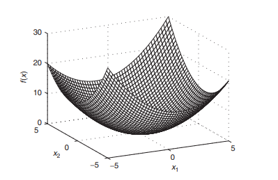
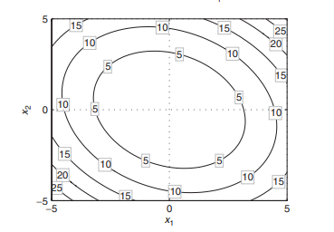
The system of equation $(2.3)$ is often referred to as representing the first-order condition for the objective function extrema. However, it is only a necessary condition; that is, if the gradient is zero at a given point in the $n$-dimensional space, then this point may or may not be a point of a local extremum for the function. An illustration is given in Figure 2.2. The top plot shows the graph of a two-dimensional function and the bottom plot contains the contour lines of the function with the gradient calculated at a grid of points. There are three points marked with a black dot that have a zero gradient. The middle point is not a point of a local maximum even though it has a zero gradient. This point is called a saddle point since the graph resembles the shape of a saddle in a neighborhood of it. The left and the right points are where the function has two local maxima corresponding to the two peaks visible on the top plot. The right peak is a local maximum that is not the global one and the left peak represents the global maximum.
This example demonstrates that the first-order conditions are generally insufficient to characterize the points of local extrema. The additional condition that identifies which of the zero-gradient points are points
of local minimum or maximum is given through the matrix of second derivatives,
$$
H=\left(\begin{array}{cccc}
\frac{\partial^{2} f(x)}{\partial x_{1}^{2}} & \frac{\partial^{2} f(x)}{\partial x_{1} \partial x_{2}} & \cdots & \frac{\partial^{2} f(x)}{\partial x_{1} \partial x_{e}} \
\frac{\partial^{2} f(x)}{\partial x_{2} \partial x_{1}} & \frac{\partial^{2} f(x)}{\partial x_{2}^{2}} & \cdots & \frac{\partial^{2} f(x)}{\partial x_{2} \partial x_{n}} \
\vdots & \vdots & \ddots & \vdots \
\frac{\partial^{2} f(x)}{\partial x_{n} \partial x_{1}} & \frac{\partial^{2} f(x)}{\partial x_{n} \partial x_{2}} & \cdots & \frac{\partial^{2} f(x)}{\partial x_{n}^{2}}
\end{array}\right)
$$
金融代写|风险理论投资组合代写Market Risk, Measures and Portfolio 代考|Convex Functions
In section 2.2.1, we demonstrated that the first-order conditions are insufficient in the general case to describe the local extrema. However, when certain assumptions are made for the objective function, the first-order conditions can become sufficient. Furthermore, for certain classes of functions, the local extrema are necessarily global. Therefore, solving the first-order conditions, we obtain the global extremum.
A general class of functions with nice optimal properties is the class of convex functions. Not only are the convex functions easy to optimize but they have also important application in risk management. In Chapter 6, we discuss general measures of risk. It turns out that the property which guarantees that diversification is possible appears to be exactly the convexity
property. As a consequence, a measure of risk is necessarily a convex functional. ${ }^{1}$
Precisely, a function $f(x)$ is called a convex function if it satisfies the property: For a given $\alpha \in[0,1]$ and all $x^{1} \in \mathbb{R}^{n}$ and $x^{2} \in \mathbb{R}^{n}$ in the function domain,
$$
f\left(\alpha x^{1}+(1-\alpha) x^{2}\right) \leq \alpha f\left(x^{1}\right)+(1-\alpha) f\left(x^{2}\right)
$$
The definition is illustrated in Figure 2.3. Basically, if a function is convex, then a straight line connecting any two points on the graph lies “above” the graph of the function.
There is a related term to convex functions. A function $f$ is called concave if the negative of $f$ is convex. In effect, a function is concave if it
satisfies the property: For a given $\alpha \in[0,1]$ and all $x^{1} \in \mathbb{R}^{n}$ and $x^{2} \in \mathbb{R}^{n}$ in the function domain,
$$
f\left(\alpha x^{1}+(1-\alpha) x^{2}\right) \geq \alpha f\left(x^{1}\right)+(1-\alpha) f\left(x^{2}\right) .
$$
We use convex and concave functions in the discussion of the efficient frontier in Chapter 8 .
If the domain $D$ of a convex function is not the entire space $\mathbb{R}^{n}$, then the set D satisfies the property,
$$
\alpha x^{1}+(1-\alpha) x^{2} \in D
$$
where $x^{1} \in D, x^{2} \in D$, and $0 \leq \alpha \leq 1$. The sets that satisfy equation (2.6) are called convex sets. Thus, the domains of convex (and concave) functions should be convex sets. Geometrically, a set is convex if it contains the straight line connecting any two points belonging to the set. Rockafellar (1997) provides detailed information on the implications of convexity in optimization theory.
We summarize several important properties of convex functions:
- Not all convex functions are differentiable. If a convex function is two times continuously differentiable, then the corresponding Hessian defined in equation $(2.4)$ is a positive semidefinite matrix. ${ }^{2}$
- All convex functions are continuous if considered in an open set.
- The sublevel sets
$$
L_{c}={x: f(x) \leq c}
$$
where $c$ is a constant, are convex sets if $f$ is a convex function. The converse is not true in general. Section $2.2 .3$ provides more information about non-convex functions with convex sublevel sets. - The local minima of a convex function are global. If a convex function $f$ is twice continuously differentiable, then the global minimum is obtained in the points solving the first-order condition,
$$
\nabla f(x)=0 .
$$ - A sum of convex functions is a convex function:
$$
f(x)=f_{1}(x)+f_{2}(x)+\ldots+f_{k}(x)
$$
is a convex function if $f_{i}, i=1, \ldots, k$ are convex functions.
风险理论投资组合代写
金融代写|风险理论投资组合代写Market Risk, Measures and Portfolio 代考|UNCONSTRAINED OPTIMIZATION
当对可行解集没有约束时,我们有一个无约束的优化问题。因此,目标是最大化或最小化关于函数参数的目标函数,而对其值没有任何限制。我们直接考虑n-维案例;即目标函数的域F是个n维空间和函数值是实数,F:Rn→R. 最大化表示为
最大限度F(X1,…,Xn)
和最小化
分钟F(X1,…,Xn)
通常使用更紧凑的形式,例如
分钟X∈RnF(X)表示我们正在寻找函数的最小值F(X)通过改变X在整个n维空间Rn. 方程 (2.1) 的解是X=X0其中最小的F达到,F0=F(X0)=分钟X∈R圆周率F(X).因此,向量X0是这样的,该函数的值大于F0对于任何其他向量X,
F(X0)≤F(X),X∈Rn
请注意,可能有多个向量X0满足等式(2.2)中的不等式,因此,F0实现的可能不是唯一的。如果 (2.2) 成立,则称该函数在X0. 如果不等式在(2.2)为X只属于一个小社区X0而不是整个空间Rn,则称目标函数在X0. 这通常表示为
F(X0)≤F(X)
对全部X这样|X−X0|2<ε在哪里|X−X0|2代表向量之间的欧几里得距离X和X0,
|X−X0|2=∑一世=1n(X一世−X一世0)2
和ε是一些正数。局部最小值可能不是全局的,因为在小邻域之外可能存在向量X0目标函数的值小于F(X0). 数字2.2显示具有两个局部最大值的函数图,其中一个是全局最大值。
最小化和最大化之间存在联系。最大化目标函数与最小化目标函数的负值然后改变最小值的符号相同,
最大限度X∈RnF(X)=−分钟X∈Rn[−F(X)].
这种关系如图 2.1 所示。因此,最大化问题可以用函数最小化来表述,反之亦然。
金融代写|风险理论投资组合代写Market Risk, Measures and Portfolio 代考|Minima and Maxima of a Differentiable Function
如果目标函数的二阶导数存在,则可以表征其局部最大值和最小值,通常称为局部极值。
表示为∇F(X)目标函数的一阶偏导数向量X,
∇F(X)=(∂F(X)∂X1,…,∂F(X)∂Xn).
这个向量称为函数梯度。在每个点X函数的域,它显示了函数在一个小邻域内的最大增长率方向X. 如果对于给定的X,梯度等于一个零向量,
∇F(X)=(0,…,0)
那么函数在X∈Rn. 事实证明,目标函数的所有局部极值点都以零梯度为特征。因此,产生目标函数局部极值的点在方程组的解中,
∣∂F(X)∂X1=0 ⋯ ∂F(X)∂Xn=0
方程组(2.3)通常被称为表示目标函数极值的一阶条件。但是,这只是一个必要条件;也就是说,如果梯度在给定点处为零n维空间,那么这个点可能是也可能不是函数的局部极值点。图 2.2 给出了说明。上图显示了二维函数的图形,下图包含函数的等高线以及在点网格处计算的梯度。三个点用黑点标记,梯度为零。中间点不是局部最大值的点,即使它的梯度为零。这个点被称为鞍点,因为该图类似于它附近的鞍的形状。左点和右点是函数具有两个局部最大值的位置,对应于顶部图上可见的两个峰值。右峰是局部最大值,不是全局最大值,左峰代表全局最大值。
这个例子表明,一阶条件通常不足以表征局部极值点。标识哪些零梯度点是点的附加条件
通过二阶导数矩阵给出局部最小值或最大值,
H=(∂2F(X)∂X12∂2F(X)∂X1∂X2⋯∂2F(X)∂X1∂X和 ∂2F(X)∂X2∂X1∂2F(X)∂X22⋯∂2F(X)∂X2∂Xn ⋮⋮⋱⋮ ∂2F(X)∂Xn∂X1∂2F(X)∂Xn∂X2⋯∂2F(X)∂Xn2)
金融代写|风险理论投资组合代写Market Risk, Measures and Portfolio 代考|Convex Functions
在 2.2.1 节中,我们证明了一阶条件在一般情况下不足以描述局部极值。但是,当对目标函数做出某些假设时,一阶条件可能变得足够。此外,对于某些类别的函数,局部极值必然是全局的。因此,求解一阶条件,我们得到全局极值。
具有良好最优特性的一般函数类是凸函数类。凸函数不仅易于优化,而且在风险管理中也有重要应用。在第 6 章中,我们讨论了风险的一般度量。事实证明,保证多样化是可能的属性似乎正是凸性
财产。因此,风险度量必然是凸泛函。1
准确地说,一个函数F(X)如果满足以下性质,则称为凸函数:对于给定的一种∈[0,1]和所有X1∈Rn和X2∈Rn在功能域中,
F(一种X1+(1−一种)X2)≤一种F(X1)+(1−一种)F(X2)
定义如图 2.3 所示。基本上,如果一个函数是凸函数,那么连接图上任意两点的直线位于函数图的“上方”。
有一个与凸函数相关的术语。一个函数F称为凹的,如果F是凸的。实际上,一个函数是凹的,如果它
满足属性:对于给定的一种∈[0,1]和所有X1∈Rn和X2∈Rn在功能域中,
F(一种X1+(1−一种)X2)≥一种F(X1)+(1−一种)F(X2).
我们在第 8 章讨论有效边界时使用了凸函数和凹函数。
如果域D凸函数的不是整个空间Rn,则集合 D 满足性质,
一种X1+(1−一种)X2∈D
在哪里X1∈D,X2∈D, 和0≤一种≤1. 满足方程(2.6)的集合称为凸集。因此,凸(和凹)函数的域应该是凸集。在几何上,如果一个集合包含连接属于该集合的任意两点的直线,则该集合是凸的。Rockafellar (1997) 提供了关于凸性在优化理论中的含义的详细信息。
我们总结了凸函数的几个重要性质:
- 并非所有凸函数都是可微的。如果一个凸函数是两次连续可微的,则等式中定义的相应 Hessian(2.4)是一个半正定矩阵。2
- 如果在开集中考虑,所有凸函数都是连续的。
- 子级集
大号C=X:F(X)≤C
在哪里C是一个常数,如果是凸集F是一个凸函数。反之亦然。部分2.2.3提供有关具有凸子水平集的非凸函数的更多信息。 - 凸函数的局部最小值是全局的。如果一个凸函数F是两次连续可微的,则在求解一阶条件的点中获得全局最小值,
∇F(X)=0. - 凸函数之和是一个凸函数:
F(X)=F1(X)+F2(X)+…+Fķ(X)
是一个凸函数,如果F一世,一世=1,…,ķ是凸函数。

统计代写请认准statistics-lab™. statistics-lab™为您的留学生涯保驾护航。
金融工程代写
金融工程是使用数学技术来解决金融问题。金融工程使用计算机科学、统计学、经济学和应用数学领域的工具和知识来解决当前的金融问题,以及设计新的和创新的金融产品。
非参数统计代写
非参数统计指的是一种统计方法,其中不假设数据来自于由少数参数决定的规定模型;这种模型的例子包括正态分布模型和线性回归模型。
广义线性模型代考
广义线性模型(GLM)归属统计学领域,是一种应用灵活的线性回归模型。该模型允许因变量的偏差分布有除了正态分布之外的其它分布。
术语 广义线性模型(GLM)通常是指给定连续和/或分类预测因素的连续响应变量的常规线性回归模型。它包括多元线性回归,以及方差分析和方差分析(仅含固定效应)。
有限元方法代写
有限元方法(FEM)是一种流行的方法,用于数值解决工程和数学建模中出现的微分方程。典型的问题领域包括结构分析、传热、流体流动、质量运输和电磁势等传统领域。
有限元是一种通用的数值方法,用于解决两个或三个空间变量的偏微分方程(即一些边界值问题)。为了解决一个问题,有限元将一个大系统细分为更小、更简单的部分,称为有限元。这是通过在空间维度上的特定空间离散化来实现的,它是通过构建对象的网格来实现的:用于求解的数值域,它有有限数量的点。边界值问题的有限元方法表述最终导致一个代数方程组。该方法在域上对未知函数进行逼近。[1] 然后将模拟这些有限元的简单方程组合成一个更大的方程系统,以模拟整个问题。然后,有限元通过变化微积分使相关的误差函数最小化来逼近一个解决方案。
tatistics-lab作为专业的留学生服务机构,多年来已为美国、英国、加拿大、澳洲等留学热门地的学生提供专业的学术服务,包括但不限于Essay代写,Assignment代写,Dissertation代写,Report代写,小组作业代写,Proposal代写,Paper代写,Presentation代写,计算机作业代写,论文修改和润色,网课代做,exam代考等等。写作范围涵盖高中,本科,研究生等海外留学全阶段,辐射金融,经济学,会计学,审计学,管理学等全球99%专业科目。写作团队既有专业英语母语作者,也有海外名校硕博留学生,每位写作老师都拥有过硬的语言能力,专业的学科背景和学术写作经验。我们承诺100%原创,100%专业,100%准时,100%满意。
随机分析代写
随机微积分是数学的一个分支,对随机过程进行操作。它允许为随机过程的积分定义一个关于随机过程的一致的积分理论。这个领域是由日本数学家伊藤清在第二次世界大战期间创建并开始的。
时间序列分析代写
随机过程,是依赖于参数的一组随机变量的全体,参数通常是时间。 随机变量是随机现象的数量表现,其时间序列是一组按照时间发生先后顺序进行排列的数据点序列。通常一组时间序列的时间间隔为一恒定值(如1秒,5分钟,12小时,7天,1年),因此时间序列可以作为离散时间数据进行分析处理。研究时间序列数据的意义在于现实中,往往需要研究某个事物其随时间发展变化的规律。这就需要通过研究该事物过去发展的历史记录,以得到其自身发展的规律。
回归分析代写
多元回归分析渐进(Multiple Regression Analysis Asymptotics)属于计量经济学领域,主要是一种数学上的统计分析方法,可以分析复杂情况下各影响因素的数学关系,在自然科学、社会和经济学等多个领域内应用广泛。
MATLAB代写
MATLAB 是一种用于技术计算的高性能语言。它将计算、可视化和编程集成在一个易于使用的环境中,其中问题和解决方案以熟悉的数学符号表示。典型用途包括:数学和计算算法开发建模、仿真和原型制作数据分析、探索和可视化科学和工程图形应用程序开发,包括图形用户界面构建MATLAB 是一个交互式系统,其基本数据元素是一个不需要维度的数组。这使您可以解决许多技术计算问题,尤其是那些具有矩阵和向量公式的问题,而只需用 C 或 Fortran 等标量非交互式语言编写程序所需的时间的一小部分。MATLAB 名称代表矩阵实验室。MATLAB 最初的编写目的是提供对由 LINPACK 和 EISPACK 项目开发的矩阵软件的轻松访问,这两个项目共同代表了矩阵计算软件的最新技术。MATLAB 经过多年的发展,得到了许多用户的投入。在大学环境中,它是数学、工程和科学入门和高级课程的标准教学工具。在工业领域,MATLAB 是高效研究、开发和分析的首选工具。MATLAB 具有一系列称为工具箱的特定于应用程序的解决方案。对于大多数 MATLAB 用户来说非常重要,工具箱允许您学习和应用专业技术。工具箱是 MATLAB 函数(M 文件)的综合集合,可扩展 MATLAB 环境以解决特定类别的问题。可用工具箱的领域包括信号处理、控制系统、神经网络、模糊逻辑、小波、仿真等。