如果你也在 怎样代写风险理论投资组合这个学科遇到相关的难题，请随时右上角联系我们的24/7代写客服。

为了衡量市场风险，投资者和分析师使用风险值（VaR）方法。风险值建模是一种统计风险管理方法，它可以量化股票或投资组合的潜在损失，以及该潜在损失发生的概率。

statistics-lab™ 为您的留学生涯保驾护航 在代写风险理论投资组合方面已经树立了自己的口碑, 保证靠谱, 高质且原创的统计Statistics代写服务。我们的专家在代写风险理论投资组合代写方面经验极为丰富，各种代写风险理论投资组合相关的作业也就用不着说。

我们提供的风险理论投资组合及其相关学科的代写，服务范围广, 其中包括但不限于:

• Statistical Inference 统计推断
• Statistical Computing 统计计算
• Advanced Probability Theory 高等概率论
• Advanced Mathematical Statistics 高等数理统计学
• (Generalized) Linear Models 广义线性模型
• Statistical Machine Learning 统计机器学习
• Longitudinal Data Analysis 纵向数据分析
• Foundations of Data Science 数据科学基础

金融代写|风险理论投资组合代写Market Risk, Measures and Portfolio 代考|CONSTRAINED OPTIMIZATION

In constructing optimization problems solving practical issues, it is very often the case that certain constraints need to be imposed in order for the optimal solution to make practical sense. For example, long-only portfolio optimization problems require that the portfolio weights, which represent the variables in optimization, should be nonnegative and should sum up to one. According to the notation in this chapter, this corresponds to a problem of the type,
$$
\begin{array}{rl}
\min {x} & f(x) \ \text { subject to } & x^{\prime} e=1 \ & x \geq 0, \end{array} $$ where: $f(x)$ is the objective function. $e \in \mathbb{R}^{n}$ is a vector of ones, $e=(1, \ldots, 1)$. $x^{\prime} e$ equals the sum of all components of $x, x^{\prime} e=\sum{i}^{n} x_{i}$.
$x \geq 0$ means that all components of the vector $x \in \mathbb{R}^{n}$ are nonnegative.
In problem (2.10), we are searching for the minimum of the objective function by varying $x$ only in the set
$$
\mathbf{X}=\left{x \in \mathbb{R}^{n}: \begin{array}{l}
x^{\prime} e=1 \
x \geq 0
\end{array}\right}
$$
which is also called the set of feasible points or the constraint set. A more compact notation, similar to the notation in the unconstrained problems, is sometimes used,
$$
\min _{x \in \mathrm{X}} f(x)
$$
where $\mathbf{X}$ is defined in equation (2.11).
We distinguish between different types of optimization problems depending on the assumed properties for the objective function and the constraint set. If the constraint set contains only equalities, the problem is easier to handle analytically. In this case, the method of Lagrange multipliers is applied. For more general constraint sets, when they are formed

by both equalities and inequalities, the method of Lagrange multipliers is generalized by the Karush-Kuhn-Tucker conditions (KKT conditions). Like the first-order conditions we considered in unconstrained optimization problems, none of the two approaches leads to necessary and sufficient conditions for constrained optimization problems without further assumptions. One of the most general frameworks in which the KKT conditions are necessary and sufficient is that of convex programming. We have a convex programing problem if the objective function is a convex function and the set of feasible points is a convex set. As important subcases of convex optimization, linear programming and convex quadratic programming problems are considered.

In this section, we describe first the method of Lagrange multipliers, which is often applied to special types of mean-variance optimization problems in order to obtain closed-form solutions. Then we proceed with convex programming that is the framework for reward-risk analysis. The mentioned applications of constrained optimization problems is covered in Chapters 8,9 , and 10 .

金融代写|风险理论投资组合代写Market Risk, Measures and Portfolio 代考|Lagrange Multipliers

Consider the following optimization problem in which the set of feasible points is defined by a number of equality constraints,
$$
\begin{array}{rl}
\min {x} & f(x) \ \text { subject to } & b{1}(x)=0 \
& b_{2}(x)=0 \
\cdots \
& b_{k}(x)=0
\end{array}
$$
The functions $h_{i}(x), i=1, \ldots, k$ build up the constraint set. Note that even though the right-hand side of the equality constraints is zero in the classical formulation of the problem given in equation $(2.12)$, this is not restrictive. If in a practical problem the right-hand side happens to be different than zero, it can be equivalently transformed, for example,
$$
\left{x \in \mathbb{R}^{n}: v(x)=c\right} \quad \Longleftrightarrow \quad\left{x \in \mathbb{R}^{n}: h_{1}(x)=v(x)-c=0\right} .
$$
In order to illustrate the necessary condition for optimality valid for (2.12), let us consider the following two-dimensional example:
$$
\begin{aligned}
\min _{x \in \mathbb{R}^{2}} & \frac{1}{2} x^{\prime} C x \
\text { subject to } & x^{\prime} e=1,
\end{aligned}
$$

where the matrix is
$$
C=\left(\begin{array}{cc}
1 & 0.4 \
0.4 & 1
\end{array}\right) .
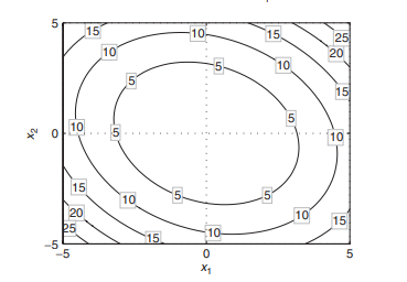
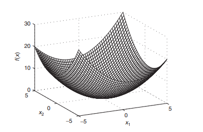
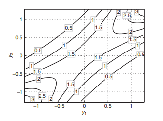
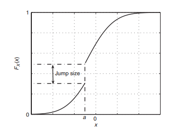
$$
The objective function is a quadratic function and the constraint set contains one linear equality. In Chapter 8, we see that the mean-variance optimization problem in which short positions are allowed is very similar to (2.13). The surface of the objective function and the constraint are shown on the top plot in Figure 2.7. The black line on the surface shows the function values of the feasible points. Geometrically, solving problem (2.13) reduces to finding the lowest point of the black curve on the surface. The contour lines shown on the bottom plot in Figure $2.7$ imply that the feasible point yielding the minimum of the objective function is where a contour line is tangential to the line defined by the equality constraint. On the plot, the tangential contour line and the feasible points are in bold. The black dot indicates the position of the point in which the objective function attains its minimum subject to the constraints.

Even though the example is not general in the sense that the constraint set contains one linear rather than a nonlinear equality, the same geometric intuition applies in the nonlinear case. The fact that the minimum is attained where a contour line is tangential to the curve defined by the nonlinear equality constraints in mathematical language is expressed in the following way: The gradient of the objective function at the point yielding the minimum is proportional to a linear combination of the gradients of the functions defining the constraint set. Formally, this is stated as
$$
\nabla f\left(x^{0}\right)-\mu_{1} \nabla h_{1}\left(x^{0}\right)-\cdots-\mu_{k} \nabla h_{k}\left(x^{0}\right)=0 .
$$
where $\mu_{i}, i=1, \ldots, k$ are some real numbers called Lagrange multipliers and the point $x^{0}$ is such that $f\left(x^{0}\right) \leq f(x)$ for all $x$ that are feasible. Note that if there are no constraints in the problem, then (2.14) reduces to the first-order condition we considered in unconstrained optimization. Therefore, the system of equations behind (2.14) can be viewed as a generalization of the first-order condition in the unconstrained case.

The method of Lagrange multipliers basically associates a function to the problem in $(2.12)$ such that the first-order condition for unconstrained optimization for that function coincides with (2.14). The method of Lagrange multiplier consists of the following steps.

金融代写|风险理论投资组合代写Market Risk, Measures and Portfolio 代考|Convex Programming

The general form of convex programming problems is the following:
$$
\begin{array}{rl}
\min {x} & f(x) \ \text { subject to } & g{i}(x) \leq 0, \quad i=1, \ldots, m \
& h_{j}(x)=0, \quad j=1, \ldots, k,
\end{array}
$$

where:
$f(x)$ is a convex objective function.
$g_{1}(x), \ldots, g_{m}(x)$ are convex functions defining the inequality constraints. $h_{1}(x), \ldots, h_{k}(x)$ are affine functions defining the equality constraints.
Generally, without the assumptions of convexity, problem $(2.17)$ is more involved than $(2.12)$ because besides the equality constraints, there are inequality constraints. The KKT condition, generalizing the method of Lagrange multipliers, is only a necessary condition for optimality in this case. However, adding the assumption of convexity makes the KKT condition necessary and sufficient.

Note that, similar to problem (2.12), the fact that the right-hand side of all constraints is zero is nonrestrictive. The limits can be arbitrary real numbers.
Consider the following two-dimensional optimization problem;
$$
\begin{aligned}
\min {\substack{x \in \mathbb{R}^{2}}} & \frac{1}{2} x^{\prime} \mathrm{C} x \ \text { subject to } &\left(x{1}+2\right)^{2}+\left(x_{2}+2\right)^{2} \leq 3
\end{aligned}
$$
in which
$$
C=\left(\begin{array}{cc}
1 & 0.4 \
0.4 & 1
\end{array}\right) \text {. }
$$
The objective function is a two-dimensional convex quadratic function and the function in the constraint set is also a convex quadratic function. In fact, the boundary of the feasible set is a circle with a radius of $\sqrt{3}$ centered at the point with coordinates $(-2,-2)$. The top plot in Figure $2.8$ shows the surface of the objective function and the set of feasible points. The shaded part on the surface indicates the function values of all feasible points. In fact, solving problem (2.18) reduces to finding the lowest point on the shaded part of the surface. The bottom plot shows the contour lines of the objective function together with the feasible set that is in gray. Geometrically, the point in the feasible set yielding the minimum of the objective function is positioned where a contour line only touches the constraint set. The position of this point is marked with a black dot and the tangential contour line is given in bold.

Note that the solution points of problems of the type $(2.18)$ can happen to be not on the boundary of the feasible set but in the interior. For example, suppose that the radius of the circle defining the boundary of the feasible set in $(2.18)$ is a larger number such that the point $(0,0)$ is inside the feasible

set. Then, the point $(0,0)$ is the solution to problem $(2.18)$ because at this point the objective function attains its global minimum.

In the two-dimensional case, when we can visualize the optimization problem, geometric reasoning guides us to finding the optimal solution point. In a higher dimensional space, plots cannot be produced and we rely on the analytic method behind the KKT conditions.

风险理论投资组合代写

金融代写|风险理论投资组合代写Market Risk, Measures and Portfolio 代考|CONSTRAINED OPTIMIZATION

在构建解决实际问题的优化问题时，通常需要施加某些约束以使最优解具有实际意义。例如，只做多的投资组合优化问题要求代表优化中变量的投资组合权重应该是非负的，并且应该总和为 1。根据本章中的符号，这对应于类型的问题，
分钟XF(X)  受制于 X′和=1 X≥0,在哪里：F(X)是目标函数。和∈Rn是一个向量，和=(1,…,1). X′和等于所有组件的总和X,X′和=∑一世nX一世.
X≥0表示向量的所有分量X∈Rn是非负的。
在问题 (2.10) 中，我们通过改变来寻找目标函数的最小值X仅在集合中
\mathbf{X}=\left{x \in \mathbb{R}^{n}: \begin{array}{l} x^{\prime} e=1 \ x \geq 0 \end{array}\对}\mathbf{X}=\left{x \in \mathbb{R}^{n}: \begin{array}{l} x^{\prime} e=1 \ x \geq 0 \end{array}\对}
也称为可行点集或约束集。有时会使用更紧凑的符号，类似于无约束问题中的符号，
分钟X∈XF(X)
在哪里X在方程（2.11）中定义。
我们根据目标函数和约束集的假设属性来区分不同类型的优化问题。如果约束集仅包含等式，则问题更易于分析处理。在这种情况下，应用拉格朗日乘子法。对于更一般的约束集，当它们形成时

通过等式和不等式，拉格朗日乘子法由 Karush-Kuhn-Tucker 条件（KKT 条件）推广。就像我们在无约束优化问题中考虑的一阶条件一样，如果没有进一步的假设，这两种方法都不会导致约束优化问题的充分必要条件。KKT 条件是必要和充分的最一般框架之一是凸规划。如果目标函数是一个凸函数并且可行点集是一个凸集，那么我们就有一个凸规划问题。作为凸优化的重要子案例，考虑了线性规划和凸二次规划问题。

在本节中，我们首先描述拉格朗日乘子方法，该方法通常应用于特殊类型的均值方差优化问题以获得封闭形式的解。然后我们继续进行凸规划，这是奖励风险分析的框架。第 8、9 和 10 章介绍了约束优化问题的上述应用。

金融代写|风险理论投资组合代写Market Risk, Measures and Portfolio 代考|Lagrange Multipliers

考虑以下优化问题，其中可行点集由多个等式约束定义，
分钟XF(X)  受制于 b1(X)=0 b2(X)=0 ⋯ bķ(X)=0
功能H一世(X),一世=1,…,ķ建立约束集。请注意，即使等式约束的右侧在方程中给出的问题的经典公式中为零(2.12), 这不是限制性的。如果在实际问题中右侧恰好不为零，则可以对其进行等价变换，例如，
\left{x \in \mathbb{R}^{n}: v(x)=c\right} \quad \Longleftrightarrow \quad\left{x \in \mathbb{R}^{n}: h_{1 }(x)=v(x)-c=0\right} 。\left{x \in \mathbb{R}^{n}: v(x)=c\right} \quad \Longleftrightarrow \quad\left{x \in \mathbb{R}^{n}: h_{1 }(x)=v(x)-c=0\right} 。
为了说明对 (2.12) 有效的最优性的必要条件，让我们考虑以下二维示例：
分钟X∈R212X′CX  受制于 X′和=1,

矩阵在哪里
C=(10.4 0.41).
目标函数是二次函数，约束集包含一个线性等式。在第 8 章中，我们看到允许空头头寸的均值方差优化问题与（2.13）非常相似。目标函数的表面和约束显示在图 2.7 的顶部图上。表面上的黑线表示可行点的函数值。在几何上，解决问题 (2.13) 简化为找到曲面上黑色曲线的最低点。图中底部图上显示的等高线2.7暗示产生目标函数最小值的可行点是轮廓线与由等式约束定义的线相切的地方。在图上，切线等高线和可行点以粗体显示。黑点表示目标函数在约束条件下达到其最小值的点的位置。

尽管该示例在约束集包含一个线性而不是非线性等式的意义上不是一般的，但相同的几何直觉适用于非线性情况。在等高线与由数学语言中的非线性等式约束定义的曲线相切时，达到最小值的事实用以下方式表示： 目标函数在产生最小值的点处的梯度与线性组合成比例定义约束集的函数的梯度。正式地，这被表述为
∇F(X0)−μ1∇H1(X0)−⋯−μķ∇Hķ(X0)=0.
在哪里μ一世,一世=1,…,ķ是一些实数，称为拉格朗日乘数和点X0是这样的F(X0)≤F(X)对全部X这是可行的。请注意，如果问题中没有约束，则 (2.14) 简化为我们在无约束优化中考虑的一阶条件。因此，(2.14) 后面的方程组可以看作是无约束情况下一阶条件的推广。

拉格朗日乘子法基本上将函数与问题相关联(2.12)使得该函数的无约束优化的一阶条件与 (2.14) 一致。拉格朗日乘子法由以下步骤组成。

金融代写|风险理论投资组合代写Market Risk, Measures and Portfolio 代考|Convex Programming

凸规划问题的一般形式如下：
分钟XF(X)  受制于 G一世(X)≤0,一世=1,…,米 Hj(X)=0,j=1,…,ķ,

在哪里：
F(X)是一个凸目标函数。
G1(X),…,G米(X)是定义不等式约束的凸函数。H1(X),…,Hķ(X)是定义等式约束的仿射函数。
一般来说，在没有凸性假设的情况下，问题(2.17)比(2.12)因为除了等式约束，还有不等式约束。KKT 条件是拉格朗日乘子法的推广，在这种情况下只是最优性的必要条件。然而，添加凸性假设使得 KKT 条件是必要且充分的。

请注意，与问题 (2.12) 类似，所有约束的右侧为零的事实是非限制性的。限制可以是任意实数。
考虑以下二维优化问题；
分钟X∈R212X′CX  受制于 (X1+2)2+(X2+2)2≤3
其中
C=(10.4 0.41). 
目标函数是一个二维凸二次函数，约束集中的函数也是一个凸二次函数。实际上，可行集的边界是一个半径为3以坐标点为中心(−2,−2). 图中的顶部图2.8显示了目标函数的曲面和可行点集。表面阴影部分表示所有可行点的函数值。事实上，解决问题 (2.18) 可以简化为在曲面的阴影部分找到最低点。底部图显示了目标函数的等高线以及灰色的可行集。在几何上，可行集中产生目标函数最小值的点位于轮廓线仅接触约束集的位置。该点的位置用黑点标记，切线轮廓线用粗体表示。

注意类型问题的解点(2.18)可能恰好不在可行集的边界上，而是在内部。例如，假设定义可行集边界的圆的半径为(2.18)是一个更大的数，使得该点(0,0)在可行范围内

放。那么，重点(0,0)是解决问题的方法(2.18)因为此时目标函数达到其全局最小值。

在二维情况下，当我们可以可视化优化问题时，几何推理会引导我们找到最优解点。在更高维度的空间中，无法生成图，我们依赖于 KKT 条件背后的分析方法。

统计代写请认准statistics-lab™. statistics-lab™为您的留学生涯保驾护航。

金融工程代写

金融工程是使用数学技术来解决金融问题。金融工程使用计算机科学、统计学、经济学和应用数学领域的工具和知识来解决当前的金融问题，以及设计新的和创新的金融产品。

非参数统计代写

非参数统计指的是一种统计方法，其中不假设数据来自于由少数参数决定的规定模型；这种模型的例子包括正态分布模型和线性回归模型。

广义线性模型代考

广义线性模型（GLM）归属统计学领域，是一种应用灵活的线性回归模型。该模型允许因变量的偏差分布有除了正态分布之外的其它分布。

术语 广义线性模型（GLM）通常是指给定连续和/或分类预测因素的连续响应变量的常规线性回归模型。它包括多元线性回归，以及方差分析和方差分析（仅含固定效应）。

有限元方法代写

有限元方法（FEM）是一种流行的方法，用于数值解决工程和数学建模中出现的微分方程。典型的问题领域包括结构分析、传热、流体流动、质量运输和电磁势等传统领域。

有限元是一种通用的数值方法，用于解决两个或三个空间变量的偏微分方程（即一些边界值问题）。为了解决一个问题，有限元将一个大系统细分为更小、更简单的部分，称为有限元。这是通过在空间维度上的特定空间离散化来实现的，它是通过构建对象的网格来实现的：用于求解的数值域，它有有限数量的点。边界值问题的有限元方法表述最终导致一个代数方程组。该方法在域上对未知函数进行逼近。[1] 然后将模拟这些有限元的简单方程组合成一个更大的方程系统，以模拟整个问题。然后，有限元通过变化微积分使相关的误差函数最小化来逼近一个解决方案。

tatistics-lab作为专业的留学生服务机构，多年来已为美国、英国、加拿大、澳洲等留学热门地的学生提供专业的学术服务，包括但不限于Essay代写，Assignment代写，Dissertation代写，Report代写，小组作业代写，Proposal代写，Paper代写，Presentation代写，计算机作业代写，论文修改和润色，网课代做，exam代考等等。写作范围涵盖高中，本科，研究生等海外留学全阶段，辐射金融，经济学，会计学，审计学，管理学等全球99%专业科目。写作团队既有专业英语母语作者，也有海外名校硕博留学生，每位写作老师都拥有过硬的语言能力，专业的学科背景和学术写作经验。我们承诺100%原创，100%专业，100%准时，100%满意。

随机分析代写

随机微积分是数学的一个分支，对随机过程进行操作。它允许为随机过程的积分定义一个关于随机过程的一致的积分理论。这个领域是由日本数学家伊藤清在第二次世界大战期间创建并开始的。

时间序列分析代写

随机过程，是依赖于参数的一组随机变量的全体，参数通常是时间。 随机变量是随机现象的数量表现，其时间序列是一组按照时间发生先后顺序进行排列的数据点序列。通常一组时间序列的时间间隔为一恒定值（如1秒，5分钟，12小时，7天，1年），因此时间序列可以作为离散时间数据进行分析处理。研究时间序列数据的意义在于现实中，往往需要研究某个事物其随时间发展变化的规律。这就需要通过研究该事物过去发展的历史记录，以得到其自身发展的规律。

回归分析代写

多元回归分析渐进（Multiple Regression Analysis Asymptotics）属于计量经济学领域，主要是一种数学上的统计分析方法，可以分析复杂情况下各影响因素的数学关系，在自然科学、社会和经济学等多个领域内应用广泛。

MATLAB代写

MATLAB 是一种用于技术计算的高性能语言。它将计算、可视化和编程集成在一个易于使用的环境中，其中问题和解决方案以熟悉的数学符号表示。典型用途包括：数学和计算算法开发建模、仿真和原型制作数据分析、探索和可视化科学和工程图形应用程序开发，包括图形用户界面构建MATLAB 是一个交互式系统，其基本数据元素是一个不需要维度的数组。这使您可以解决许多技术计算问题，尤其是那些具有矩阵和向量公式的问题，而只需用 C 或 Fortran 等标量非交互式语言编写程序所需的时间的一小部分。MATLAB 名称代表矩阵实验室。MATLAB 最初的编写目的是提供对由 LINPACK 和 EISPACK 项目开发的矩阵软件的轻松访问，这两个项目共同代表了矩阵计算软件的最新技术。MATLAB 经过多年的发展，得到了许多用户的投入。在大学环境中，它是数学、工程和科学入门和高级课程的标准教学工具。在工业领域，MATLAB 是高效研究、开发和分析的首选工具。MATLAB 具有一系列称为工具箱的特定于应用程序的解决方案。对于大多数 MATLAB 用户来说非常重要，工具箱允许您学习和应用专业技术。工具箱是 MATLAB 函数（M 文件）的综合集合，可扩展 MATLAB 环境以解决特定类别的问题。可用工具箱的领域包括信号处理、控制系统、神经网络、模糊逻辑、小波、仿真等。

R语言代写	问卷设计与分析代写
PYTHON代写	回归分析与线性模型代写
MATLAB代写	方差分析与试验设计代写
STATA代写	机器学习/统计学习代写
SPSS代写	计量经济学代写
EVIEWS代写	时间序列分析代写
EXCEL代写	深度学习代写
SQL代写	各种数据建模与可视化代写

如果你也在 怎样代写风险理论投资组合这个学科遇到相关的难题，请随时右上角联系我们的24/7代写客服。

为了衡量市场风险，投资者和分析师使用风险值（VaR）方法。风险值建模是一种统计风险管理方法，它可以量化股票或投资组合的潜在损失，以及该潜在损失发生的概率。

statistics-lab™ 为您的留学生涯保驾护航 在代写风险理论投资组合方面已经树立了自己的口碑, 保证靠谱, 高质且原创的统计Statistics代写服务。我们的专家在代写风险理论投资组合代写方面经验极为丰富，各种代写风险理论投资组合相关的作业也就用不着说。

我们提供的风险理论投资组合及其相关学科的代写，服务范围广, 其中包括但不限于:

• Statistical Inference 统计推断
• Statistical Computing 统计计算
• Advanced Probability Theory 高等概率论
• Advanced Mathematical Statistics 高等数理统计学
• (Generalized) Linear Models 广义线性模型
• Statistical Machine Learning 统计机器学习
• Longitudinal Data Analysis 纵向数据分析
• Foundations of Data Science 数据科学基础

金融代写|风险理论投资组合代写Market Risk, Measures and Portfolio 代考|UNCONSTRAINED OPTIMIZATION

When there are no constraints imposed on the set of feasible solutions, we have an unconstrained optimization problem. Thus, the goal is to maximize or to minimize the objective function with respect to the function arguments without any limits on their values. We consider directly the $n$-dimensional case; that is, the domain of the objective function $f$ is the $n$-dimensional space and the function values are real numbers, $f: \mathbb{R}^{n} \rightarrow \mathbb{R}$. Maximization is denoted by
$$
\max f\left(x_{1}, \ldots, x_{n}\right)
$$
and minimization by
$$
\min f\left(x_{1}, \ldots, x_{n}\right)
$$
A more compact form is commonly used, for example
$$
\min {x \in \mathbb{R}^{n}} f(x) $$ denotes that we are searching for the minimal value of the function $f(x)$ by varying $x$ in the entire $n$-dimensional space $\mathbb{R}^{n}$. A solution to equation (2.1) is a value of $x=x^{0}$ for which the minimum of $f$ is attained, $$ f{0}=f\left(x^{0}\right)=\min {x \in \mathbb{R}^{\pi}} f(x) . $$ Thus, the vector $x{0}$ is such that the function takes a larger value than $f_{0}$ for any other vector $x$,
$$
f\left(x^{0}\right) \leq f(x), x \in \mathbb{R}^{n}
$$
Note that there may be more than one vector $x^{0}$ satisfying the inequality in equation (2.2) and, therefore, the argument for which $f_{0}$ is achieved may not be unique. If (2.2) holds, then the function is said to attain its global minimum at $x^{0}$. If the inequality in $(2.2)$ holds for $x$ belonging only to a small neighborhood of $x^{0}$ and not to the entire space $\mathbb{R}^{n}$, then the objective function is said to have a local minimum at $x^{0}$. This is usually denoted by
$$
f\left(x^{0}\right) \leq f(x)
$$

for all $x$ such that $\left|x-x^{0}\right|_{2}<\epsilon$ where $\left|x-x^{0}\right|_{2}$ stands for the Euclidean distance between the vectors $x$ and $x^{0}$,
$$
\left|x-x^{0}\right|_{2}=\sqrt{\sum_{i=1}^{n}\left(x_{i}-x_{i}^{0}\right)^{2}}
$$
and $\epsilon$ is some positive number. A local minimum may not be global as there may be vectors outside the small neighborhood of $x_{0}$ for which the objective function attains a smaller value than $f\left(x_{0}\right)$. Figure $2.2$ shows the graph of a function with two local maxima, one of which is the global maximum.

There is a connection between minimization and maximization. Maximizing the objective function is the same as minimizing the negative of the objective function and then changing the sign of the minimal value,
$$
\max {x \in \mathbb{R}^{n}} f(x)=-\min {x \in \mathbb{R}^{n}}[-f(x)] .
$$
This relationship is illustrated in Figure 2.1. As a consequence, problems for maximization can be stated in terms of function minimization and vice versa.

金融代写|风险理论投资组合代写Market Risk, Measures and Portfolio 代考|Minima and Maxima of a Differentiable Function

If the second derivatives of the objective function exist, then its local maxima and minima, often called generically local extrema, can be characterized.

Denote by $\nabla f(x)$ the vector of the first partial derivatives of the objective function evaluated at $x$,
$$
\nabla f(x)=\left(\frac{\partial f(x)}{\partial x_{1}}, \ldots, \frac{\partial f(x)}{\partial x_{n}}\right) .
$$
This vector is called the function gradient. At each point $x$ of the domain of the function, it shows the direction of greatest rate of increase of the function in a small neighborhood of $x$. If for a given $x$, the gradient equals a vector of zeros,
$$
\nabla f(x)=(0, \ldots, 0)
$$
then the function does not change in a small neighborhood of $x \in \mathbb{R}^{n}$. It turns out that all points of local extrema of the objective function are characterized by a zero gradient. As a result, the points yielding the local extrema of the objective function are among the solutions of the system of equations,
$$
\mid \begin{aligned}
&\frac{\partial f(x)}{\partial x_{1}}=0 \
&\cdots \
&\frac{\partial f(x)}{\partial x_{n}}=0
\end{aligned}
$$
The system of equation $(2.3)$ is often referred to as representing the first-order condition for the objective function extrema. However, it is only a necessary condition; that is, if the gradient is zero at a given point in the $n$-dimensional space, then this point may or may not be a point of a local extremum for the function. An illustration is given in Figure 2.2. The top plot shows the graph of a two-dimensional function and the bottom plot contains the contour lines of the function with the gradient calculated at a grid of points. There are three points marked with a black dot that have a zero gradient. The middle point is not a point of a local maximum even though it has a zero gradient. This point is called a saddle point since the graph resembles the shape of a saddle in a neighborhood of it. The left and the right points are where the function has two local maxima corresponding to the two peaks visible on the top plot. The right peak is a local maximum that is not the global one and the left peak represents the global maximum.

This example demonstrates that the first-order conditions are generally insufficient to characterize the points of local extrema. The additional condition that identifies which of the zero-gradient points are points

of local minimum or maximum is given through the matrix of second derivatives,
$$
H=\left(\begin{array}{cccc}
\frac{\partial^{2} f(x)}{\partial x_{1}^{2}} & \frac{\partial^{2} f(x)}{\partial x_{1} \partial x_{2}} & \cdots & \frac{\partial^{2} f(x)}{\partial x_{1} \partial x_{e}} \
\frac{\partial^{2} f(x)}{\partial x_{2} \partial x_{1}} & \frac{\partial^{2} f(x)}{\partial x_{2}^{2}} & \cdots & \frac{\partial^{2} f(x)}{\partial x_{2} \partial x_{n}} \
\vdots & \vdots & \ddots & \vdots \
\frac{\partial^{2} f(x)}{\partial x_{n} \partial x_{1}} & \frac{\partial^{2} f(x)}{\partial x_{n} \partial x_{2}} & \cdots & \frac{\partial^{2} f(x)}{\partial x_{n}^{2}}
\end{array}\right)
$$

金融代写|风险理论投资组合代写Market Risk, Measures and Portfolio 代考|Convex Functions

In section 2.2.1, we demonstrated that the first-order conditions are insufficient in the general case to describe the local extrema. However, when certain assumptions are made for the objective function, the first-order conditions can become sufficient. Furthermore, for certain classes of functions, the local extrema are necessarily global. Therefore, solving the first-order conditions, we obtain the global extremum.

A general class of functions with nice optimal properties is the class of convex functions. Not only are the convex functions easy to optimize but they have also important application in risk management. In Chapter 6, we discuss general measures of risk. It turns out that the property which guarantees that diversification is possible appears to be exactly the convexity

property. As a consequence, a measure of risk is necessarily a convex functional. ${ }^{1}$

Precisely, a function $f(x)$ is called a convex function if it satisfies the property: For a given $\alpha \in[0,1]$ and all $x^{1} \in \mathbb{R}^{n}$ and $x^{2} \in \mathbb{R}^{n}$ in the function domain,
$$
f\left(\alpha x^{1}+(1-\alpha) x^{2}\right) \leq \alpha f\left(x^{1}\right)+(1-\alpha) f\left(x^{2}\right)
$$
The definition is illustrated in Figure 2.3. Basically, if a function is convex, then a straight line connecting any two points on the graph lies “above” the graph of the function.

There is a related term to convex functions. A function $f$ is called concave if the negative of $f$ is convex. In effect, a function is concave if it

satisfies the property: For a given $\alpha \in[0,1]$ and all $x^{1} \in \mathbb{R}^{n}$ and $x^{2} \in \mathbb{R}^{n}$ in the function domain,
$$
f\left(\alpha x^{1}+(1-\alpha) x^{2}\right) \geq \alpha f\left(x^{1}\right)+(1-\alpha) f\left(x^{2}\right) .
$$
We use convex and concave functions in the discussion of the efficient frontier in Chapter 8 .

If the domain $D$ of a convex function is not the entire space $\mathbb{R}^{n}$, then the set D satisfies the property,
$$
\alpha x^{1}+(1-\alpha) x^{2} \in D
$$
where $x^{1} \in D, x^{2} \in D$, and $0 \leq \alpha \leq 1$. The sets that satisfy equation (2.6) are called convex sets. Thus, the domains of convex (and concave) functions should be convex sets. Geometrically, a set is convex if it contains the straight line connecting any two points belonging to the set. Rockafellar (1997) provides detailed information on the implications of convexity in optimization theory.
We summarize several important properties of convex functions:

• Not all convex functions are differentiable. If a convex function is two times continuously differentiable, then the corresponding Hessian defined in equation $(2.4)$ is a positive semidefinite matrix. ${ }^{2}$
• All convex functions are continuous if considered in an open set.
• The sublevel sets
  $$
  L_{c}={x: f(x) \leq c}
  $$
  where $c$ is a constant, are convex sets if $f$ is a convex function. The converse is not true in general. Section $2.2 .3$ provides more information about non-convex functions with convex sublevel sets.
• The local minima of a convex function are global. If a convex function $f$ is twice continuously differentiable, then the global minimum is obtained in the points solving the first-order condition,
  $$
  \nabla f(x)=0 .
  $$
• A sum of convex functions is a convex function:
  $$
  f(x)=f_{1}(x)+f_{2}(x)+\ldots+f_{k}(x)
  $$
  is a convex function if $f_{i}, i=1, \ldots, k$ are convex functions.

风险理论投资组合代写

金融代写|风险理论投资组合代写Market Risk, Measures and Portfolio 代考|UNCONSTRAINED OPTIMIZATION

当对可行解集没有约束时，我们有一个无约束的优化问题。因此，目标是最大化或最小化关于函数参数的目标函数，而对其值没有任何限制。我们直接考虑n-维案例；即目标函数的域F是个n维空间和函数值是实数，F:Rn→R. 最大化表示为
最大限度F(X1,…,Xn)
和最小化
分钟F(X1,…,Xn)
通常使用更紧凑的形式，例如
分钟X∈RnF(X)表示我们正在寻找函数的最小值F(X)通过改变X在整个n维空间Rn. 方程 (2.1) 的解是X=X0其中最小的F达到，F0=F(X0)=分钟X∈R圆周率F(X).因此，向量X0是这样的，该函数的值大于F0对于任何其他向量X,
F(X0)≤F(X),X∈Rn
请注意，可能有多个向量X0满足等式（2.2）中的不等式，因此，F0实现的可能不是唯一的。如果 (2.2) 成立，则称该函数在X0. 如果不等式在(2.2)为X只属于一个小社区X0而不是整个空间Rn，则称目标函数在X0. 这通常表示为
F(X0)≤F(X)

对全部X这样|X−X0|2<ε在哪里|X−X0|2代表向量之间的欧几里得距离X和X0,
|X−X0|2=∑一世=1n(X一世−X一世0)2
和ε是一些正数。局部最小值可能不是全局的，因为在小邻域之外可能存在向量X0目标函数的值小于F(X0). 数字2.2显示具有两个局部最大值的函数图，其中一个是全局最大值。

最小化和最大化之间存在联系。最大化目标函数与最小化目标函数的负值然后改变最小值的符号相同，
最大限度X∈RnF(X)=−分钟X∈Rn[−F(X)].
这种关系如图 2.1 所示。因此，最大化问题可以用函数最小化来表述，反之亦然。

金融代写|风险理论投资组合代写Market Risk, Measures and Portfolio 代考|Minima and Maxima of a Differentiable Function

如果目标函数的二阶导数存在，则可以表征其局部最大值和最小值，通常称为局部极值。

表示为∇F(X)目标函数的一阶偏导数向量X,
∇F(X)=(∂F(X)∂X1,…,∂F(X)∂Xn).
这个向量称为函数梯度。在每个点X函数的域，它显示了函数在一个小邻域内的最大增长率方向X. 如果对于给定的X，梯度等于一个零向量，
∇F(X)=(0,…,0)
那么函数在X∈Rn. 事实证明，目标函数的所有局部极值点都以零梯度为特征。因此，产生目标函数局部极值的点在方程组的解中，
∣∂F(X)∂X1=0 ⋯ ∂F(X)∂Xn=0
方程组(2.3)通常被称为表示目标函数极值的一阶条件。但是，这只是一个必要条件；也就是说，如果梯度在给定点处为零n维空间，那么这个点可能是也可能不是函数的局部极值点。图 2.2 给出了说明。上图显示了二维函数的图形，下图包含函数的等高线以及在点网格处计算的梯度。三个点用黑点标记，梯度为零。中间点不是局部最大值的点，即使它的梯度为零。这个点被称为鞍点，因为该图类似于它附近的鞍的形状。左点和右点是函数具有两个局部最大值的位置，对应于顶部图上可见的两个峰值。右峰是局部最大值，不是全局最大值，左峰代表全局最大值。

这个例子表明，一阶条件通常不足以表征局部极值点。标识哪些零梯度点是点的附加条件

通过二阶导数矩阵给出局部最小值或最大值，
H=(∂2F(X)∂X12∂2F(X)∂X1∂X2⋯∂2F(X)∂X1∂X和 ∂2F(X)∂X2∂X1∂2F(X)∂X22⋯∂2F(X)∂X2∂Xn ⋮⋮⋱⋮ ∂2F(X)∂Xn∂X1∂2F(X)∂Xn∂X2⋯∂2F(X)∂Xn2)

金融代写|风险理论投资组合代写Market Risk, Measures and Portfolio 代考|Convex Functions

在 2.2.1 节中，我们证明了一阶条件在一般情况下不足以描述局部极值。但是，当对目标函数做出某些假设时，一阶条件可能变得足够。此外，对于某些类别的函数，局部极值必然是全局的。因此，求解一阶条件，我们得到全局极值。

具有良好最优特性的一般函数类是凸函数类。凸函数不仅易于优化，而且在风险管理中也有重要应用。在第 6 章中，我们讨论了风险的一般度量。事实证明，保证多样化是可能的属性似乎正是凸性

财产。因此，风险度量必然是凸泛函。1

准确地说，一个函数F(X)如果满足以下性质，则称为凸函数：对于给定的一种∈[0,1]和所有X1∈Rn和X2∈Rn在功能域中，
F(一种X1+(1−一种)X2)≤一种F(X1)+(1−一种)F(X2)
定义如图 2.3 所示。基本上，如果一个函数是凸函数，那么连接图上任意两点的直线位于函数图的“上方”。

有一个与凸函数相关的术语。一个函数F称为凹的，如果F是凸的。实际上，一个函数是凹的，如果它

满足属性：对于给定的一种∈[0,1]和所有X1∈Rn和X2∈Rn在功能域中，
F(一种X1+(1−一种)X2)≥一种F(X1)+(1−一种)F(X2).
我们在第 8 章讨论有效边界时使用了凸函数和凹函数。

如果域D凸函数的不是整个空间Rn，则集合 D 满足性质，
一种X1+(1−一种)X2∈D
在哪里X1∈D,X2∈D， 和0≤一种≤1. 满足方程（2.6）的集合称为凸集。因此，凸（和凹）函数的域应该是凸集。在几何上，如果一个集合包含连接属于该集合的任意两点的直线，则该集合是凸的。Rockafellar (1997) 提供了关于凸性在优化理论中的含义的详细信息。
我们总结了凸函数的几个重要性质：

• 并非所有凸函数都是可微的。如果一个凸函数是两次连续可微的，则等式中定义的相应 Hessian(2.4)是一个半正定矩阵。2
• 如果在开集中考虑，所有凸函数都是连续的。
• 子级集
  大号C=X:F(X)≤C
  在哪里C是一个常数，如果是凸集F是一个凸函数。反之亦然。部分2.2.3提供有关具有凸子水平集的非凸函数的更多信息。
• 凸函数的局部最小值是全局的。如果一个凸函数F是两次连续可微的，则在求解一阶条件的点中获得全局最小值，
  ∇F(X)=0.
• 凸函数之和是一个凸函数：
  F(X)=F1(X)+F2(X)+…+Fķ(X)
  是一个凸函数，如果F一世,一世=1,…,ķ是凸函数。

统计代写请认准statistics-lab™. statistics-lab™为您的留学生涯保驾护航。

金融工程代写

金融工程是使用数学技术来解决金融问题。金融工程使用计算机科学、统计学、经济学和应用数学领域的工具和知识来解决当前的金融问题，以及设计新的和创新的金融产品。

非参数统计代写

非参数统计指的是一种统计方法，其中不假设数据来自于由少数参数决定的规定模型；这种模型的例子包括正态分布模型和线性回归模型。

广义线性模型代考

广义线性模型（GLM）归属统计学领域，是一种应用灵活的线性回归模型。该模型允许因变量的偏差分布有除了正态分布之外的其它分布。

术语 广义线性模型（GLM）通常是指给定连续和/或分类预测因素的连续响应变量的常规线性回归模型。它包括多元线性回归，以及方差分析和方差分析（仅含固定效应）。

有限元方法代写

有限元方法（FEM）是一种流行的方法，用于数值解决工程和数学建模中出现的微分方程。典型的问题领域包括结构分析、传热、流体流动、质量运输和电磁势等传统领域。

有限元是一种通用的数值方法，用于解决两个或三个空间变量的偏微分方程（即一些边界值问题）。为了解决一个问题，有限元将一个大系统细分为更小、更简单的部分，称为有限元。这是通过在空间维度上的特定空间离散化来实现的，它是通过构建对象的网格来实现的：用于求解的数值域，它有有限数量的点。边界值问题的有限元方法表述最终导致一个代数方程组。该方法在域上对未知函数进行逼近。[1] 然后将模拟这些有限元的简单方程组合成一个更大的方程系统，以模拟整个问题。然后，有限元通过变化微积分使相关的误差函数最小化来逼近一个解决方案。

tatistics-lab作为专业的留学生服务机构，多年来已为美国、英国、加拿大、澳洲等留学热门地的学生提供专业的学术服务，包括但不限于Essay代写，Assignment代写，Dissertation代写，Report代写，小组作业代写，Proposal代写，Paper代写，Presentation代写，计算机作业代写，论文修改和润色，网课代做，exam代考等等。写作范围涵盖高中，本科，研究生等海外留学全阶段，辐射金融，经济学，会计学，审计学，管理学等全球99%专业科目。写作团队既有专业英语母语作者，也有海外名校硕博留学生，每位写作老师都拥有过硬的语言能力，专业的学科背景和学术写作经验。我们承诺100%原创，100%专业，100%准时，100%满意。

随机分析代写

随机微积分是数学的一个分支，对随机过程进行操作。它允许为随机过程的积分定义一个关于随机过程的一致的积分理论。这个领域是由日本数学家伊藤清在第二次世界大战期间创建并开始的。

时间序列分析代写

随机过程，是依赖于参数的一组随机变量的全体，参数通常是时间。 随机变量是随机现象的数量表现，其时间序列是一组按照时间发生先后顺序进行排列的数据点序列。通常一组时间序列的时间间隔为一恒定值（如1秒，5分钟，12小时，7天，1年），因此时间序列可以作为离散时间数据进行分析处理。研究时间序列数据的意义在于现实中，往往需要研究某个事物其随时间发展变化的规律。这就需要通过研究该事物过去发展的历史记录，以得到其自身发展的规律。

回归分析代写

多元回归分析渐进（Multiple Regression Analysis Asymptotics）属于计量经济学领域，主要是一种数学上的统计分析方法，可以分析复杂情况下各影响因素的数学关系，在自然科学、社会和经济学等多个领域内应用广泛。

MATLAB代写

MATLAB 是一种用于技术计算的高性能语言。它将计算、可视化和编程集成在一个易于使用的环境中，其中问题和解决方案以熟悉的数学符号表示。典型用途包括：数学和计算算法开发建模、仿真和原型制作数据分析、探索和可视化科学和工程图形应用程序开发，包括图形用户界面构建MATLAB 是一个交互式系统，其基本数据元素是一个不需要维度的数组。这使您可以解决许多技术计算问题，尤其是那些具有矩阵和向量公式的问题，而只需用 C 或 Fortran 等标量非交互式语言编写程序所需的时间的一小部分。MATLAB 名称代表矩阵实验室。MATLAB 最初的编写目的是提供对由 LINPACK 和 EISPACK 项目开发的矩阵软件的轻松访问，这两个项目共同代表了矩阵计算软件的最新技术。MATLAB 经过多年的发展，得到了许多用户的投入。在大学环境中，它是数学、工程和科学入门和高级课程的标准教学工具。在工业领域，MATLAB 是高效研究、开发和分析的首选工具。MATLAB 具有一系列称为工具箱的特定于应用程序的解决方案。对于大多数 MATLAB 用户来说非常重要，工具箱允许您学习和应用专业技术。工具箱是 MATLAB 函数（M 文件）的综合集合，可扩展 MATLAB 环境以解决特定类别的问题。可用工具箱的领域包括信号处理、控制系统、神经网络、模糊逻辑、小波、仿真等。

R语言代写	问卷设计与分析代写
PYTHON代写	回归分析与线性模型代写
MATLAB代写	方差分析与试验设计代写
STATA代写	机器学习/统计学习代写
SPSS代写	计量经济学代写
EVIEWS代写	时间序列分析代写
EXCEL代写	深度学习代写
SQL代写	各种数据建模与可视化代写

如果你也在 怎样代写风险理论投资组合这个学科遇到相关的难题，请随时右上角联系我们的24/7代写客服。

为了衡量市场风险，投资者和分析师使用风险值（VaR）方法。风险值建模是一种统计风险管理方法，它可以量化股票或投资组合的潜在损失，以及该潜在损失发生的概率。

statistics-lab™ 为您的留学生涯保驾护航 在代写风险理论投资组合方面已经树立了自己的口碑, 保证靠谱, 高质且原创的统计Statistics代写服务。我们的专家在代写风险理论投资组合代写方面经验极为丰富，各种代写风险理论投资组合相关的作业也就用不着说。

我们提供的风险理论投资组合及其相关学科的代写，服务范围广, 其中包括但不限于:

• Statistical Inference 统计推断
• Statistical Computing 统计计算
• Advanced Probability Theory 高等概率论
• Advanced Mathematical Statistics 高等数理统计学
• (Generalized) Linear Models 广义线性模型
• Statistical Machine Learning 统计机器学习
• Longitudinal Data Analysis 纵向数据分析
• Foundations of Data Science 数据科学基础

金融代写|风险理论投资组合代写Market Risk, Measures and Portfolio 代考|Chebyshev’s Inequality

Some of the topics discussed in the book concern a setting in which we are not aware of the particular distribution of a random variable or the particular joint probability distribution of a pair of random variables. In such cases, the analysis may require us to resort to general arguments based on certain general inequalities from the theory of probability. In this section, we give an account of such inequalities and provide illustration where possible.

Chebyshev’s inequality provides a way to estimate the approximate probability of deviation of a random variable from its mean. Its most simple form concerns positive random variables.

Suppose that $X$ is a positive random variable, $X>0$. The following inequality is known as Chebyshev’s inequality,
$$
P(X \geq \epsilon) \leq \frac{E X}{\epsilon},
$$
where $\epsilon>0$. In this form, equation $(1.5)$ can be used to estimate the probability of observing a large observation by means of the mathematical expectation and the level $\epsilon$. Chebyshev’s inequality is rough as demonstrated geometrically in the following way. The mathematical expectation of a positive continuous random variable admits the representation,
$$
E X=\int_{0}^{\infty} P(X \geq x) d x,
$$

which means that it equals the area closed between the distribution function and the upper limit of the distribution function. This area is illustrated in Figure $1.9$ as the shaded area above the distribution function. On the other hand, the quantity $\epsilon P(X \geq \epsilon)=\epsilon\left(1-F_{X}(x)\right)$ is equal to the area of the rectangle in the upper-left corner of Figure $1.9$. In effect, the inequality
$$
\epsilon P(X \geq \epsilon) \leq E X
$$
admits the following geometric interpretation-the area of the rectangle is smaller than the shaded area in Figure 1.9.

For an arbitrary random variable, Chebychev’s inequality takes the form
$$
P\left(|X-E X| \geq \epsilon \sigma_{X}\right) \leq \frac{1}{\epsilon^{2}}
$$
where $\sigma_{X}$ is the standard deviation of $X$ and $\epsilon>0$. We use Chebyshev’s inequality in Chapter 6 in the discussion of dispersion measures.

金融代写|风险理论投资组合代写Market Risk, Measures and Portfolio 代考|Frechet-Hoeffding Inequality

Consider an $n$-dimensional random vector $Y$ with a distribution function $F_{Y}\left(y_{1}, \ldots, y_{n}\right)$. Denote by
$$
W\left(y_{1}, \ldots, y_{n}\right)=\max \left(F_{Y_{1}}\left(y_{1}\right)+\cdots+F_{Y_{n}}\left(y_{n}\right)+1-n, 0\right)
$$

and by
$$
M\left(y_{1}, \ldots, y_{n}\right)=\min \left(F_{Y_{1}}\left(y_{1}\right), \ldots, F_{Y_{n}}\left(y_{n}\right)\right)
$$
in which $F_{Y_{i}}\left(y_{i}\right)$ stands for the distribution function of the $i$-th marginal. The following inequality is known as Fréchet-Hoeffding inequality,
$$
W\left(y_{1}, \ldots, y_{n}\right) \leq F_{Y}\left(y_{1}, \ldots, y_{n}\right) \leq M\left(y_{1}, \ldots, y_{n}\right) .
$$
The quantities $W\left(y_{1}, \ldots, y_{n}\right)$ and $M\left(y_{1}, \ldots, y_{n}\right)$ are also called the Fréchet lower bound and the Fréchet upper bound. We apply FréchetHoeffding inequality in the two-dimensional case in Chapter 3 when discussing minimal probability metrics.

Since copulas are essentially probability distributions defined on the unit hypercube, Fréchet-Hoeffding inequality holds for them as well. In this case, it has a simpler form because the marginal distributions are uniform. The lower and the upper Fréchet bounds equal
and
$$
\begin{gathered}
W\left(u_{1}, \ldots, u_{n}\right)=\max \left(u_{1}+\cdots+u_{n}+1-n, 0\right) \
M\left(u_{1}, \ldots, u_{n}\right)=\min \left(u_{1}, \ldots, u_{n}\right)
\end{gathered}
$$
respectively. Fréchet-Hoeffding inequality is given by
$$
W\left(u_{1}, \ldots, u_{n}\right) \leq C\left(u_{1}, \ldots, u_{n}\right) \leq M\left(u_{1}, \ldots, u_{n}\right) .
$$
In the two-dimensional case, the inequality reduces to
$$
\max \left(u_{1}+u_{2}-1,0\right) \leq C\left(u_{1}, u_{2}\right) \leq \min \left(u_{1}, u_{2}\right) .
$$
In the two-dimensional case only, the lower Fréchet bound, sometimes referred to as the minimal copula, represents perfect negative dependence between the two random variables. In a similar way, the upper Fréchet bound, sometimes referred to as the maximal copula, represents perfect positive dependence between the two random variables.

金融代写|风险理论投资组合代写Market Risk, Measures and Portfolio 代考|SUMMARY

We considered a number of concepts from probability theory that will be used in later chapters in this book. We discussed the notions of a random variable and a random vector. We considered one-dimensional and multidimensional probability density and distributions functions, which completely characterize a given random variable or random vector. We discussed statistical moments and quantiles, which represent certain characteristics of a random variable, and the sample moments which provide a way of estimating the corresponding characteristics from historical data. In the multidimensional case, we considered the notion of dependence between the components of a random vector. We discussed the covariance matrix versus the more general concept of a copula function. Finally, we described two probabilistic inequalities, Chebychev’s inequality and Fréchet-Hoeffding inequality.

风险理论投资组合代写

金融代写|风险理论投资组合代写Market Risk, Measures and Portfolio 代考|Chebyshev’s Inequality

本书中讨论的一些主题涉及我们不知道随机变量的特定分布或一对随机变量的特定联合概率分布的设置。在这种情况下，分析可能需要我们求助于基于概率论中某些一般不等式的一般论证。在本节中，我们将对此类不平等进行说明，并在可能的情况下提供说明。

切比雪夫不等式提供了一种估计随机变量偏离其均值的近似概率的方法。它最简单的形式涉及正随机变量。

假设X是一个正随机变量，X>0. 以下不等式称为切比雪夫不等式，
磷(X≥ε)≤和Xε,
在哪里ε>0. 在这种形式中，方程(1.5)可用于通过数学期望和水平估计观察到大观察的概率ε. 切比雪夫不等式是粗略的，如下面的几何证明。正连续随机变量的数学期望允许表示，
和X=∫0∞磷(X≥X)dX,

这意味着它等于分布函数和分布函数上限之间的闭合区域。该区域如图所示1.9作为分布函数上方的阴影区域。另一方面，数量ε磷(X≥ε)=ε(1−FX(X))等于图左上角矩形的面积1.9. 实际上，不等式
ε磷(X≥ε)≤和X
承认以下几何解释——矩形的面积小于图 1.9 中的阴影区域。

对于任意随机变量，切比雪夫不等式采用以下形式
磷(|X−和X|≥εσX)≤1ε2
在哪里σX是标准差X和ε>0. 我们在第 6 章讨论离散度量时使用切比雪夫不等式。

金融代写|风险理论投资组合代写Market Risk, Measures and Portfolio 代考|Frechet-Hoeffding Inequality

考虑一个n维随机向量是具有分布函数F是(是1,…,是n). 表示为
在(是1,…,是n)=最大限度(F是1(是1)+⋯+F是n(是n)+1−n,0)

并通过
米(是1,…,是n)=分钟(F是1(是1),…,F是n(是n))
其中F是一世(是一世)代表分布函数一世-th 边缘。以下不等式称为 Fréchet-Hoeffding 不等式，
在(是1,…,是n)≤F是(是1,…,是n)≤米(是1,…,是n).
数量在(是1,…,是n)和米(是1,…,是n)也称为 Fréchet 下界和 Fréchet 上界。在第 3 章讨论最小概率度量时，我们将 FréchetHoeffding 不等式应用于二维情况。

由于 copula 本质上是在单位超立方体上定义的概率分布，因此 Fréchet-Hoeffding 不等式也适用于它们。在这种情况下，它具有更简单的形式，因为边缘分布是均匀的。下界和上界 Fréchet 相等
且
在(在1,…,在n)=最大限度(在1+⋯+在n+1−n,0) 米(在1,…,在n)=分钟(在1,…,在n)
分别。Fréchet-Hoeffding 不等式由下式给出
在(在1,…,在n)≤C(在1,…,在n)≤米(在1,…,在n).
在二维情况下，不等式简化为
最大限度(在1+在2−1,0)≤C(在1,在2)≤分钟(在1,在2).
仅在二维情况下，Fréchet 下界，有时称为最小 copula，表示两个随机变量之间的完全负相关。以类似的方式，Fréchet 上界，有时称为最大 copula，表示两个随机变量之间的完全正相关。

金融代写|风险理论投资组合代写Market Risk, Measures and Portfolio 代考|SUMMARY

我们考虑了一些概率论中的概念，这些概念将在本书后面的章节中使用。我们讨论了随机变量和随机向量的概念。我们考虑了一维和多维概率密度和分布函数，它们完全表征给定的随机变量或随机向量。我们讨论了代表随机变量某些特征的统计矩和分位数，以及提供从历史数据估计相应特征的方法的样本矩。在多维情况下，我们考虑了随机向量分量之间的依赖关系。我们讨论了协方差矩阵与更一般的 copula 函数概念。最后，我们描述了两个概率不等式，

统计代写请认准statistics-lab™. statistics-lab™为您的留学生涯保驾护航。

金融工程代写

金融工程是使用数学技术来解决金融问题。金融工程使用计算机科学、统计学、经济学和应用数学领域的工具和知识来解决当前的金融问题，以及设计新的和创新的金融产品。

非参数统计代写

非参数统计指的是一种统计方法，其中不假设数据来自于由少数参数决定的规定模型；这种模型的例子包括正态分布模型和线性回归模型。

广义线性模型代考

广义线性模型（GLM）归属统计学领域，是一种应用灵活的线性回归模型。该模型允许因变量的偏差分布有除了正态分布之外的其它分布。

术语 广义线性模型（GLM）通常是指给定连续和/或分类预测因素的连续响应变量的常规线性回归模型。它包括多元线性回归，以及方差分析和方差分析（仅含固定效应）。

有限元方法代写

有限元方法（FEM）是一种流行的方法，用于数值解决工程和数学建模中出现的微分方程。典型的问题领域包括结构分析、传热、流体流动、质量运输和电磁势等传统领域。

有限元是一种通用的数值方法，用于解决两个或三个空间变量的偏微分方程（即一些边界值问题）。为了解决一个问题，有限元将一个大系统细分为更小、更简单的部分，称为有限元。这是通过在空间维度上的特定空间离散化来实现的，它是通过构建对象的网格来实现的：用于求解的数值域，它有有限数量的点。边界值问题的有限元方法表述最终导致一个代数方程组。该方法在域上对未知函数进行逼近。[1] 然后将模拟这些有限元的简单方程组合成一个更大的方程系统，以模拟整个问题。然后，有限元通过变化微积分使相关的误差函数最小化来逼近一个解决方案。

tatistics-lab作为专业的留学生服务机构，多年来已为美国、英国、加拿大、澳洲等留学热门地的学生提供专业的学术服务，包括但不限于Essay代写，Assignment代写，Dissertation代写，Report代写，小组作业代写，Proposal代写，Paper代写，Presentation代写，计算机作业代写，论文修改和润色，网课代做，exam代考等等。写作范围涵盖高中，本科，研究生等海外留学全阶段，辐射金融，经济学，会计学，审计学，管理学等全球99%专业科目。写作团队既有专业英语母语作者，也有海外名校硕博留学生，每位写作老师都拥有过硬的语言能力，专业的学科背景和学术写作经验。我们承诺100%原创，100%专业，100%准时，100%满意。

随机分析代写

随机微积分是数学的一个分支，对随机过程进行操作。它允许为随机过程的积分定义一个关于随机过程的一致的积分理论。这个领域是由日本数学家伊藤清在第二次世界大战期间创建并开始的。

时间序列分析代写

随机过程，是依赖于参数的一组随机变量的全体，参数通常是时间。 随机变量是随机现象的数量表现，其时间序列是一组按照时间发生先后顺序进行排列的数据点序列。通常一组时间序列的时间间隔为一恒定值（如1秒，5分钟，12小时，7天，1年），因此时间序列可以作为离散时间数据进行分析处理。研究时间序列数据的意义在于现实中，往往需要研究某个事物其随时间发展变化的规律。这就需要通过研究该事物过去发展的历史记录，以得到其自身发展的规律。

回归分析代写

多元回归分析渐进（Multiple Regression Analysis Asymptotics）属于计量经济学领域，主要是一种数学上的统计分析方法，可以分析复杂情况下各影响因素的数学关系，在自然科学、社会和经济学等多个领域内应用广泛。

MATLAB代写

MATLAB 是一种用于技术计算的高性能语言。它将计算、可视化和编程集成在一个易于使用的环境中，其中问题和解决方案以熟悉的数学符号表示。典型用途包括：数学和计算算法开发建模、仿真和原型制作数据分析、探索和可视化科学和工程图形应用程序开发，包括图形用户界面构建MATLAB 是一个交互式系统，其基本数据元素是一个不需要维度的数组。这使您可以解决许多技术计算问题，尤其是那些具有矩阵和向量公式的问题，而只需用 C 或 Fortran 等标量非交互式语言编写程序所需的时间的一小部分。MATLAB 名称代表矩阵实验室。MATLAB 最初的编写目的是提供对由 LINPACK 和 EISPACK 项目开发的矩阵软件的轻松访问，这两个项目共同代表了矩阵计算软件的最新技术。MATLAB 经过多年的发展，得到了许多用户的投入。在大学环境中，它是数学、工程和科学入门和高级课程的标准教学工具。在工业领域，MATLAB 是高效研究、开发和分析的首选工具。MATLAB 具有一系列称为工具箱的特定于应用程序的解决方案。对于大多数 MATLAB 用户来说非常重要，工具箱允许您学习和应用专业技术。工具箱是 MATLAB 函数（M 文件）的综合集合，可扩展 MATLAB 环境以解决特定类别的问题。可用工具箱的领域包括信号处理、控制系统、神经网络、模糊逻辑、小波、仿真等。

R语言代写	问卷设计与分析代写
PYTHON代写	回归分析与线性模型代写
MATLAB代写	方差分析与试验设计代写
STATA代写	机器学习/统计学习代写
SPSS代写	计量经济学代写
EVIEWS代写	时间序列分析代写
EXCEL代写	深度学习代写
SQL代写	各种数据建模与可视化代写

如果你也在 怎样代写风险理论投资组合这个学科遇到相关的难题，请随时右上角联系我们的24/7代写客服。

为了衡量市场风险，投资者和分析师使用风险值（VaR）方法。风险值建模是一种统计风险管理方法，它可以量化股票或投资组合的潜在损失，以及该潜在损失发生的概率。

statistics-lab™ 为您的留学生涯保驾护航 在代写风险理论投资组合方面已经树立了自己的口碑, 保证靠谱, 高质且原创的统计Statistics代写服务。我们的专家在代写风险理论投资组合代写方面经验极为丰富，各种代写风险理论投资组合相关的作业也就用不着说。

我们提供的风险理论投资组合及其相关学科的代写，服务范围广, 其中包括但不限于:

• Statistical Inference 统计推断
• Statistical Computing 统计计算
• Advanced Probability Theory 高等概率论
• Advanced Mathematical Statistics 高等数理统计学
• (Generalized) Linear Models 广义线性模型
• Statistical Machine Learning 统计机器学习
• Longitudinal Data Analysis 纵向数据分析
• Foundations of Data Science 数据科学基础

金融代写|风险理论投资组合代写Market Risk, Measures and Portfolio 代考|Covariance and Correlation

There are two strongly related measures among many that are commonly used to measure how two random variables tend to move together, the covariance and the correlation. Letting:

$\sigma_{X}$ denote the standard deviation of $X$.
$\sigma_{Y}$ denote the standard deviation of $Y$.
$\sigma_{X Y}$ denote the covariance between $X$ and $Y$.
$\rho_{X Y}$ denote the correlation between $X$ and $Y$.
The relationship between the correlation, which is also denoted by $\rho_{X Y}$ $=\operatorname{corr}(X, Y)$, and covariance is as follows:
$$
\rho_{X Y}=\frac{\sigma_{X Y}}{\sigma_{X} \sigma_{Y}} .
$$
Here the covariance, also denoted by $\sigma_{X Y}=\operatorname{cov}(X, Y)$, is defined as
$$
\begin{aligned}
\sigma_{X Y} &=E(X-E X)(Y-E Y) \
&=E(X Y)-E X E Y
\end{aligned}
$$
It can be shown that the correlation can only have values from $-1$ to $+1$. When the correlation is zero, the two random variables are said to be uncorrelated.

If we add two random variables, $X+Y$, the expected value (first central moment) is simply the sum of the expected value of the two random variables. That is,
$$
E(X+Y)=E X+E Y .
$$
The variance of the sum of two random variables, denoted by $\sigma_{X+Y}^{2}$, is
$$
\sigma_{X+Y}^{2}=\sigma_{X}^{2}+\sigma_{Y}^{2}+2 \sigma_{X Y} .
$$
Here the last term accounts for the fact that there might be a dependence between $X$ and $Y$ measured through the covariance. In Chapter 8, we consider the variance of the portfolio return of $n$ assets which is expressed by means of the variances of the assets’ returns and the covariances between them.

金融代写|风险理论投资组合代写Market Risk, Measures and Portfolio 代考|Multivariate Normal Distribution

In finance, it is common to assume that the random variables are normally distributed. The joint distribution is then referred to as a multivariate normal

distribution. ${ }^{13}$ We provide an explicit representation of the density function of a general multivariate normal distribution.

Consider first $n$ independent standard normal random variables $X_{1}, \ldots$, $X_{n}$. Their common density function can be written as the product of their individual density functions and so we obtain the following expression as the density function of the random vector $X=X_{1}, \ldots, X_{n}$ :
$$
f_{\mathrm{X}}\left(x_{1}, \ldots, x_{n}\right)=\frac{1}{(\sqrt{2 \pi})^{n}} e^{-\frac{x^{\prime} x}{2}},
$$
where the vector notation $x^{\prime} x$ denotes the sum of the components of the vector $x$ raised to the second power, $x^{\prime} x=\sum_{i=1}^{n} x_{i}^{2}$.

Now consider $n$ vectors with $n$ real components arranged in a matrix $A$. In this case, it is often said that the matrix $A$ has a $n \times n$ dimension. The random variable
$$
Y=A X+\mu,
$$
in which $A X$ denotes the $n \times n$ matrix $A$ multiplied by the random vector $X$ and $\mu$ is a vector of $n$ constants, has a general multivariate normal distribution. The density function of $Y$ can now be expressed as ${ }^{14}$
where $|\Sigma|$ denotes the determinant of the matrix $\Sigma$ and $\Sigma^{-1}$ denotes the inverse of $\Sigma$. The matrix $\Sigma$ can be calculated from the matrix $A, \Sigma=A A^{\prime}$. The elements of $\Sigma=\left{\sigma_{i j}\right}_{i, j-1}^{n}$ are the covariances between the components of the vector $Y$,
$$
\sigma_{i j}=\operatorname{cov}\left(Y_{i}, Y_{j}\right) .
$$
Figure $1.5$ contains a plot of the probability density function of a two-dimensional normal distribution with a covariance matrix,
$$
\Sigma=\left(\begin{array}{cc}
1 & 0.8 \
0.8 & 1
\end{array}\right)
$$

and mean $\mu=(0,0)$. The matrix $A$ from the representation given in formula (1.3) equals
$$
A=\left(\begin{array}{cc}
1 & 0 \
0.8 & 0.6
\end{array}\right)
$$
The correlation between the two components of the random vector $Y$ is equal to $0.8, \operatorname{corr}\left(Y_{1}, Y_{2}\right)=0.8$ because in this example the variances of the two components are equal to 1 . This is a strong positive correlation, which means that the realizations of the random vector $Y$ clusters along the diagonal splitting the first and the third quadrant. This is illustrated in Figure 1.6, which shows the contour lines of the two-dimensional density function plotted in Figure 1.5. The contour lines are ellipses centered at the mean $\mu=(0,0)$ of the random vector $Y$ with their major axes lying along the diagonal of the first quadrant. The contour lines indicate that realizations of the random vector $Y$ roughly take the form of an elongated ellipse as the ones shown in Figure 1.6, which means that large values of $Y_{1}$ will correspond to large values of $Y_{2}$ in a given pair of observations.

金融代写|风险理论投资组合代写Market Risk, Measures and Portfolio 代考|Copula Functions

Correlation is a widespread concept in modern finance and risk management and stands for a measure of dependence between random variables. However, this term is often incorrectly used to mean any notion of dependence. Actually, correlation is one particular measure of dependence among many. In the world of multivariate normal distribution and more generally in the world of spherical and elliptical distributions, it is the accepted measure.
A major drawback of correlation is that it is not invariant under nonlinear strictly increasing transformations. In general,
$$
\operatorname{corr}(T(X), T(Y)) \neq \operatorname{corr}(X, Y)
$$
where $T(x)$ is such transformation. One example which explains this technical requirement is the following: Assume that $X$ and $Y$ represent the continuous return (log-return) of two assets over the period $[0, t]$, where $t$ denotes some point of time in the future. If you know the correlation of these two random variables, this does not imply that you know the dependence structure between the asset prices itself because the asset prices $\left(P\right.$ and $Q$ for asset $X$ and $Y$, respectively) are obtained by $P_{t}=P_{0} \exp (X)$ and $Q_{t}=Q_{0} \exp (Y)$, where $P_{0}$ and $Q_{0}$ denote the corresponding asset prices at time 0 . The asset prices are strictly increasing functions of the return but the correlation structure is not maintained by this transformation. This observation implies that the return could be uncorrelated whereas the prices are strongly correlated and vice versa.

A more prevalent approach that overcomes this disadvantage is to model dependency using copulas. As noted by Patton (2004, p. 3), “The word copula comes from Latin for a ‘link’ or ‘bond,’ and was coined by Sklar (1959), who first proved the theorem that a collection of marginal distributions can be ‘coupled’ together via a copula to form a multivariate distribution.” The idea is as follows. The description of the joint distribution of a random vector is divided into two parts:

1. The specification of the marginal distributions.
2. the specification of the dependence structure by means of a special function, called copula.
   The use of copulas ${ }^{19}$ offers the following advantages:

• The nature of dependency that can be modeled is more general. In comparison, only linear dependence can be explained by the correlation.
• Dependence of extreme events might be modeled.
• Copulas are indifferent to continuously increasing transformations (not only linear as it is true for correlations).

From a mathematical viewpoint, a copula function $C$ is nothing more than a probability distribution function on the $n$-dimensional hypercube $I_{n}=[0,1] \times[0,1] \times \ldots \times[0,1]:$
$$
\begin{aligned}
C: I_{n} & \rightarrow[0,1] \
\left(u_{1}, \ldots, u_{n}\right) & \rightarrow C\left(u_{1}, \ldots, u_{n}\right)
\end{aligned}
$$
It has been shown ${ }^{20}$ that any multivariate probability distribution function $F_{Y}$ of some random vector $Y=\left(Y_{1}, \ldots, Y_{n}\right)$ can be represented with the help of a copula function $C$ in the following form:
$$
\begin{aligned}
F_{Y}\left(y_{1}, \ldots, y_{n}\right) &=P\left(Y_{1} \leq y_{1}, \ldots, Y_{n} \leq y_{n}\right)=C\left(P\left(Y_{1} \leq y_{1}\right), \ldots, P\left(Y_{n} \leq y_{n}\right)\right) \
&=C\left(F_{Y_{1}}\left(y_{1}\right), \ldots, F_{Y_{n}}\left(y_{n}\right)\right)
\end{aligned}
$$
where $F_{Y_{i}}\left(y_{i}\right), i=1, \ldots, n$ denote the marginal distribution functions of the random variables $Y_{i}, i=1, \ldots, n$.

风险理论投资组合代写

金融代写|风险理论投资组合代写Market Risk, Measures and Portfolio 代考|Covariance and Correlation

在许多通常用于衡量两个随机变量如何趋于一起移动的度量中，有两个密切相关的度量，即协方差和相关性。出租：

σX表示标准差X.
σ是表示标准差是.
σX是表示之间的协方差X和是.
ρX是表示之间的相关性X和是.
相关性之间的关系，也表示为ρX是 =更正⁡(X,是), 协方差如下：
ρX是=σX是σXσ是.
这里的协方差也表示为σX是=这⁡(X,是), 定义为
σX是=和(X−和X)(是−和是) =和(X是)−和X和是
可以证明，相关性只能具有来自−1到+1. 当相关性为零时，称这两个随机变量不相关。

如果我们添加两个随机变量，X+是，期望值（第一中心矩）只是两个随机变量的期望值之和。那是，
和(X+是)=和X+和是.
两个随机变量之和的方差，表示为σX+是2， 是
σX+是2=σX2+σ是2+2σX是.
在这里，最后一项解释了这样一个事实，即两者之间可能存在依赖关系X和是通过协方差测量。在第 8 章中，我们考虑了投资组合收益的方差n用资产收益的方差和它们之间的协方差来表示的资产。

金融代写|风险理论投资组合代写Market Risk, Measures and Portfolio 代考|Multivariate Normal Distribution

在金融领域，通常假设随机变量是正态分布的。然后将联合分布称为多元正态分布

分配。13我们提供了一般多元正态分布的密度函数的显式表示。

先考虑n独立标准正态随机变量X1,…, Xn. 它们的共同密度函数可以写成它们各自密度函数的乘积，因此我们得到以下表达式作为随机向量的密度函数X=X1,…,Xn :
FX(X1,…,Xn)=1(2圆周率)n和−X′X2,
其中向量表示法X′X表示向量的分量之和X提升到二次方，X′X=∑一世=1nX一世2.

现在考虑n向量与n排列成矩阵的实分量一种. 在这种情况下，人们常说矩阵一种有一个n×n方面。随机变量
是=一种X+μ,
其中一种X表示n×n矩阵一种乘以随机向量X和μ是一个向量n常数，具有一般的多元正态分布。的密度函数是现在可以表示为14
在哪里|Σ|表示矩阵的行列式Σ和Σ−1表示的倒数Σ. 矩阵Σ可以从矩阵计算一种,Σ=一种一种′. 的元素\Sigma=\left{\sigma_{i j}\right}_{i, j-1}^{n}\Sigma=\left{\sigma_{i j}\right}_{i, j-1}^{n}是向量分量之间的协方差是,
σ一世j=这⁡(是一世,是j).
数字1.5包含具有协方差矩阵的二维正态分布的概率密度函数图，
Σ=(10.8 0.81)

和意思μ=(0,0). 矩阵一种从公式（1.3）中给出的表示等于
一种=(10 0.80.6)
随机向量的两个分量之间的相关性是等于0.8,更正⁡(是1,是2)=0.8因为在这个例子中，两个分量的方差等于 1 。这是一个强正相关，这意味着随机向量的实现是沿着分割第一象限和第三象限的对角线簇。这如图 1.6 所示，它显示了图 1.5 中绘制的二维密度函数的等高线。等高线是以均值为中心的椭圆μ=(0,0)随机向量的是它们的主轴位于第一象限的对角线上。等高线表明随机向量的实现是大致采用如图 1.6 所示的拉长椭圆的形式，这意味着较大的值是1将对应于较大的值是2在给定的一对观察中。

金融代写|风险理论投资组合代写Market Risk, Measures and Portfolio 代考|Copula Functions

相关性是现代金融和风险管理中的一个广泛概念，代表随机变量之间依赖关系的度量。然而，这个术语经常被错误地用来表示任何依赖的概念。实际上，相关性是衡量许多人之间依赖关系的一种特殊方法。在多元正态分布的世界中，更一般地在球形和椭圆分布的世界中，它是公认的度量。
相关性的一个主要缺点是它在非线性严格递增变换下不是不变的。一般来说，
更正⁡(吨(X),吨(是))≠更正⁡(X,是)
在哪里吨(X)就是这样的转变。一个解释此技术要求的示例如下： 假设X和是表示该期间内两种资产的连续回报（对数回报）[0,吨]， 在哪里吨表示未来的某个时间点。如果您知道这两个随机变量的相关性，这并不意味着您知道资产价格本身之间的依赖结构，因为资产价格(磷和问对于资产X和是, 分别) 由下式获得磷吨=磷0经验⁡(X)和问吨=问0经验⁡(是)， 在哪里磷0和问0表示时间 0 的相应资产价格。资产价格是收益的严格递增函数，但这种转换并不能维持相关结构。这一观察表明，回报可能不相关，而价格密切相关，反之亦然。

克服这个缺点的更普遍的方法是使用 copula 对依赖关系进行建模。正如 Patton (2004, p. 3) 所指出的，“copula 这个词来自拉丁语中的‘链接’或‘键’，由 Sklar (1959) 创造，他首先证明了边际分布的集合可以通过 copula 将它们“耦合”在一起以形成多元分布。” 思路如下。随机向量联合分布的描述分为两部分：

1. 边际分布的规范。
2. 通过称为 copula 的特殊函数指定依赖结构。
   copula 的使用19提供以下优势：

• 可以建模的依赖性的性质更普遍。相比之下，相关性只能解释线性相关性。
• 极端事件的依赖性可能会被建模。
• Copulas 对不断增加的转换无动于衷（不仅是线性的，因为它对相关性也是如此）。

从数学的角度来看，copula 函数C只不过是一个概率分布函数n维超立方体一世n=[0,1]×[0,1]×…×[0,1]:
C:一世n→[0,1] (在1,…,在n)→C(在1,…,在n)
已经显示20任何多元概率分布函数F是一些随机向量是=(是1,…,是n)可以在 copula 函数的帮助下表示C采用以下形式：
F是(是1,…,是n)=磷(是1≤是1,…,是n≤是n)=C(磷(是1≤是1),…,磷(是n≤是n)) =C(F是1(是1),…,F是n(是n))
在哪里F是一世(是一世),一世=1,…,n表示随机变量的边际分布函数是一世,一世=1,…,n.

统计代写请认准statistics-lab™. statistics-lab™为您的留学生涯保驾护航。

金融工程代写

金融工程是使用数学技术来解决金融问题。金融工程使用计算机科学、统计学、经济学和应用数学领域的工具和知识来解决当前的金融问题，以及设计新的和创新的金融产品。

非参数统计代写

非参数统计指的是一种统计方法，其中不假设数据来自于由少数参数决定的规定模型；这种模型的例子包括正态分布模型和线性回归模型。

广义线性模型代考

广义线性模型（GLM）归属统计学领域，是一种应用灵活的线性回归模型。该模型允许因变量的偏差分布有除了正态分布之外的其它分布。

术语 广义线性模型（GLM）通常是指给定连续和/或分类预测因素的连续响应变量的常规线性回归模型。它包括多元线性回归，以及方差分析和方差分析（仅含固定效应）。

有限元方法代写

有限元方法（FEM）是一种流行的方法，用于数值解决工程和数学建模中出现的微分方程。典型的问题领域包括结构分析、传热、流体流动、质量运输和电磁势等传统领域。

有限元是一种通用的数值方法，用于解决两个或三个空间变量的偏微分方程（即一些边界值问题）。为了解决一个问题，有限元将一个大系统细分为更小、更简单的部分，称为有限元。这是通过在空间维度上的特定空间离散化来实现的，它是通过构建对象的网格来实现的：用于求解的数值域，它有有限数量的点。边界值问题的有限元方法表述最终导致一个代数方程组。该方法在域上对未知函数进行逼近。[1] 然后将模拟这些有限元的简单方程组合成一个更大的方程系统，以模拟整个问题。然后，有限元通过变化微积分使相关的误差函数最小化来逼近一个解决方案。

tatistics-lab作为专业的留学生服务机构，多年来已为美国、英国、加拿大、澳洲等留学热门地的学生提供专业的学术服务，包括但不限于Essay代写，Assignment代写，Dissertation代写，Report代写，小组作业代写，Proposal代写，Paper代写，Presentation代写，计算机作业代写，论文修改和润色，网课代做，exam代考等等。写作范围涵盖高中，本科，研究生等海外留学全阶段，辐射金融，经济学，会计学，审计学，管理学等全球99%专业科目。写作团队既有专业英语母语作者，也有海外名校硕博留学生，每位写作老师都拥有过硬的语言能力，专业的学科背景和学术写作经验。我们承诺100%原创，100%专业，100%准时，100%满意。

随机分析代写

随机微积分是数学的一个分支，对随机过程进行操作。它允许为随机过程的积分定义一个关于随机过程的一致的积分理论。这个领域是由日本数学家伊藤清在第二次世界大战期间创建并开始的。

时间序列分析代写

随机过程，是依赖于参数的一组随机变量的全体，参数通常是时间。 随机变量是随机现象的数量表现，其时间序列是一组按照时间发生先后顺序进行排列的数据点序列。通常一组时间序列的时间间隔为一恒定值（如1秒，5分钟，12小时，7天，1年），因此时间序列可以作为离散时间数据进行分析处理。研究时间序列数据的意义在于现实中，往往需要研究某个事物其随时间发展变化的规律。这就需要通过研究该事物过去发展的历史记录，以得到其自身发展的规律。

回归分析代写

多元回归分析渐进（Multiple Regression Analysis Asymptotics）属于计量经济学领域，主要是一种数学上的统计分析方法，可以分析复杂情况下各影响因素的数学关系，在自然科学、社会和经济学等多个领域内应用广泛。

MATLAB代写

MATLAB 是一种用于技术计算的高性能语言。它将计算、可视化和编程集成在一个易于使用的环境中，其中问题和解决方案以熟悉的数学符号表示。典型用途包括：数学和计算算法开发建模、仿真和原型制作数据分析、探索和可视化科学和工程图形应用程序开发，包括图形用户界面构建MATLAB 是一个交互式系统，其基本数据元素是一个不需要维度的数组。这使您可以解决许多技术计算问题，尤其是那些具有矩阵和向量公式的问题，而只需用 C 或 Fortran 等标量非交互式语言编写程序所需的时间的一小部分。MATLAB 名称代表矩阵实验室。MATLAB 最初的编写目的是提供对由 LINPACK 和 EISPACK 项目开发的矩阵软件的轻松访问，这两个项目共同代表了矩阵计算软件的最新技术。MATLAB 经过多年的发展，得到了许多用户的投入。在大学环境中，它是数学、工程和科学入门和高级课程的标准教学工具。在工业领域，MATLAB 是高效研究、开发和分析的首选工具。MATLAB 具有一系列称为工具箱的特定于应用程序的解决方案。对于大多数 MATLAB 用户来说非常重要，工具箱允许您学习和应用专业技术。工具箱是 MATLAB 函数（M 文件）的综合集合，可扩展 MATLAB 环境以解决特定类别的问题。可用工具箱的领域包括信号处理、控制系统、神经网络、模糊逻辑、小波、仿真等。

R语言代写	问卷设计与分析代写
PYTHON代写	回归分析与线性模型代写
MATLAB代写	方差分析与试验设计代写
STATA代写	机器学习/统计学习代写
SPSS代写	计量经济学代写
EVIEWS代写	时间序列分析代写
EXCEL代写	深度学习代写
SQL代写	各种数据建模与可视化代写

如果你也在 怎样代写风险理论投资组合这个学科遇到相关的难题，请随时右上角联系我们的24/7代写客服。

为了衡量市场风险，投资者和分析师使用风险值（VaR）方法。风险值建模是一种统计风险管理方法，它可以量化股票或投资组合的潜在损失，以及该潜在损失发生的概率。

statistics-lab™ 为您的留学生涯保驾护航 在代写风险理论投资组合方面已经树立了自己的口碑, 保证靠谱, 高质且原创的统计Statistics代写服务。我们的专家在代写风险理论投资组合代写方面经验极为丰富，各种代写风险理论投资组合相关的作业也就用不着说。

我们提供的风险理论投资组合及其相关学科的代写，服务范围广, 其中包括但不限于:

• Statistical Inference 统计推断
• Statistical Computing 统计计算
• Advanced Probability Theory 高等概率论
• Advanced Mathematical Statistics 高等数理统计学
• (Generalized) Linear Models 广义线性模型
• Statistical Machine Learning 统计机器学习
• Longitudinal Data Analysis 纵向数据分析
• Foundations of Data Science 数据科学基础

金融代写|风险理论投资组合代写Market Risk, Measures and Portfolio 代考|Conditional Probability

A useful concept in understanding the relationship between multiple random variables is that of conditional probability. Consider the returns on the stocks of two companies in one and the same industry. The future return $X$ on the stocks of company 1 is not unrelated to the future return $Y$ on the stocks of company 2 because the future development of the two companies is driven to some extent by common factors since they are in one and the same industry. It is a reasonable question to ask, what is the probability that the future return $X$ is smaller than a given percentage, e.g. $X \leq-2 \%$, on condition that $Y$ realizes a huge loss, e.g. $Y \leq-10 \%$ ? Essentially, the conditional probability is calculating the probability of an event provided that another event happens. If we denote the first event by $A$ and the second event by $B$, then the conditional probability of $A$ provided that $B$ happens, denoted by $P(A \mid B)$, is given by the formula,
$$
P(A \mid B)=\frac{P(A \cap B)}{P(B)}
$$
which is also known as the Bayes formula. According to the formula, we divide the probability that both events $A$ and $B$ occur simultaneously, denoted by $A \cap B$, by the probability of the event $B$. In the two-stock example, the formula is applied in the following way,
$$
P(X \leq-2 \% \mid Y \leq-10 \%)=\frac{P(X \leq-2 \%, Y \leq-10 \%)}{P(Y \leq-10 \%)}
$$
Thus, in order to compute the conditional probability, we have to be able to calculate the quantity
$$
P(X \leq-2 \%, Y \leq-10 \%)
$$
which represents the joint probability of the two events.

金融代写|风险理论投资组合代写Market Risk, Measures and Portfolio 代考|Definition of Joint Probability Distributions

A portfolio or a trading position consists of a collection of financial assets. Thus, portfolio managers and traders are interested in the return on a portfolio or a trading position. Consequently, in real-world applications, the interest is in the joint probability distribution or joint distribution of more than one random variable. For example, suppose that a portfolio consists of a position in two assets, asset 1 and asset 2 . Then there will be a probability distribution for (1) asset 1 , (2) asset 2, and (3) asset 1 and asset 2. The first two distributions are referred to as the marginal probability distributions or marginal distributions. The distribution for asset 1 and asset 2 is called the joint probability distribution.

Like in the univariate case, there is a mathematical connection between the probability distribution $P$, the cumulative distribution function $F$, and the density function $f$ of a multivariate random variable (also called a random vector) $X=\left(X_{1}, \ldots, X_{n}\right)$. The formula looks similar to the equation we presented in the previous chapter showing the mathematical connection between a probability density function, a probability distribution, and a cumulative distribution function of some random variable $X$ :
$$
\begin{aligned}
P\left(X_{1} \leq t_{1}, \ldots, X_{n} \leq t_{n}\right) &=F_{X}\left(t_{1}, \ldots, t_{n}\right) \
&=\int_{-\infty}^{t_{1}} \ldots \int_{-\infty}^{t_{n}} f_{X}\left(x_{1}, \ldots, x_{n}\right) d x_{1} \ldots d x_{n}
\end{aligned}
$$
The formula can be interpreted as follows. The joint probability that the first random variable realizes a value less than or equal to $t_{1}$ and the second less than or equal to $t_{2}$ and so on is given by the cumulative distribution function $F$. The value can be obtained by calculating the volume under the density function $f$. Because there are $n$ random variables, we have now $n$ arguments for both functions: the density function and the cumulative distribution function.

It is also possible to express the density function in terms of the distribution function by computing sequentially the first-order partial derivatives of the distribution function with respect to all variables,
$$
f_{X}\left(x_{1}, \ldots, x_{n}\right)=\frac{\partial^{n} F_{X}\left(x_{1}, \ldots, x_{n}\right)}{\partial x_{1} \ldots \partial x_{n}}
$$

金融代写|风险理论投资组合代写Market Risk, Measures and Portfolio 代考|Dependence of Random Variables

Typically, when considering multivariate distributions, we are faced with inference between the distributions; that is, large values of one random variable imply large values of another random variable or small values of a third random variable. If we are considering, for example, $X_{1}$, the height of a randomly chosen U.S. citizen, and $X_{2}$, the weight of this citizen, then large values of $X_{1}$ tend to result in large values of $X_{2}$. This property is denoted as the dependence of random variables and a powerful concept to measure dependence will be introduced in a later section on copulas.

The inverse case of no dependence is denoted as stochastic independence. More precisely, two random variables are independently distributed if and only if their joint distribution given in terms of the joint cumulative distribution function $F$ or the joint density function $f$ equals the product of their marginal distributions:
$$
\begin{aligned}
&F_{X}\left(x_{1}, \ldots, x_{n}\right)=F_{X_{1}}\left(x_{1}\right) \ldots F_{X_{n}}\left(x_{n}\right) \
&f_{X}\left(x_{1}, \ldots, x_{n}\right)=f_{X_{1}}\left(x_{1}\right) \ldots f_{X_{n}}\left(x_{n}\right)
\end{aligned}
$$
In the special case of $n=2$, we can say that two random variables are said to be independently distributed, if knowing the value of one random variable does not provide any information about the other random variable. For instance, if we assume in the example developed in section 1.6.1 that the two events $X \leq-2 \%$ and $Y \leq-10 \%$ are independent, then the conditional probability in equation (1.1) equals
$$
\begin{aligned}
P(X \leq-2 \% \mid Y \leq-10 \%) &=\frac{P(X \leq-2 \%) P(Y \leq-10 \%)}{P(Y \leq-10 \%)} \
&=P(X \leq-2 \%)
\end{aligned}
$$
Indeed, under the assumption of independence, the event $Y \leq-10 \%$ has no influence on the probability of the other event.

风险理论投资组合代写

金融代写|风险理论投资组合代写Market Risk, Measures and Portfolio 代考|Conditional Probability

理解多个随机变量之间关系的一个有用概念是条件概率。考虑同一行业中两家公司的股票回报。未来的回报X公司1的股票与未来收益不无关系是2公司的股票，因为两家公司同业，未来发展在一定程度上是受共同因素驱动的。这是一个合理的问题，未来回报的概率是多少X小于给定百分比，例如X≤−2%, 条件是是实现了巨大的损失，例如是≤−10%? 本质上，条件概率是计算一个事件发生的概率，前提是另一个事件发生。如果我们将第一个事件表示为一种第二个事件是乙, 那么条件概率一种前提是乙发生，表示为磷(一种∣乙), 由公式给出,
磷(一种∣乙)=磷(一种∩乙)磷(乙)
这也称为贝叶斯公式。根据公式，我们划分两个事件的概率一种和乙同时发生，记为一种∩乙，由事件的概率乙. 在两只股票的例子中，公式以下列方式应用，
磷(X≤−2%∣是≤−10%)=磷(X≤−2%,是≤−10%)磷(是≤−10%)
因此，为了计算条件概率，我们必须能够计算数量
磷(X≤−2%,是≤−10%)
表示两个事件的联合概率。

金融代写|风险理论投资组合代写Market Risk, Measures and Portfolio 代考|Definition of Joint Probability Distributions

投资组合或交易头寸由一系列金融资产组成。因此，投资组合经理和交易员对投资组合或交易头寸的回报感兴趣。因此，在实际应用中，兴趣在于联合概率分布或多个随机变量的联合分布。例如，假设一个投资组合包含两个资产的头寸，资产 1 和资产 2。然后将有（1）资产 1、（2）资产 2 和（3）资产 1 和资产 2 的概率分布。前两个分布称为边际概率分布或边际分布。资产 1 和资产 2 的分布称为联合概率分布。

与单变量情况一样，概率分布之间存在数学联系磷, 累积分布函数F, 和密度函数F多元随机变量（也称为随机向量）X=(X1,…,Xn). 该公式看起来类似于我们在前一章中提出的方程式，显示了概率密度函数、概率分布和某个随机变量的累积分布函数之间的数学联系X :
磷(X1≤吨1,…,Xn≤吨n)=FX(吨1,…,吨n) =∫−∞吨1…∫−∞吨nFX(X1,…,Xn)dX1…dXn
该公式可以解释如下。第一个随机变量实现小于或等于的值的联合概率吨1第二个小于或等于吨2依此类推由累积分布函数给出F. 该值可以通过计算密度函数下的体积得到F. 因为有n随机变量，我们现在有n两个函数的参数：密度函数和累积分布函数。

通过顺序计算分布函数对所有变量的一阶偏导数，也可以用分布函数来表示密度函数，
FX(X1,…,Xn)=∂nFX(X1,…,Xn)∂X1…∂Xn

金融代写|风险理论投资组合代写Market Risk, Measures and Portfolio 代考|Dependence of Random Variables

通常，在考虑多元分布时，我们面临分布之间的推断；也就是说，一个随机变量的大值意味着另一个随机变量的大值或第三个随机变量的小值。例如，如果我们正在考虑，X1，随机选择的美国公民的身高，以及X2，这个公民的权重，那么大的值X1往往会导致较大的值X2. 该属性被表示为随机变量的依赖性，并且将在后面关于 copula 的部分中介绍测量依赖性的强大概念。

不依赖的相反情况称为随机独立。更准确地说，两个随机变量是独立分布的当且仅当它们的联合分布根据联合累积分布函数给出F或联合密度函数F等于它们的边际分布的乘积：
FX(X1,…,Xn)=FX1(X1)…FXn(Xn) FX(X1,…,Xn)=FX1(X1)…FXn(Xn)
在特殊情况下n=2，我们可以说两个随机变量是独立分布的，如果知道一个随机变量的值并不能提供关于另一个随机变量的任何信息。例如，如果我们在 1.6.1 节开发的示例中假设两个事件X≤−2%和是≤−10%是独立的，则等式（1.1）中的条件概率等于
磷(X≤−2%∣是≤−10%)=磷(X≤−2%)磷(是≤−10%)磷(是≤−10%) =磷(X≤−2%)
事实上，在独立的假设下，事件是≤−10%对其他事件的概率没有影响。

统计代写请认准statistics-lab™. statistics-lab™为您的留学生涯保驾护航。

金融工程代写

金融工程是使用数学技术来解决金融问题。金融工程使用计算机科学、统计学、经济学和应用数学领域的工具和知识来解决当前的金融问题，以及设计新的和创新的金融产品。

非参数统计代写

非参数统计指的是一种统计方法，其中不假设数据来自于由少数参数决定的规定模型；这种模型的例子包括正态分布模型和线性回归模型。

广义线性模型代考

广义线性模型（GLM）归属统计学领域，是一种应用灵活的线性回归模型。该模型允许因变量的偏差分布有除了正态分布之外的其它分布。

术语 广义线性模型（GLM）通常是指给定连续和/或分类预测因素的连续响应变量的常规线性回归模型。它包括多元线性回归，以及方差分析和方差分析（仅含固定效应）。

有限元方法代写

有限元方法（FEM）是一种流行的方法，用于数值解决工程和数学建模中出现的微分方程。典型的问题领域包括结构分析、传热、流体流动、质量运输和电磁势等传统领域。

有限元是一种通用的数值方法，用于解决两个或三个空间变量的偏微分方程（即一些边界值问题）。为了解决一个问题，有限元将一个大系统细分为更小、更简单的部分，称为有限元。这是通过在空间维度上的特定空间离散化来实现的，它是通过构建对象的网格来实现的：用于求解的数值域，它有有限数量的点。边界值问题的有限元方法表述最终导致一个代数方程组。该方法在域上对未知函数进行逼近。[1] 然后将模拟这些有限元的简单方程组合成一个更大的方程系统，以模拟整个问题。然后，有限元通过变化微积分使相关的误差函数最小化来逼近一个解决方案。

tatistics-lab作为专业的留学生服务机构，多年来已为美国、英国、加拿大、澳洲等留学热门地的学生提供专业的学术服务，包括但不限于Essay代写，Assignment代写，Dissertation代写，Report代写，小组作业代写，Proposal代写，Paper代写，Presentation代写，计算机作业代写，论文修改和润色，网课代做，exam代考等等。写作范围涵盖高中，本科，研究生等海外留学全阶段，辐射金融，经济学，会计学，审计学，管理学等全球99%专业科目。写作团队既有专业英语母语作者，也有海外名校硕博留学生，每位写作老师都拥有过硬的语言能力，专业的学科背景和学术写作经验。我们承诺100%原创，100%专业，100%准时，100%满意。

随机分析代写

随机微积分是数学的一个分支，对随机过程进行操作。它允许为随机过程的积分定义一个关于随机过程的一致的积分理论。这个领域是由日本数学家伊藤清在第二次世界大战期间创建并开始的。

时间序列分析代写

随机过程，是依赖于参数的一组随机变量的全体，参数通常是时间。 随机变量是随机现象的数量表现，其时间序列是一组按照时间发生先后顺序进行排列的数据点序列。通常一组时间序列的时间间隔为一恒定值（如1秒，5分钟，12小时，7天，1年），因此时间序列可以作为离散时间数据进行分析处理。研究时间序列数据的意义在于现实中，往往需要研究某个事物其随时间发展变化的规律。这就需要通过研究该事物过去发展的历史记录，以得到其自身发展的规律。

回归分析代写

多元回归分析渐进（Multiple Regression Analysis Asymptotics）属于计量经济学领域，主要是一种数学上的统计分析方法，可以分析复杂情况下各影响因素的数学关系，在自然科学、社会和经济学等多个领域内应用广泛。

MATLAB代写

MATLAB 是一种用于技术计算的高性能语言。它将计算、可视化和编程集成在一个易于使用的环境中，其中问题和解决方案以熟悉的数学符号表示。典型用途包括：数学和计算算法开发建模、仿真和原型制作数据分析、探索和可视化科学和工程图形应用程序开发，包括图形用户界面构建MATLAB 是一个交互式系统，其基本数据元素是一个不需要维度的数组。这使您可以解决许多技术计算问题，尤其是那些具有矩阵和向量公式的问题，而只需用 C 或 Fortran 等标量非交互式语言编写程序所需的时间的一小部分。MATLAB 名称代表矩阵实验室。MATLAB 最初的编写目的是提供对由 LINPACK 和 EISPACK 项目开发的矩阵软件的轻松访问，这两个项目共同代表了矩阵计算软件的最新技术。MATLAB 经过多年的发展，得到了许多用户的投入。在大学环境中，它是数学、工程和科学入门和高级课程的标准教学工具。在工业领域，MATLAB 是高效研究、开发和分析的首选工具。MATLAB 具有一系列称为工具箱的特定于应用程序的解决方案。对于大多数 MATLAB 用户来说非常重要，工具箱允许您学习和应用专业技术。工具箱是 MATLAB 函数（M 文件）的综合集合，可扩展 MATLAB 环境以解决特定类别的问题。可用工具箱的领域包括信号处理、控制系统、神经网络、模糊逻辑、小波、仿真等。

R语言代写	问卷设计与分析代写
PYTHON代写	回归分析与线性模型代写
MATLAB代写	方差分析与试验设计代写
STATA代写	机器学习/统计学习代写
SPSS代写	计量经济学代写
EVIEWS代写	时间序列分析代写
EXCEL代写	深度学习代写
SQL代写	各种数据建模与可视化代写

如果你也在 怎样代写风险理论投资组合这个学科遇到相关的难题，请随时右上角联系我们的24/7代写客服。

为了衡量市场风险，投资者和分析师使用风险值（VaR）方法。风险值建模是一种统计风险管理方法，它可以量化股票或投资组合的潜在损失，以及该潜在损失发生的概率。

statistics-lab™ 为您的留学生涯保驾护航 在代写风险理论投资组合方面已经树立了自己的口碑, 保证靠谱, 高质且原创的统计Statistics代写服务。我们的专家在代写风险理论投资组合代写方面经验极为丰富，各种代写风险理论投资组合相关的作业也就用不着说。

我们提供的风险理论投资组合及其相关学科的代写，服务范围广, 其中包括但不限于:

• Statistical Inference 统计推断
• Statistical Computing 统计计算
• Advanced Probability Theory 高等概率论
• Advanced Mathematical Statistics 高等数理统计学
• (Generalized) Linear Models 广义线性模型
• Statistical Machine Learning 统计机器学习
• Longitudinal Data Analysis 纵向数据分析
• Foundations of Data Science 数据科学基础

金融代写|风险理论投资组合代写Market Risk, Measures and Portfolio 代考|Probability Distribution Function, Probability

If the random variable can take on any possible value within the range of outcomes, then the probability distribution is said to be a contimuous random variable. ${ }^{7}$ When a random variable is either the price of or the return on a financial asset or an interest rate, the random variable is assumed to be continuous. This means that it is possible to obtain, for example, a price of $95.43231$ or $109.34872$ and any value in between. In practice, we know that financial assets are not quoted in such a way. Nevertheless, there is no loss in describing the random variable as continuous and in many times treating the return as a continuous random variable means substantial gain in mathematical tractability and convenience. For a continuous random variable, the calculation of probabilities is substantially different from the discrete case. The reason is that if we want to derive the probability that the realization of the random variable lays within some range (i.e., over a subset or subinterval of the sample space), then we cannot proceed in a similar way as in the discrete case: The number of values in an interval is so large, that we cannot just add the probabilities of the single outcomes. The new concept needed is explained in the next section.

A probability distribution function $P$ assigns a probability $P(A)$ for every event $A$, that is, of realizing a value for the random value in any specified subset $A$ of the sample space. For example, a probability distribution function can assign a probability of realizing a monthly return that is negative or the probability of realizing a monthly return that is greater than $0.5 \%$ or the probability of realizing a monthly return that is between $0.4 \%$ and $1.0 \%$

To compute the probability, a mathematical function is needed to represent the probability distribution function. There are several possibilities of representing a probability distribution by means of a mathematical function. In the case of a continuous probability distribution, the most popular way is to provide the so-called probability density function or simply density function.

In general, we denote the density function for the random variable $X$ as $f_{X}(x)$. Note that the letter $x$ is used for the function argument and the index denotes that the density function corresponds to the random variable $X$. The letter $x$ is the convention adopted to denote a particular value for the random variable. The density function of a probability distribution is always nonnegative and as its name indicates: Large values for $f_{X}(x)$ of the density function at some point $x$ imply a relatively high probability of realizing a value in the neighborhood of $x$, whereas $f_{X}(x)=0$ for all $x$ in some interval $(a, b)$ implies that the probability for observing a realization in $(a, b)$ is zero.

Figure $1.1$ aids in understanding a continuous probability distribution. The shaded area is the probability of realizing a return less than $b$ and greater than $a$. As probabilities are represented by areas under the density function, it follows that the probability for every single outcome of a continuous random variable always equals zero. While the shaded area

in Figure $1.1$ represents the probability associated with realizing a return within the specified range, how does one compute the probability? This is where the tools of calculus are applied. Calculus involves differentiation and integration of a mathematical function. The latter tool is called integral calculus and involves computing the area under a curve. Thus the probability that a realization from a random variable is between two real numbers $a$ and $b$ is calculated according to the formula,
$$
P(a \leq X \leq b)=\int_{a}^{b} f_{X}(x) d x
$$
The mathematical function that provides the cumulative probability of a probability distribution, that is, the function that assigns to every real value $x$ the probability of getting an outcome less than or equal to $x$, is called the cumulative distribution function or cumulative probability function or simply distribution function and is denoted mathematically by $F_{X}(x)$. A cumulative distribution function is always nonnegative, nondecreasing, and as it represents probabilities it takes only values between zero and one. ${ }^{8} \mathrm{An}$ example of a distribution function is given in Figure 1.2.

金融代写|风险理论投资组合代写Market Risk, Measures and Portfolio 代考|The Normal Distribution

The class of normal distributions, or Gaussian distributions, is certainly one of the most important probability distributions in statistics and due to some of its appealing properties also the class which is used in most applications in finance. Here we introduce some of its basic properties.

The random variable $X$ is said to be normally distributed with parameters $\mu$ and $\sigma$, abbreviated by $X \in N\left(\mu, \sigma^{2}\right)$, if the density of the random

$$
f_{X}(x)=\frac{1}{\sqrt{2 \pi \sigma^{2}}} e^{-\frac{(x-\mu)^{2}}{2 \sigma^{2}}}, x \in \mathbb{R} \text {. }
$$
The parameter $\mu$ is called a location parameter because the middle of the distribution equals $\mu$ and $\sigma$ is called a shape parameter or a scale parameter. If $\mu=0$ and $\sigma=1$, then $X$ is said to have a standard normal distribution.

An important property of the normal distribution is the location-scale invariance of the normal distribution. What does this mean? Imagine you have random variable $X$, which is normally distributed with the parameters $\mu$ and $\sigma$. Now we consider the random variable $Y$, which is obtained as $Y=$ $a X+b .$ In general, the distribution of $Y$ might substantially differ from the distribution of $X$ but in the case where $X$ is normally distributed, the random variable $Y$ is again normally distributed with parameters and $\bar{\mu}=a \mu+b$ and $\bar{\sigma}=a \sigma$. Thus we do not leave the class of normal distributions if we multiply the random variable by a factor or shift the random variable. This fact can be used if we change the scale where a random variable is measured: Imagine that $X$ measures the temperature at the top of the Empire State Building on January 1, 2008, at 6 A.M. in degrees Celsius. Then $Y=\frac{9}{5} X+32$ will give the temperature in degrees Fahrenheit, and if $X$ is normally distributed, then $Y$ will be too.

金融代写|风险理论投资组合代写Market Risk, Measures and Portfolio 代考|Exponential Distribution

The exponential distribution is popular, for example, in queuing theory when we want to model the time we have to wait until a certain event takes place. Examples include the time until the next client enters the store, the time until a certain company defaults or the time until some machine has a defect.

As it is used to model waiting times, the exponential distribution is concentrated on the positive real numbers and the density function $f$ and the cumulative distribution function $F$ of an exponentially distributed random variable $\tau$ possess the following form:
$$
f_{\mathrm{r}}(x)=\frac{1}{\beta} e^{-\frac{x}{\beta}}, x>0
$$
and
$$
F_{\mathrm{r}}(x)=1-e^{-\frac{x}{\beta}}, x>0 .
$$

In credit risk modeling, the parameter $\lambda=1 / \beta$ has a natural interpretation as hazard rate or default intensity. Let $\tau$ denote an exponential distributed random variable, for example, the random time (counted in days and started on January 1, 2008) we have to wait until Ford Motor Company defaults. Now, consider the following expression:
$$
\lambda(\Delta t)=\frac{P(\tau \in(t, t+\Delta t] \mid \tau>t)}{\Delta t}=\frac{P(\tau \in(t, t+\Delta t])}{\Delta t P(\tau>t)} .
$$
where $\Delta t$ denotes a small period of time.
What is the interpretation of this expression? $\lambda(\Delta t)$ represents a ratio of a probability and the quantity $\Delta t$. The probability in the numerator represents the probability that default occurs in the time interval $(t, t+\Delta t]$ conditional upon the fact that Ford Motor Company survives until time $t$. The notion of conditional probability is explained in section 1.6.1.

Now the ratio of this probability and the length of the considered time interval can be denoted as a default rate or default intensity. In applications different from credit risk we also use the expressions hazard or failure rate.
Now, letting $\Delta t$ tend to zero we finally obtain after some calculus the desired relation $\lambda=1 / \beta$. What we can see is that in the case of an exponentially distributed time of default, we are faced with a constant rate of default that is independent of the current point in time $t$.

Another interesting fact linked to the exponential distribution is the following connection with the Poisson distribution described earlier. Consider a sequence of independent and identical exponentially distributed random variables $\tau_{1}, \tau_{2}, \ldots$ We can think of $\tau_{1}$, for example, as the time we have to wait until a firm in a high-yield bond portfolio defaults. $\tau_{2}$ will then represent the time between the first and the second default and so on. These waiting times are sometimes called interarrival times. Now, let $N_{t}$ denote the number of defaults which have occurred until time $t \geq 0$. One important probabilistic result states that the random variable $N_{t}$ is Poisson distributed with parameter $\lambda=t / \beta$.

风险理论投资组合代写

金融代写|风险理论投资组合代写Market Risk, Measures and Portfolio 代考|Probability Distribution Function, Probability

如果随机变量可以取结果范围内的任何可能值，则称概率分布为连续随机变量。7当随机变量是金融资产​​的价格或收益或利率时，假设随机变量是连续的。这意味着有可能获得，例如，价格为95.43231或者109.34872以及介于两者之间的任何值。在实践中，我们知道金融资产不会以这种方式报价。尽管如此，将随机变量描述为连续的并没有损失，并且在很多时候将收益视为连续的随机变量意味着在数学易处理性和便利性方面的实质性收益。对于连续随机变量，概率的计算与离散情况有很大不同。原因是，如果我们想推导出随机变量的实现位于某个范围内（即，在样本空间的子集或子区间上）的概率，那么我们不能以与离散情况类似的方式进行：一个区间中的值的数量是如此之大，以至于我们不能只添加单个结果的概率。下一节将解释所需的新概念。

概率分布函数磷分配一个概率磷(一种)对于每一个事件一种，即在任何指定子集中实现随机值的值一种的样本空间。例如，概率分布函数可以分配实现月收益为负的概率或实现月收益的概率大于0.5%或实现每月回报的概率介于0.4%和1.0%

为了计算概率，需要一个数学函数来表示概率分布函数。通过数学函数表示概率分布有几种可能性。在连续概率分布的情况下，最流行的方式是提供所谓的概率密度函数或简称为密度函数。

通常，我们表示随机变量的密度函数X作为FX(X). 请注意，这封信X用于函数参数，索引表示密度函数对应于随机变量X. 信X是为表示随机变量的特定值而采用的约定。概率分布的密度函数总是非负的，正如其名称所示：FX(X)某点的密度函数X意味着在附近实现价值的概率相对较高X， 然而FX(X)=0对全部X在某个区间(一种,b)意味着观察到实现的概率(一种,b)为零。

数字1.1有助于理解连续概率分布。阴影区域是实现回报的概率小于b并且大于一种. 由于概率由密度函数下的面积表示，因此连续随机变量的每个单个结果的概率始终为零。而阴影区域

如图1.1表示在指定范围内实现回报的概率，如何计算概率？这是应用微积分工具的地方。微积分涉及数学函数的微分和积分。后一种工具称为积分学，涉及计算曲线下的面积。因此，随机变量的实现在两个实数之间的概率一种和b根据公式计算，
磷(一种≤X≤b)=∫一种bFX(X)dX
提供概率分布的累积概率的数学函数，即分配给每个实数值的函数X得到结果的概率小于或等于X, 称为累积分布函数或累积概率函数或简称分布函数，在数学上表示为FX(X). 累积分布函数始终是非负的、非递减的，并且因为它表示概率，它只取零和一之间的值。8一种n图 1.2 给出了分布函数的例子。

金融代写|风险理论投资组合代写Market Risk, Measures and Portfolio 代考|The Normal Distribution

正态分布或高斯分布类无疑是统计学中最重要的概率分布之一，并且由于其一些吸引人的特性，它也是金融领域大多数应用中使用的类。下面我们介绍一下它的一些基本属性。

随机变量X据说与参数正态分布μ和σ, 缩写为X∈ñ(μ,σ2)，如果随机的密度FX(X)=12圆周率σ2和−(X−μ)22σ2,X∈R. 
参数μ被称为位置参数，因为分布的中间等于μ和σ称为形状参数或比例参数。如果μ=0和σ=1， 然后X据说服从标准正态分布。

正态分布的一个重要性质是正态分布的位置尺度不变性。这是什么意思？想象一下你有随机变量X, 它与参数呈正态分布μ和σ. 现在我们考虑随机变量是，得到为是= 一种X+b.一般来说，分布是可能与分布有很大不同X但在这种情况下X是正态分布的，随机变量是再次正态分布，参数和μ¯=一种μ+b和σ¯=一种σ. 因此，如果我们将随机变量乘以一个因子或移动随机变量，我们不会离开正态分布的类别。如果我们改变测量随机变量的尺度，则可以使用这个事实：想象一下X测量 2008 年 1 月 1 日早上 6 点帝国大厦顶部的温度（以摄氏度为单位）。然后是=95X+32将以华氏度为单位给出温度，如果X是正态分布的，那么是也会。

金融代写|风险理论投资组合代写Market Risk, Measures and Portfolio 代考|Exponential Distribution

指数分布很流行，例如，在排队论中，当我们想要模拟我们必须等到某个事件发生的时间时。示例包括直到下一个客户进入商店的时间、直到某个公司违约的时间或直到某些机器出现缺陷的时间。

由于它用于模拟等待时间，指数分布集中在正实数和密度函数上F和累积分布函数F指数分布的随机变量τ具有以下形式：
Fr(X)=1b和−Xb,X>0
和
Fr(X)=1−和−Xb,X>0.

在信用风险建模中，参数λ=1/b自然解释为风险率或违约强度。让τ表示一个指数分布的随机变量，例如，我们必须等到福特汽车公司违约的随机时间（以天计，从 2008 年 1 月 1 日开始）。现在，考虑以下表达式：
λ(Δ吨)=磷(τ∈(吨,吨+Δ吨]∣τ>吨)Δ吨=磷(τ∈(吨,吨+Δ吨])Δ吨磷(τ>吨).
在哪里Δ吨表示一小段时间。
这个表达的解释是什么？λ(Δ吨)表示概率与数量的比值Δ吨. 分子中的概率表示该时间区间内发生违约的概率(吨,吨+Δ吨]条件是福特汽车公司能够生存到时间吨. 条件概率的概念在 1.6.1 节中解释。

现在，这个概率与所考虑的时间间隔的长度之比可以表示为违约率或违约强度。在与信用风险不同的应用中，我们也使用表达风险或故障率。
现在，让Δ吨趋于零我们最终在一些微积分之后获得所需的关系λ=1/b. 我们可以看到，在违约时间呈指数分布的情况下，我们面临着与当前时间点无关的恒定违约率吨.

与指数分布相关的另一个有趣事实是与前面描述的泊松分布的以下联系。考虑一系列独立且相同的指数分布随机变量τ1,τ2,…我们可以想到τ1，例如，作为我们必须等到某个公司在高收益债券投资组合中违约的时间。τ2然后将表示第一个和第二个默认值之间的时间，依此类推。这些等待时间有时称为到达间隔时间。现在，让ñ吨表示直到时间发生的默认值的数量吨≥0. 一个重要的概率结果表明，随机变量ñ吨是带参数的泊松分布λ=吨/b.

统计代写请认准statistics-lab™. statistics-lab™为您的留学生涯保驾护航。

金融工程代写

金融工程是使用数学技术来解决金融问题。金融工程使用计算机科学、统计学、经济学和应用数学领域的工具和知识来解决当前的金融问题，以及设计新的和创新的金融产品。

非参数统计代写

非参数统计指的是一种统计方法，其中不假设数据来自于由少数参数决定的规定模型；这种模型的例子包括正态分布模型和线性回归模型。

广义线性模型代考

广义线性模型（GLM）归属统计学领域，是一种应用灵活的线性回归模型。该模型允许因变量的偏差分布有除了正态分布之外的其它分布。

术语 广义线性模型（GLM）通常是指给定连续和/或分类预测因素的连续响应变量的常规线性回归模型。它包括多元线性回归，以及方差分析和方差分析（仅含固定效应）。

有限元方法代写

有限元方法（FEM）是一种流行的方法，用于数值解决工程和数学建模中出现的微分方程。典型的问题领域包括结构分析、传热、流体流动、质量运输和电磁势等传统领域。

有限元是一种通用的数值方法，用于解决两个或三个空间变量的偏微分方程（即一些边界值问题）。为了解决一个问题，有限元将一个大系统细分为更小、更简单的部分，称为有限元。这是通过在空间维度上的特定空间离散化来实现的，它是通过构建对象的网格来实现的：用于求解的数值域，它有有限数量的点。边界值问题的有限元方法表述最终导致一个代数方程组。该方法在域上对未知函数进行逼近。[1] 然后将模拟这些有限元的简单方程组合成一个更大的方程系统，以模拟整个问题。然后，有限元通过变化微积分使相关的误差函数最小化来逼近一个解决方案。

tatistics-lab作为专业的留学生服务机构，多年来已为美国、英国、加拿大、澳洲等留学热门地的学生提供专业的学术服务，包括但不限于Essay代写，Assignment代写，Dissertation代写，Report代写，小组作业代写，Proposal代写，Paper代写，Presentation代写，计算机作业代写，论文修改和润色，网课代做，exam代考等等。写作范围涵盖高中，本科，研究生等海外留学全阶段，辐射金融，经济学，会计学，审计学，管理学等全球99%专业科目。写作团队既有专业英语母语作者，也有海外名校硕博留学生，每位写作老师都拥有过硬的语言能力，专业的学科背景和学术写作经验。我们承诺100%原创，100%专业，100%准时，100%满意。

随机分析代写

随机微积分是数学的一个分支，对随机过程进行操作。它允许为随机过程的积分定义一个关于随机过程的一致的积分理论。这个领域是由日本数学家伊藤清在第二次世界大战期间创建并开始的。

时间序列分析代写

随机过程，是依赖于参数的一组随机变量的全体，参数通常是时间。 随机变量是随机现象的数量表现，其时间序列是一组按照时间发生先后顺序进行排列的数据点序列。通常一组时间序列的时间间隔为一恒定值（如1秒，5分钟，12小时，7天，1年），因此时间序列可以作为离散时间数据进行分析处理。研究时间序列数据的意义在于现实中，往往需要研究某个事物其随时间发展变化的规律。这就需要通过研究该事物过去发展的历史记录，以得到其自身发展的规律。

回归分析代写

多元回归分析渐进（Multiple Regression Analysis Asymptotics）属于计量经济学领域，主要是一种数学上的统计分析方法，可以分析复杂情况下各影响因素的数学关系，在自然科学、社会和经济学等多个领域内应用广泛。

MATLAB代写

MATLAB 是一种用于技术计算的高性能语言。它将计算、可视化和编程集成在一个易于使用的环境中，其中问题和解决方案以熟悉的数学符号表示。典型用途包括：数学和计算算法开发建模、仿真和原型制作数据分析、探索和可视化科学和工程图形应用程序开发，包括图形用户界面构建MATLAB 是一个交互式系统，其基本数据元素是一个不需要维度的数组。这使您可以解决许多技术计算问题，尤其是那些具有矩阵和向量公式的问题，而只需用 C 或 Fortran 等标量非交互式语言编写程序所需的时间的一小部分。MATLAB 名称代表矩阵实验室。MATLAB 最初的编写目的是提供对由 LINPACK 和 EISPACK 项目开发的矩阵软件的轻松访问，这两个项目共同代表了矩阵计算软件的最新技术。MATLAB 经过多年的发展，得到了许多用户的投入。在大学环境中，它是数学、工程和科学入门和高级课程的标准教学工具。在工业领域，MATLAB 是高效研究、开发和分析的首选工具。MATLAB 具有一系列称为工具箱的特定于应用程序的解决方案。对于大多数 MATLAB 用户来说非常重要，工具箱允许您学习和应用专业技术。工具箱是 MATLAB 函数（M 文件）的综合集合，可扩展 MATLAB 环境以解决特定类别的问题。可用工具箱的领域包括信号处理、控制系统、神经网络、模糊逻辑、小波、仿真等。

R语言代写	问卷设计与分析代写
PYTHON代写	回归分析与线性模型代写
MATLAB代写	方差分析与试验设计代写
STATA代写	机器学习/统计学习代写
SPSS代写	计量经济学代写
EVIEWS代写	时间序列分析代写
EXCEL代写	深度学习代写
SQL代写	各种数据建模与可视化代写

如果你也在 怎样代写风险理论投资组合这个学科遇到相关的难题，请随时右上角联系我们的24/7代写客服。

为了衡量市场风险，投资者和分析师使用风险值（VaR）方法。风险值建模是一种统计风险管理方法，它可以量化股票或投资组合的潜在损失，以及该潜在损失发生的概率。

statistics-lab™ 为您的留学生涯保驾护航 在代写风险理论投资组合方面已经树立了自己的口碑, 保证靠谱, 高质且原创的统计Statistics代写服务。我们的专家在代写风险理论投资组合代写方面经验极为丰富，各种代写风险理论投资组合相关的作业也就用不着说。

我们提供的风险理论投资组合及其相关学科的代写，服务范围广, 其中包括但不限于:

• Statistical Inference 统计推断
• Statistical Computing 统计计算
• Advanced Probability Theory 高等概率论
• Advanced Mathematical Statistics 高等数理统计学
• (Generalized) Linear Models 广义线性模型
• Statistical Machine Learning 统计机器学习
• Longitudinal Data Analysis 纵向数据分析
• Foundations of Data Science 数据科学基础

金融代写|风险理论投资组合代写Market Risk, Measures and Portfolio 代考|BASIC CONCEPTS

An outcome for a random variable is the mutually exclusive potential result that can occur. The accepted notation for an outcome is the Greek letter $\omega$. A sample space is a set of all possible outcomes. The sample space is denoted by $\Omega$. The fact that a given outcome $\omega_{i}$ belongs to the sample space is expressed by $\omega_{i} \in \Omega$. An event is a subset of the sample space and can be represented as a collection of some of the outcomes. ${ }^{3}$ For example, consider Microsoft’s stock return over the next year. The sample space contains outcomes ranging from $100 \%$ (all the funds invested in Microsoft’s stock will be lost) to an extremely high positive return. The sample space can be partitioned into two subsets: outcomes where the return is less than or equal to $10 \%$ and a subset where the return exceeds $10 \%$. Consequently, a return greater than $10 \%$ is an event since it is a subset of the sample space. Similarly, a one-month LIBOR three months from now that exceeds $4 \%$ is an event. The collection of all events is usually denoted by $\mathfrak{A}$. In the theory of probability, we consider the sample space $\Omega$ together with the set of events $\mathfrak{A}$, usually written as ( $\Omega, \mathfrak{A})$, because the notion of probability is associated with an event. ${ }^{4}$

金融代写|风险理论投资组合代写Market Risk, Measures and Portfolio 代考|DISCRETE PROBABILITY DISTRIBUTIONS

As the name indicates, a discrete random variable limits the outcomes where the variable can only take on discrete values. For example, consider the default of a corporation on its debt obligations over the next five years. This random variable has only two possible outcomes: default or nondefault. Hence, it is a discrete random variable. Consider an option contract where for an upfront payment (i.e., the option price) of $\$ 50,000$, the buyer of the contract receives the payment given in Table $1.1$ from the seller of the option depending on the return on the S\&P 500 index. In this case, the random variable is a discrete random variable but on the limited number of outcomes.

The probabilistic treatment of discrete random variables is comparatively easy: Once a probability is assigned to all different outcomes, the probability of an arbitrary event can be calculated by simply adding the single probabilities. Imagine that in the above example on the S\&P 500 every different payment occurs with the same probability of $25 \%$. Then the probability of losing money by having invested $\$ 50,000$ to purchase the option is $75 \%$, which is the sum of the probabilities of getting either $\$ 0, \$ 10,000$, or $\$ 20,000$ back. In the following sections we provide a short introduction to the most important discrete probability distributions: Bernoulli distribution, binomial distribution, and Poisson distribution. A detailed description together with an introduction to several other discrete probability distributions can be found, for example, in the textbook by Johnson et al. (1993).

金融代写|风险理论投资组合代写Market Risk, Measures and Portfolio 代考|Bernoulli Distribution

We will start the exposition with the Bernoulli distribution. A random variable $X$ is Bernoulli-distributed with parameter $p$ if it has only two possible outcomes, usually encoded as 1 (which might represent success or default) or 0 (which might represent failure or survival).

One classical example for a Bernoulli-distributed random variable occurring in the field of finance is the default event of a company. We observe a company $C$ in a specified time interval $I$, January 1,2007 , until December 31 , 2007. We define
$$
X=\left{\begin{array}{l}
1 \text { if } C \text { defaults in } I \
0 \text { else. }
\end{array}\right.
$$
The parameter $p$ in this case would be the annualized probability of default of company $C$.

In practical applications, we usually do not consider a single company but a whole basket, $C_{1}, \ldots, C_{n}$, of companies. Assuming that all these $n$ companies

have the same annualized probability of default $p$, this leads to a natural generalization of the Bernoulli distribution called binomial distribution. A binomial distributed random variable $Y$ with parameters $n$ and $p$ is obtained as the sum of $n$ independent ${ }^{5}$ and identically Bernoulli-distributed random variables $X_{1}, \ldots, X_{n}$. In our example, $Y$ represents the total number of defaults occurring in the year 2007 observed for companies $C_{1}, \ldots, C_{n}$. Given the two parameters, the probability of observing $k, 0 \leq k \leq n$ defaults can be explicitly calculated as follows:
$$
P(Y=k)=\left(\begin{array}{l}
n \
k
\end{array}\right) p^{k}(1-p)^{n-k},
$$
where
$$
\left(\begin{array}{l}
n \
k
\end{array}\right)=\frac{n !}{(n-k) ! k !}
$$
Recall that the factorial of a positive integer $n$ is denoted by $n !$ and is equal to $n(n-1)(n-2) \cdots \ldots \cdot 2 \cdot 1$.

Bernoulli distribution and binomial distribution are revisited in Chapter 4 in connection with a fundamental result in the theory of probability called the Central Limit Theorem. Shiryaev (1996) provides a formal discussion of this important result.

风险理论投资组合代写

金融代写|风险理论投资组合代写Market Risk, Measures and Portfolio 代考|BASIC CONCEPTS

随机变量的结果是可能发生的相互排斥的潜在结果。公认的结果符号是希腊字母ω. 样本空间是所有可能结果的集合。样本空间表示为Ω. 给定结果的事实ω一世属于样本空间的表示为ω一世∈Ω. 事件是样本空间的子集，可以表示为一些结果的集合。3例如，考虑微软明年的股票回报。样本空间包含的结果范围从100%（所有投资于微软股票的资金都会损失掉）获得极高的正回报。样本空间可以划分为两个子集：回报小于或等于的结果10%以及回报超过的子集10%. 因此，回报大于10%是一个事件，因为它是样本空间的一个子集。同样，三个月后的一个月 LIBOR 超过4%是一个事件。所有事件的集合通常表示为一种. 在概率论中，我们考虑样本空间Ω连同一组事件一种, 通常写为 (Ω,一种)，因为概率的概念与事件相关联。4

金融代写|风险理论投资组合代写Market Risk, Measures and Portfolio 代考|DISCRETE PROBABILITY DISTRIBUTIONS

顾名思义，离散随机变量限制了变量只能采用离散值的结果。例如，考虑一家公司在未来五年内的债务违约。这个随机变量只有两种可能的结果：默认或非默认。因此，它是一个离散随机变量。考虑一个期权合约，其中预付款（即期权价格）为$50,000，合同的买方收到表中给出的付款1.1根据标准普尔 500 指数的回报率从期权卖方处获得。在这种情况下，随机变量是离散随机变量，但结果数量有限。

离散随机变量的概率处理相对容易：一旦将概率分配给所有不同的结果，就可以通过简单地将单个概率相加来计算任意事件的概率。想象一下，在上述标准普尔 500 指数的例子中，每一次不同的支付都以相同的概率发生25%. 然后是因投资而赔钱的概率$50,000购买选项是75%，这是得到任一概率的总和$0,$10,000， 或者$20,000背部。在以下部分中，我们将简要介绍最重要的离散概率分布：伯努利分布、二项分布和泊松分布。例如，可以在 Johnson 等人的教科书中找到详细描述以及对其他几种离散概率分布的介绍。（1993 年）。

金融代写|风险理论投资组合代写Market Risk, Measures and Portfolio 代考|Bernoulli Distribution

我们将从伯努利分布开始阐述。随机变量X是带参数的伯努利分布p如果它只有两种可能的结果，通常编码为 1（可能代表成功或默认）或 0（可能代表失败或生存）。

发生在金融领域的伯努利分布随机变量的一个经典例子是公司的违约事件。我们观察一家公司C在指定的时间间隔内一世，2007 年 1 月 1 日，直到 2007 年 12 月 31 日。我们定义
$$
X=\left{1 如果 C 默认值 一世 0 别的。 \对。
$$
参数p在这种情况下，将是公司违约的年化概率C.

在实际应用中，我们通常不考虑单个公司，而是考虑整个篮子，C1,…,Cn, 公司。假设所有这些n公司

具有相同的年化违约概率p，这导致了伯努利分布的自然推广，称为二项分布。二项分布随机变量是带参数n和p获得为n独立的5和同样伯努利分布的随机变量X1,…,Xn. 在我们的示例中，是表示 2007 年观察到的公司违约总数C1,…,Cn. 给定这两个参数，观察到的概率ķ,0≤ķ≤n默认值可以显式计算如下：
磷(是=ķ)=(n ķ)pķ(1−p)n−ķ,
在哪里
(n ķ)=n!(n−ķ)!ķ!
回想一下正整数的阶乘n表示为n!并且等于n(n−1)(n−2)⋯…⋅2⋅1.

伯努利分布和二项分布在第 4 章中与称为中心极限定理的概率论中的一个基本结果有关。Shiryaev (1996) 对这一重要结果进行了正式讨论。

统计代写请认准statistics-lab™. statistics-lab™为您的留学生涯保驾护航。

金融工程代写

金融工程是使用数学技术来解决金融问题。金融工程使用计算机科学、统计学、经济学和应用数学领域的工具和知识来解决当前的金融问题，以及设计新的和创新的金融产品。

非参数统计代写

非参数统计指的是一种统计方法，其中不假设数据来自于由少数参数决定的规定模型；这种模型的例子包括正态分布模型和线性回归模型。

广义线性模型代考

广义线性模型（GLM）归属统计学领域，是一种应用灵活的线性回归模型。该模型允许因变量的偏差分布有除了正态分布之外的其它分布。

术语 广义线性模型（GLM）通常是指给定连续和/或分类预测因素的连续响应变量的常规线性回归模型。它包括多元线性回归，以及方差分析和方差分析（仅含固定效应）。

有限元方法代写

有限元方法（FEM）是一种流行的方法，用于数值解决工程和数学建模中出现的微分方程。典型的问题领域包括结构分析、传热、流体流动、质量运输和电磁势等传统领域。

有限元是一种通用的数值方法，用于解决两个或三个空间变量的偏微分方程（即一些边界值问题）。为了解决一个问题，有限元将一个大系统细分为更小、更简单的部分，称为有限元。这是通过在空间维度上的特定空间离散化来实现的，它是通过构建对象的网格来实现的：用于求解的数值域，它有有限数量的点。边界值问题的有限元方法表述最终导致一个代数方程组。该方法在域上对未知函数进行逼近。[1] 然后将模拟这些有限元的简单方程组合成一个更大的方程系统，以模拟整个问题。然后，有限元通过变化微积分使相关的误差函数最小化来逼近一个解决方案。

tatistics-lab作为专业的留学生服务机构，多年来已为美国、英国、加拿大、澳洲等留学热门地的学生提供专业的学术服务，包括但不限于Essay代写，Assignment代写，Dissertation代写，Report代写，小组作业代写，Proposal代写，Paper代写，Presentation代写，计算机作业代写，论文修改和润色，网课代做，exam代考等等。写作范围涵盖高中，本科，研究生等海外留学全阶段，辐射金融，经济学，会计学，审计学，管理学等全球99%专业科目。写作团队既有专业英语母语作者，也有海外名校硕博留学生，每位写作老师都拥有过硬的语言能力，专业的学科背景和学术写作经验。我们承诺100%原创，100%专业，100%准时，100%满意。

随机分析代写

随机微积分是数学的一个分支，对随机过程进行操作。它允许为随机过程的积分定义一个关于随机过程的一致的积分理论。这个领域是由日本数学家伊藤清在第二次世界大战期间创建并开始的。

时间序列分析代写

随机过程，是依赖于参数的一组随机变量的全体，参数通常是时间。 随机变量是随机现象的数量表现，其时间序列是一组按照时间发生先后顺序进行排列的数据点序列。通常一组时间序列的时间间隔为一恒定值（如1秒，5分钟，12小时，7天，1年），因此时间序列可以作为离散时间数据进行分析处理。研究时间序列数据的意义在于现实中，往往需要研究某个事物其随时间发展变化的规律。这就需要通过研究该事物过去发展的历史记录，以得到其自身发展的规律。

回归分析代写

多元回归分析渐进（Multiple Regression Analysis Asymptotics）属于计量经济学领域，主要是一种数学上的统计分析方法，可以分析复杂情况下各影响因素的数学关系，在自然科学、社会和经济学等多个领域内应用广泛。

MATLAB代写

MATLAB 是一种用于技术计算的高性能语言。它将计算、可视化和编程集成在一个易于使用的环境中，其中问题和解决方案以熟悉的数学符号表示。典型用途包括：数学和计算算法开发建模、仿真和原型制作数据分析、探索和可视化科学和工程图形应用程序开发，包括图形用户界面构建MATLAB 是一个交互式系统，其基本数据元素是一个不需要维度的数组。这使您可以解决许多技术计算问题，尤其是那些具有矩阵和向量公式的问题，而只需用 C 或 Fortran 等标量非交互式语言编写程序所需的时间的一小部分。MATLAB 名称代表矩阵实验室。MATLAB 最初的编写目的是提供对由 LINPACK 和 EISPACK 项目开发的矩阵软件的轻松访问，这两个项目共同代表了矩阵计算软件的最新技术。MATLAB 经过多年的发展，得到了许多用户的投入。在大学环境中，它是数学、工程和科学入门和高级课程的标准教学工具。在工业领域，MATLAB 是高效研究、开发和分析的首选工具。MATLAB 具有一系列称为工具箱的特定于应用程序的解决方案。对于大多数 MATLAB 用户来说非常重要，工具箱允许您学习和应用专业技术。工具箱是 MATLAB 函数（M 文件）的综合集合，可扩展 MATLAB 环境以解决特定类别的问题。可用工具箱的领域包括信号处理、控制系统、神经网络、模糊逻辑、小波、仿真等。

R语言代写	问卷设计与分析代写
PYTHON代写	回归分析与线性模型代写
MATLAB代写	方差分析与试验设计代写
STATA代写	机器学习/统计学习代写
SPSS代写	计量经济学代写
EVIEWS代写	时间序列分析代写
EXCEL代写	深度学习代写
SQL代写	各种数据建模与可视化代写