如果你也在 怎样代写风险理论投资组合这个学科遇到相关的难题,请随时右上角联系我们的24/7代写客服。
为了衡量市场风险,投资者和分析师使用风险值(VaR)方法。风险值建模是一种统计风险管理方法,它可以量化股票或投资组合的潜在损失,以及该潜在损失发生的概率。
statistics-lab™ 为您的留学生涯保驾护航 在代写风险理论投资组合方面已经树立了自己的口碑, 保证靠谱, 高质且原创的统计Statistics代写服务。我们的专家在代写风险理论投资组合代写方面经验极为丰富,各种代写风险理论投资组合相关的作业也就用不着说。
我们提供的风险理论投资组合及其相关学科的代写,服务范围广, 其中包括但不限于:
- Statistical Inference 统计推断
- Statistical Computing 统计计算
- Advanced Probability Theory 高等概率论
- Advanced Mathematical Statistics 高等数理统计学
- (Generalized) Linear Models 广义线性模型
- Statistical Machine Learning 统计机器学习
- Longitudinal Data Analysis 纵向数据分析
- Foundations of Data Science 数据科学基础
金融代写|风险理论投资组合代写Market Risk, Measures and Portfolio 代考|BASIC CONCEPTS
An outcome for a random variable is the mutually exclusive potential result that can occur. The accepted notation for an outcome is the Greek letter $\omega$. A sample space is a set of all possible outcomes. The sample space is denoted by $\Omega$. The fact that a given outcome $\omega_{i}$ belongs to the sample space is expressed by $\omega_{i} \in \Omega$. An event is a subset of the sample space and can be represented as a collection of some of the outcomes. ${ }^{3}$ For example, consider Microsoft’s stock return over the next year. The sample space contains outcomes ranging from $100 \%$ (all the funds invested in Microsoft’s stock will be lost) to an extremely high positive return. The sample space can be partitioned into two subsets: outcomes where the return is less than or equal to $10 \%$ and a subset where the return exceeds $10 \%$. Consequently, a return greater than $10 \%$ is an event since it is a subset of the sample space. Similarly, a one-month LIBOR three months from now that exceeds $4 \%$ is an event. The collection of all events is usually denoted by $\mathfrak{A}$. In the theory of probability, we consider the sample space $\Omega$ together with the set of events $\mathfrak{A}$, usually written as ( $\Omega, \mathfrak{A})$, because the notion of probability is associated with an event. ${ }^{4}$
金融代写|风险理论投资组合代写Market Risk, Measures and Portfolio 代考|DISCRETE PROBABILITY DISTRIBUTIONS
As the name indicates, a discrete random variable limits the outcomes where the variable can only take on discrete values. For example, consider the default of a corporation on its debt obligations over the next five years. This random variable has only two possible outcomes: default or nondefault. Hence, it is a discrete random variable. Consider an option contract where for an upfront payment (i.e., the option price) of $\$ 50,000$, the buyer of the contract receives the payment given in Table $1.1$ from the seller of the option depending on the return on the S\&P 500 index. In this case, the random variable is a discrete random variable but on the limited number of outcomes.
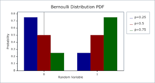
The probabilistic treatment of discrete random variables is comparatively easy: Once a probability is assigned to all different outcomes, the probability of an arbitrary event can be calculated by simply adding the single probabilities. Imagine that in the above example on the S\&P 500 every different payment occurs with the same probability of $25 \%$. Then the probability of losing money by having invested $\$ 50,000$ to purchase the option is $75 \%$, which is the sum of the probabilities of getting either $\$ 0, \$ 10,000$, or $\$ 20,000$ back. In the following sections we provide a short introduction to the most important discrete probability distributions: Bernoulli distribution, binomial distribution, and Poisson distribution. A detailed description together with an introduction to several other discrete probability distributions can be found, for example, in the textbook by Johnson et al. (1993).
金融代写|风险理论投资组合代写Market Risk, Measures and Portfolio 代考|Bernoulli Distribution
We will start the exposition with the Bernoulli distribution. A random variable $X$ is Bernoulli-distributed with parameter $p$ if it has only two possible outcomes, usually encoded as 1 (which might represent success or default) or 0 (which might represent failure or survival).
One classical example for a Bernoulli-distributed random variable occurring in the field of finance is the default event of a company. We observe a company $C$ in a specified time interval $I$, January 1,2007 , until December 31 , 2007. We define
$$
X=\left{\begin{array}{l}
1 \text { if } C \text { defaults in } I \
0 \text { else. }
\end{array}\right.
$$
The parameter $p$ in this case would be the annualized probability of default of company $C$.
In practical applications, we usually do not consider a single company but a whole basket, $C_{1}, \ldots, C_{n}$, of companies. Assuming that all these $n$ companies
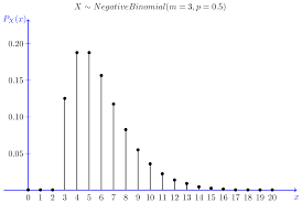
have the same annualized probability of default $p$, this leads to a natural generalization of the Bernoulli distribution called binomial distribution. A binomial distributed random variable $Y$ with parameters $n$ and $p$ is obtained as the sum of $n$ independent ${ }^{5}$ and identically Bernoulli-distributed random variables $X_{1}, \ldots, X_{n}$. In our example, $Y$ represents the total number of defaults occurring in the year 2007 observed for companies $C_{1}, \ldots, C_{n}$. Given the two parameters, the probability of observing $k, 0 \leq k \leq n$ defaults can be explicitly calculated as follows:
$$
P(Y=k)=\left(\begin{array}{l}
n \
k
\end{array}\right) p^{k}(1-p)^{n-k},
$$
where
$$
\left(\begin{array}{l}
n \
k
\end{array}\right)=\frac{n !}{(n-k) ! k !}
$$
Recall that the factorial of a positive integer $n$ is denoted by $n !$ and is equal to $n(n-1)(n-2) \cdots \ldots \cdot 2 \cdot 1$.
Bernoulli distribution and binomial distribution are revisited in Chapter 4 in connection with a fundamental result in the theory of probability called the Central Limit Theorem. Shiryaev (1996) provides a formal discussion of this important result.
风险理论投资组合代写
金融代写|风险理论投资组合代写Market Risk, Measures and Portfolio 代考|BASIC CONCEPTS
随机变量的结果是可能发生的相互排斥的潜在结果。公认的结果符号是希腊字母ω. 样本空间是所有可能结果的集合。样本空间表示为Ω. 给定结果的事实ω一世属于样本空间的表示为ω一世∈Ω. 事件是样本空间的子集,可以表示为一些结果的集合。3例如,考虑微软明年的股票回报。样本空间包含的结果范围从100%(所有投资于微软股票的资金都会损失掉)获得极高的正回报。样本空间可以划分为两个子集:回报小于或等于的结果10%以及回报超过的子集10%. 因此,回报大于10%是一个事件,因为它是样本空间的一个子集。同样,三个月后的一个月 LIBOR 超过4%是一个事件。所有事件的集合通常表示为一种. 在概率论中,我们考虑样本空间Ω连同一组事件一种, 通常写为 (Ω,一种),因为概率的概念与事件相关联。4
金融代写|风险理论投资组合代写Market Risk, Measures and Portfolio 代考|DISCRETE PROBABILITY DISTRIBUTIONS
顾名思义,离散随机变量限制了变量只能采用离散值的结果。例如,考虑一家公司在未来五年内的债务违约。这个随机变量只有两种可能的结果:默认或非默认。因此,它是一个离散随机变量。考虑一个期权合约,其中预付款(即期权价格)为$50,000,合同的买方收到表中给出的付款1.1根据标准普尔 500 指数的回报率从期权卖方处获得。在这种情况下,随机变量是离散随机变量,但结果数量有限。
离散随机变量的概率处理相对容易:一旦将概率分配给所有不同的结果,就可以通过简单地将单个概率相加来计算任意事件的概率。想象一下,在上述标准普尔 500 指数的例子中,每一次不同的支付都以相同的概率发生25%. 然后是因投资而赔钱的概率$50,000购买选项是75%,这是得到任一概率的总和$0,$10,000, 或者$20,000背部。在以下部分中,我们将简要介绍最重要的离散概率分布:伯努利分布、二项分布和泊松分布。例如,可以在 Johnson 等人的教科书中找到详细描述以及对其他几种离散概率分布的介绍。(1993 年)。
金融代写|风险理论投资组合代写Market Risk, Measures and Portfolio 代考|Bernoulli Distribution
我们将从伯努利分布开始阐述。随机变量X是带参数的伯努利分布p如果它只有两种可能的结果,通常编码为 1(可能代表成功或默认)或 0(可能代表失败或生存)。
发生在金融领域的伯努利分布随机变量的一个经典例子是公司的违约事件。我们观察一家公司C在指定的时间间隔内一世,2007 年 1 月 1 日,直到 2007 年 12 月 31 日。我们定义
$$
X=\left{1 如果 C 默认值 一世 0 别的。 \对。
$$
参数p在这种情况下,将是公司违约的年化概率C.
在实际应用中,我们通常不考虑单个公司,而是考虑整个篮子,C1,…,Cn, 公司。假设所有这些n公司
具有相同的年化违约概率p,这导致了伯努利分布的自然推广,称为二项分布。二项分布随机变量是带参数n和p获得为n独立的5和同样伯努利分布的随机变量X1,…,Xn. 在我们的示例中,是表示 2007 年观察到的公司违约总数C1,…,Cn. 给定这两个参数,观察到的概率ķ,0≤ķ≤n默认值可以显式计算如下:
磷(是=ķ)=(n ķ)pķ(1−p)n−ķ,
在哪里
(n ķ)=n!(n−ķ)!ķ!
回想一下正整数的阶乘n表示为n!并且等于n(n−1)(n−2)⋯…⋅2⋅1.
伯努利分布和二项分布在第 4 章中与称为中心极限定理的概率论中的一个基本结果有关。Shiryaev (1996) 对这一重要结果进行了正式讨论。

统计代写请认准statistics-lab™. statistics-lab™为您的留学生涯保驾护航。
金融工程代写
金融工程是使用数学技术来解决金融问题。金融工程使用计算机科学、统计学、经济学和应用数学领域的工具和知识来解决当前的金融问题,以及设计新的和创新的金融产品。
非参数统计代写
非参数统计指的是一种统计方法,其中不假设数据来自于由少数参数决定的规定模型;这种模型的例子包括正态分布模型和线性回归模型。
广义线性模型代考
广义线性模型(GLM)归属统计学领域,是一种应用灵活的线性回归模型。该模型允许因变量的偏差分布有除了正态分布之外的其它分布。
术语 广义线性模型(GLM)通常是指给定连续和/或分类预测因素的连续响应变量的常规线性回归模型。它包括多元线性回归,以及方差分析和方差分析(仅含固定效应)。
有限元方法代写
有限元方法(FEM)是一种流行的方法,用于数值解决工程和数学建模中出现的微分方程。典型的问题领域包括结构分析、传热、流体流动、质量运输和电磁势等传统领域。
有限元是一种通用的数值方法,用于解决两个或三个空间变量的偏微分方程(即一些边界值问题)。为了解决一个问题,有限元将一个大系统细分为更小、更简单的部分,称为有限元。这是通过在空间维度上的特定空间离散化来实现的,它是通过构建对象的网格来实现的:用于求解的数值域,它有有限数量的点。边界值问题的有限元方法表述最终导致一个代数方程组。该方法在域上对未知函数进行逼近。[1] 然后将模拟这些有限元的简单方程组合成一个更大的方程系统,以模拟整个问题。然后,有限元通过变化微积分使相关的误差函数最小化来逼近一个解决方案。
tatistics-lab作为专业的留学生服务机构,多年来已为美国、英国、加拿大、澳洲等留学热门地的学生提供专业的学术服务,包括但不限于Essay代写,Assignment代写,Dissertation代写,Report代写,小组作业代写,Proposal代写,Paper代写,Presentation代写,计算机作业代写,论文修改和润色,网课代做,exam代考等等。写作范围涵盖高中,本科,研究生等海外留学全阶段,辐射金融,经济学,会计学,审计学,管理学等全球99%专业科目。写作团队既有专业英语母语作者,也有海外名校硕博留学生,每位写作老师都拥有过硬的语言能力,专业的学科背景和学术写作经验。我们承诺100%原创,100%专业,100%准时,100%满意。
随机分析代写
随机微积分是数学的一个分支,对随机过程进行操作。它允许为随机过程的积分定义一个关于随机过程的一致的积分理论。这个领域是由日本数学家伊藤清在第二次世界大战期间创建并开始的。
时间序列分析代写
随机过程,是依赖于参数的一组随机变量的全体,参数通常是时间。 随机变量是随机现象的数量表现,其时间序列是一组按照时间发生先后顺序进行排列的数据点序列。通常一组时间序列的时间间隔为一恒定值(如1秒,5分钟,12小时,7天,1年),因此时间序列可以作为离散时间数据进行分析处理。研究时间序列数据的意义在于现实中,往往需要研究某个事物其随时间发展变化的规律。这就需要通过研究该事物过去发展的历史记录,以得到其自身发展的规律。
回归分析代写
多元回归分析渐进(Multiple Regression Analysis Asymptotics)属于计量经济学领域,主要是一种数学上的统计分析方法,可以分析复杂情况下各影响因素的数学关系,在自然科学、社会和经济学等多个领域内应用广泛。
MATLAB代写
MATLAB 是一种用于技术计算的高性能语言。它将计算、可视化和编程集成在一个易于使用的环境中,其中问题和解决方案以熟悉的数学符号表示。典型用途包括:数学和计算算法开发建模、仿真和原型制作数据分析、探索和可视化科学和工程图形应用程序开发,包括图形用户界面构建MATLAB 是一个交互式系统,其基本数据元素是一个不需要维度的数组。这使您可以解决许多技术计算问题,尤其是那些具有矩阵和向量公式的问题,而只需用 C 或 Fortran 等标量非交互式语言编写程序所需的时间的一小部分。MATLAB 名称代表矩阵实验室。MATLAB 最初的编写目的是提供对由 LINPACK 和 EISPACK 项目开发的矩阵软件的轻松访问,这两个项目共同代表了矩阵计算软件的最新技术。MATLAB 经过多年的发展,得到了许多用户的投入。在大学环境中,它是数学、工程和科学入门和高级课程的标准教学工具。在工业领域,MATLAB 是高效研究、开发和分析的首选工具。MATLAB 具有一系列称为工具箱的特定于应用程序的解决方案。对于大多数 MATLAB 用户来说非常重要,工具箱允许您学习和应用专业技术。工具箱是 MATLAB 函数(M 文件)的综合集合,可扩展 MATLAB 环境以解决特定类别的问题。可用工具箱的领域包括信号处理、控制系统、神经网络、模糊逻辑、小波、仿真等。