如果你也在 怎样代写风险理论投资组合这个学科遇到相关的难题,请随时右上角联系我们的24/7代写客服。
为了衡量市场风险,投资者和分析师使用风险值(VaR)方法。风险值建模是一种统计风险管理方法,它可以量化股票或投资组合的潜在损失,以及该潜在损失发生的概率。
statistics-lab™ 为您的留学生涯保驾护航 在代写风险理论投资组合方面已经树立了自己的口碑, 保证靠谱, 高质且原创的统计Statistics代写服务。我们的专家在代写风险理论投资组合代写方面经验极为丰富,各种代写风险理论投资组合相关的作业也就用不着说。
我们提供的风险理论投资组合及其相关学科的代写,服务范围广, 其中包括但不限于:
- Statistical Inference 统计推断
- Statistical Computing 统计计算
- Advanced Probability Theory 高等概率论
- Advanced Mathematical Statistics 高等数理统计学
- (Generalized) Linear Models 广义线性模型
- Statistical Machine Learning 统计机器学习
- Longitudinal Data Analysis 纵向数据分析
- Foundations of Data Science 数据科学基础

金融代写|风险理论投资组合代写Market Risk, Measures and Portfolio 代考|Covariance and Correlation
There are two strongly related measures among many that are commonly used to measure how two random variables tend to move together, the covariance and the correlation. Letting:
$\sigma_{X}$ denote the standard deviation of $X$.
$\sigma_{Y}$ denote the standard deviation of $Y$.
$\sigma_{X Y}$ denote the covariance between $X$ and $Y$.
$\rho_{X Y}$ denote the correlation between $X$ and $Y$.
The relationship between the correlation, which is also denoted by $\rho_{X Y}$ $=\operatorname{corr}(X, Y)$, and covariance is as follows:
$$
\rho_{X Y}=\frac{\sigma_{X Y}}{\sigma_{X} \sigma_{Y}} .
$$
Here the covariance, also denoted by $\sigma_{X Y}=\operatorname{cov}(X, Y)$, is defined as
$$
\begin{aligned}
\sigma_{X Y} &=E(X-E X)(Y-E Y) \
&=E(X Y)-E X E Y
\end{aligned}
$$
It can be shown that the correlation can only have values from $-1$ to $+1$. When the correlation is zero, the two random variables are said to be uncorrelated.
If we add two random variables, $X+Y$, the expected value (first central moment) is simply the sum of the expected value of the two random variables. That is,
$$
E(X+Y)=E X+E Y .
$$
The variance of the sum of two random variables, denoted by $\sigma_{X+Y}^{2}$, is
$$
\sigma_{X+Y}^{2}=\sigma_{X}^{2}+\sigma_{Y}^{2}+2 \sigma_{X Y} .
$$
Here the last term accounts for the fact that there might be a dependence between $X$ and $Y$ measured through the covariance. In Chapter 8, we consider the variance of the portfolio return of $n$ assets which is expressed by means of the variances of the assets’ returns and the covariances between them.
金融代写|风险理论投资组合代写Market Risk, Measures and Portfolio 代考|Multivariate Normal Distribution
In finance, it is common to assume that the random variables are normally distributed. The joint distribution is then referred to as a multivariate normal
distribution. ${ }^{13}$ We provide an explicit representation of the density function of a general multivariate normal distribution.
Consider first $n$ independent standard normal random variables $X_{1}, \ldots$, $X_{n}$. Their common density function can be written as the product of their individual density functions and so we obtain the following expression as the density function of the random vector $X=X_{1}, \ldots, X_{n}$ :
$$
f_{\mathrm{X}}\left(x_{1}, \ldots, x_{n}\right)=\frac{1}{(\sqrt{2 \pi})^{n}} e^{-\frac{x^{\prime} x}{2}},
$$
where the vector notation $x^{\prime} x$ denotes the sum of the components of the vector $x$ raised to the second power, $x^{\prime} x=\sum_{i=1}^{n} x_{i}^{2}$.
Now consider $n$ vectors with $n$ real components arranged in a matrix $A$. In this case, it is often said that the matrix $A$ has a $n \times n$ dimension. The random variable
$$
Y=A X+\mu,
$$
in which $A X$ denotes the $n \times n$ matrix $A$ multiplied by the random vector $X$ and $\mu$ is a vector of $n$ constants, has a general multivariate normal distribution. The density function of $Y$ can now be expressed as ${ }^{14}$
where $|\Sigma|$ denotes the determinant of the matrix $\Sigma$ and $\Sigma^{-1}$ denotes the inverse of $\Sigma$. The matrix $\Sigma$ can be calculated from the matrix $A, \Sigma=A A^{\prime}$. The elements of $\Sigma=\left{\sigma_{i j}\right}_{i, j-1}^{n}$ are the covariances between the components of the vector $Y$,
$$
\sigma_{i j}=\operatorname{cov}\left(Y_{i}, Y_{j}\right) .
$$
Figure $1.5$ contains a plot of the probability density function of a two-dimensional normal distribution with a covariance matrix,
$$
\Sigma=\left(\begin{array}{cc}
1 & 0.8 \
0.8 & 1
\end{array}\right)
$$
and mean $\mu=(0,0)$. The matrix $A$ from the representation given in formula (1.3) equals
$$
A=\left(\begin{array}{cc}
1 & 0 \
0.8 & 0.6
\end{array}\right)
$$
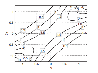
The correlation between the two components of the random vector $Y$ is equal to $0.8, \operatorname{corr}\left(Y_{1}, Y_{2}\right)=0.8$ because in this example the variances of the two components are equal to 1 . This is a strong positive correlation, which means that the realizations of the random vector $Y$ clusters along the diagonal splitting the first and the third quadrant. This is illustrated in Figure 1.6, which shows the contour lines of the two-dimensional density function plotted in Figure 1.5. The contour lines are ellipses centered at the mean $\mu=(0,0)$ of the random vector $Y$ with their major axes lying along the diagonal of the first quadrant. The contour lines indicate that realizations of the random vector $Y$ roughly take the form of an elongated ellipse as the ones shown in Figure 1.6, which means that large values of $Y_{1}$ will correspond to large values of $Y_{2}$ in a given pair of observations.
金融代写|风险理论投资组合代写Market Risk, Measures and Portfolio 代考|Copula Functions
Correlation is a widespread concept in modern finance and risk management and stands for a measure of dependence between random variables. However, this term is often incorrectly used to mean any notion of dependence. Actually, correlation is one particular measure of dependence among many. In the world of multivariate normal distribution and more generally in the world of spherical and elliptical distributions, it is the accepted measure.
A major drawback of correlation is that it is not invariant under nonlinear strictly increasing transformations. In general,
$$
\operatorname{corr}(T(X), T(Y)) \neq \operatorname{corr}(X, Y)
$$
where $T(x)$ is such transformation. One example which explains this technical requirement is the following: Assume that $X$ and $Y$ represent the continuous return (log-return) of two assets over the period $[0, t]$, where $t$ denotes some point of time in the future. If you know the correlation of these two random variables, this does not imply that you know the dependence structure between the asset prices itself because the asset prices $\left(P\right.$ and $Q$ for asset $X$ and $Y$, respectively) are obtained by $P_{t}=P_{0} \exp (X)$ and $Q_{t}=Q_{0} \exp (Y)$, where $P_{0}$ and $Q_{0}$ denote the corresponding asset prices at time 0 . The asset prices are strictly increasing functions of the return but the correlation structure is not maintained by this transformation. This observation implies that the return could be uncorrelated whereas the prices are strongly correlated and vice versa.
A more prevalent approach that overcomes this disadvantage is to model dependency using copulas. As noted by Patton (2004, p. 3), “The word copula comes from Latin for a ‘link’ or ‘bond,’ and was coined by Sklar (1959), who first proved the theorem that a collection of marginal distributions can be ‘coupled’ together via a copula to form a multivariate distribution.” The idea is as follows. The description of the joint distribution of a random vector is divided into two parts:
- The specification of the marginal distributions.
- the specification of the dependence structure by means of a special function, called copula.
The use of copulas ${ }^{19}$ offers the following advantages:
- The nature of dependency that can be modeled is more general. In comparison, only linear dependence can be explained by the correlation.
- Dependence of extreme events might be modeled.
- Copulas are indifferent to continuously increasing transformations (not only linear as it is true for correlations).
From a mathematical viewpoint, a copula function $C$ is nothing more than a probability distribution function on the $n$-dimensional hypercube $I_{n}=[0,1] \times[0,1] \times \ldots \times[0,1]:$
$$
\begin{aligned}
C: I_{n} & \rightarrow[0,1] \
\left(u_{1}, \ldots, u_{n}\right) & \rightarrow C\left(u_{1}, \ldots, u_{n}\right)
\end{aligned}
$$
It has been shown ${ }^{20}$ that any multivariate probability distribution function $F_{Y}$ of some random vector $Y=\left(Y_{1}, \ldots, Y_{n}\right)$ can be represented with the help of a copula function $C$ in the following form:
$$
\begin{aligned}
F_{Y}\left(y_{1}, \ldots, y_{n}\right) &=P\left(Y_{1} \leq y_{1}, \ldots, Y_{n} \leq y_{n}\right)=C\left(P\left(Y_{1} \leq y_{1}\right), \ldots, P\left(Y_{n} \leq y_{n}\right)\right) \
&=C\left(F_{Y_{1}}\left(y_{1}\right), \ldots, F_{Y_{n}}\left(y_{n}\right)\right)
\end{aligned}
$$
where $F_{Y_{i}}\left(y_{i}\right), i=1, \ldots, n$ denote the marginal distribution functions of the random variables $Y_{i}, i=1, \ldots, n$.
风险理论投资组合代写
金融代写|风险理论投资组合代写Market Risk, Measures and Portfolio 代考|Covariance and Correlation
在许多通常用于衡量两个随机变量如何趋于一起移动的度量中,有两个密切相关的度量,即协方差和相关性。出租:
σX表示标准差X.
σ是表示标准差是.
σX是表示之间的协方差X和是.
ρX是表示之间的相关性X和是.
相关性之间的关系,也表示为ρX是 =更正(X,是), 协方差如下:
ρX是=σX是σXσ是.
这里的协方差也表示为σX是=这(X,是), 定义为
σX是=和(X−和X)(是−和是) =和(X是)−和X和是
可以证明,相关性只能具有来自−1到+1. 当相关性为零时,称这两个随机变量不相关。
如果我们添加两个随机变量,X+是,期望值(第一中心矩)只是两个随机变量的期望值之和。那是,
和(X+是)=和X+和是.
两个随机变量之和的方差,表示为σX+是2, 是
σX+是2=σX2+σ是2+2σX是.
在这里,最后一项解释了这样一个事实,即两者之间可能存在依赖关系X和是通过协方差测量。在第 8 章中,我们考虑了投资组合收益的方差n用资产收益的方差和它们之间的协方差来表示的资产。
金融代写|风险理论投资组合代写Market Risk, Measures and Portfolio 代考|Multivariate Normal Distribution
在金融领域,通常假设随机变量是正态分布的。然后将联合分布称为多元正态分布
分配。13我们提供了一般多元正态分布的密度函数的显式表示。
先考虑n独立标准正态随机变量X1,…, Xn. 它们的共同密度函数可以写成它们各自密度函数的乘积,因此我们得到以下表达式作为随机向量的密度函数X=X1,…,Xn :
FX(X1,…,Xn)=1(2圆周率)n和−X′X2,
其中向量表示法X′X表示向量的分量之和X提升到二次方,X′X=∑一世=1nX一世2.
现在考虑n向量与n排列成矩阵的实分量一种. 在这种情况下,人们常说矩阵一种有一个n×n方面。随机变量
是=一种X+μ,
其中一种X表示n×n矩阵一种乘以随机向量X和μ是一个向量n常数,具有一般的多元正态分布。的密度函数是现在可以表示为14
在哪里|Σ|表示矩阵的行列式Σ和Σ−1表示的倒数Σ. 矩阵Σ可以从矩阵计算一种,Σ=一种一种′. 的元素\Sigma=\left{\sigma_{i j}\right}_{i, j-1}^{n}\Sigma=\left{\sigma_{i j}\right}_{i, j-1}^{n}是向量分量之间的协方差是,
σ一世j=这(是一世,是j).
数字1.5包含具有协方差矩阵的二维正态分布的概率密度函数图,
Σ=(10.8 0.81)
和意思μ=(0,0). 矩阵一种从公式(1.3)中给出的表示等于
一种=(10 0.80.6)
随机向量的两个分量之间的相关性是等于0.8,更正(是1,是2)=0.8因为在这个例子中,两个分量的方差等于 1 。这是一个强正相关,这意味着随机向量的实现是沿着分割第一象限和第三象限的对角线簇。这如图 1.6 所示,它显示了图 1.5 中绘制的二维密度函数的等高线。等高线是以均值为中心的椭圆μ=(0,0)随机向量的是它们的主轴位于第一象限的对角线上。等高线表明随机向量的实现是大致采用如图 1.6 所示的拉长椭圆的形式,这意味着较大的值是1将对应于较大的值是2在给定的一对观察中。
金融代写|风险理论投资组合代写Market Risk, Measures and Portfolio 代考|Copula Functions
相关性是现代金融和风险管理中的一个广泛概念,代表随机变量之间依赖关系的度量。然而,这个术语经常被错误地用来表示任何依赖的概念。实际上,相关性是衡量许多人之间依赖关系的一种特殊方法。在多元正态分布的世界中,更一般地在球形和椭圆分布的世界中,它是公认的度量。
相关性的一个主要缺点是它在非线性严格递增变换下不是不变的。一般来说,
更正(吨(X),吨(是))≠更正(X,是)
在哪里吨(X)就是这样的转变。一个解释此技术要求的示例如下: 假设X和是表示该期间内两种资产的连续回报(对数回报)[0,吨], 在哪里吨表示未来的某个时间点。如果您知道这两个随机变量的相关性,这并不意味着您知道资产价格本身之间的依赖结构,因为资产价格(磷和问对于资产X和是, 分别) 由下式获得磷吨=磷0经验(X)和问吨=问0经验(是), 在哪里磷0和问0表示时间 0 的相应资产价格。资产价格是收益的严格递增函数,但这种转换并不能维持相关结构。这一观察表明,回报可能不相关,而价格密切相关,反之亦然。
克服这个缺点的更普遍的方法是使用 copula 对依赖关系进行建模。正如 Patton (2004, p. 3) 所指出的,“copula 这个词来自拉丁语中的‘链接’或‘键’,由 Sklar (1959) 创造,他首先证明了边际分布的集合可以通过 copula 将它们“耦合”在一起以形成多元分布。” 思路如下。随机向量联合分布的描述分为两部分:
- 边际分布的规范。
- 通过称为 copula 的特殊函数指定依赖结构。
copula 的使用19提供以下优势:
- 可以建模的依赖性的性质更普遍。相比之下,相关性只能解释线性相关性。
- 极端事件的依赖性可能会被建模。
- Copulas 对不断增加的转换无动于衷(不仅是线性的,因为它对相关性也是如此)。
从数学的角度来看,copula 函数C只不过是一个概率分布函数n维超立方体一世n=[0,1]×[0,1]×…×[0,1]:
C:一世n→[0,1] (在1,…,在n)→C(在1,…,在n)
已经显示20任何多元概率分布函数F是一些随机向量是=(是1,…,是n)可以在 copula 函数的帮助下表示C采用以下形式:
F是(是1,…,是n)=磷(是1≤是1,…,是n≤是n)=C(磷(是1≤是1),…,磷(是n≤是n)) =C(F是1(是1),…,F是n(是n))
在哪里F是一世(是一世),一世=1,…,n表示随机变量的边际分布函数是一世,一世=1,…,n.

统计代写请认准statistics-lab™. statistics-lab™为您的留学生涯保驾护航。
金融工程代写
金融工程是使用数学技术来解决金融问题。金融工程使用计算机科学、统计学、经济学和应用数学领域的工具和知识来解决当前的金融问题,以及设计新的和创新的金融产品。
非参数统计代写
非参数统计指的是一种统计方法,其中不假设数据来自于由少数参数决定的规定模型;这种模型的例子包括正态分布模型和线性回归模型。
广义线性模型代考
广义线性模型(GLM)归属统计学领域,是一种应用灵活的线性回归模型。该模型允许因变量的偏差分布有除了正态分布之外的其它分布。
术语 广义线性模型(GLM)通常是指给定连续和/或分类预测因素的连续响应变量的常规线性回归模型。它包括多元线性回归,以及方差分析和方差分析(仅含固定效应)。
有限元方法代写
有限元方法(FEM)是一种流行的方法,用于数值解决工程和数学建模中出现的微分方程。典型的问题领域包括结构分析、传热、流体流动、质量运输和电磁势等传统领域。
有限元是一种通用的数值方法,用于解决两个或三个空间变量的偏微分方程(即一些边界值问题)。为了解决一个问题,有限元将一个大系统细分为更小、更简单的部分,称为有限元。这是通过在空间维度上的特定空间离散化来实现的,它是通过构建对象的网格来实现的:用于求解的数值域,它有有限数量的点。边界值问题的有限元方法表述最终导致一个代数方程组。该方法在域上对未知函数进行逼近。[1] 然后将模拟这些有限元的简单方程组合成一个更大的方程系统,以模拟整个问题。然后,有限元通过变化微积分使相关的误差函数最小化来逼近一个解决方案。
tatistics-lab作为专业的留学生服务机构,多年来已为美国、英国、加拿大、澳洲等留学热门地的学生提供专业的学术服务,包括但不限于Essay代写,Assignment代写,Dissertation代写,Report代写,小组作业代写,Proposal代写,Paper代写,Presentation代写,计算机作业代写,论文修改和润色,网课代做,exam代考等等。写作范围涵盖高中,本科,研究生等海外留学全阶段,辐射金融,经济学,会计学,审计学,管理学等全球99%专业科目。写作团队既有专业英语母语作者,也有海外名校硕博留学生,每位写作老师都拥有过硬的语言能力,专业的学科背景和学术写作经验。我们承诺100%原创,100%专业,100%准时,100%满意。
随机分析代写
随机微积分是数学的一个分支,对随机过程进行操作。它允许为随机过程的积分定义一个关于随机过程的一致的积分理论。这个领域是由日本数学家伊藤清在第二次世界大战期间创建并开始的。
时间序列分析代写
随机过程,是依赖于参数的一组随机变量的全体,参数通常是时间。 随机变量是随机现象的数量表现,其时间序列是一组按照时间发生先后顺序进行排列的数据点序列。通常一组时间序列的时间间隔为一恒定值(如1秒,5分钟,12小时,7天,1年),因此时间序列可以作为离散时间数据进行分析处理。研究时间序列数据的意义在于现实中,往往需要研究某个事物其随时间发展变化的规律。这就需要通过研究该事物过去发展的历史记录,以得到其自身发展的规律。
回归分析代写
多元回归分析渐进(Multiple Regression Analysis Asymptotics)属于计量经济学领域,主要是一种数学上的统计分析方法,可以分析复杂情况下各影响因素的数学关系,在自然科学、社会和经济学等多个领域内应用广泛。
MATLAB代写
MATLAB 是一种用于技术计算的高性能语言。它将计算、可视化和编程集成在一个易于使用的环境中,其中问题和解决方案以熟悉的数学符号表示。典型用途包括:数学和计算算法开发建模、仿真和原型制作数据分析、探索和可视化科学和工程图形应用程序开发,包括图形用户界面构建MATLAB 是一个交互式系统,其基本数据元素是一个不需要维度的数组。这使您可以解决许多技术计算问题,尤其是那些具有矩阵和向量公式的问题,而只需用 C 或 Fortran 等标量非交互式语言编写程序所需的时间的一小部分。MATLAB 名称代表矩阵实验室。MATLAB 最初的编写目的是提供对由 LINPACK 和 EISPACK 项目开发的矩阵软件的轻松访问,这两个项目共同代表了矩阵计算软件的最新技术。MATLAB 经过多年的发展,得到了许多用户的投入。在大学环境中,它是数学、工程和科学入门和高级课程的标准教学工具。在工业领域,MATLAB 是高效研究、开发和分析的首选工具。MATLAB 具有一系列称为工具箱的特定于应用程序的解决方案。对于大多数 MATLAB 用户来说非常重要,工具箱允许您学习和应用专业技术。工具箱是 MATLAB 函数(M 文件)的综合集合,可扩展 MATLAB 环境以解决特定类别的问题。可用工具箱的领域包括信号处理、控制系统、神经网络、模糊逻辑、小波、仿真等。