如果你也在 怎样代写密码学Cryptography & Cryptanalysis这个学科遇到相关的难题,请随时右上角联系我们的24/7代写客服。
密码学创造了具有隐藏意义的信息;密码分析是破解这些加密信息以恢复其意义的科学。许多人用密码学一词来代替密码学;然而,重要的是要记住,密码学包括了密码学和密码分析。
statistics-lab™ 为您的留学生涯保驾护航 在代写密码学Cryptography & Cryptanalysis方面已经树立了自己的口碑, 保证靠谱, 高质且原创的统计Statistics代写服务。我们的专家在代写密码学Cryptography & Cryptanalysis代写方面经验极为丰富,各种代写密码学Cryptography & Cryptanalysis相关的作业也就用不着说。
我们提供的密码学Cryptography & Cryptanalysis及其相关学科的代写,服务范围广, 其中包括但不限于:
- Statistical Inference 统计推断
- Statistical Computing 统计计算
- Advanced Probability Theory 高等概率论
- Advanced Mathematical Statistics 高等数理统计学
- (Generalized) Linear Models 广义线性模型
- Statistical Machine Learning 统计机器学习
- Longitudinal Data Analysis 纵向数据分析
- Foundations of Data Science 数据科学基础
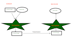
数学代写|密码学作业代写Cryptography & Cryptanalysis代考|Deterministic Visual Cryptography
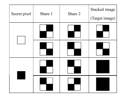
A simple example is shown in Fig. 2.1. When sharing a white pixel $s=0$, one randomly chooses one row from the second and the third rows in Fig. 2.1, and distributes the second column to Share 1 and the third column to Share 2. The final stacking result is a $2 \times 2$ block with two black pixels, as shown in the last column. Similarly, while sharing a black pixel $s=1$, one randomly chooses one row from the fourth and the fifth rows of the table, and distributes the second column to Share 1 and the third column to Share 2 . The final stacking result is a $2 \times 2$ block with four black pixels, as shown in the last column. So, one secret pixel is expanded to a block having four pixels, or equivalently, one secret pixel is represented by four sub-pixels.
If we look at one share, no matter whether a white pixel is shared or a black pixel is shared, we always see roughly equal number of the following two types of blocks on each share:
$$
\mathbf{A}{1}=\left[\begin{array}{ll} 0 & 1 \ 1 & 0 \end{array}\right], \quad \mathbf{A}{2}=\left[\begin{array}{ll}
1 & 0 \
0 & 1
\end{array}\right]
$$
Thus, by checking only one share, it is impossible to tell if a black pixel is shared or a white pixel is shared. This is the security consideration in visual cryptography. But
if we check the target image, the block corresponding to white secret pixel has two black pixels, while the block corresponding to the black secret pixel has four black pixels. Thus, one can distinguish between the black region and the white region of the secret image by checking the target image. This is the contrast consideration in visual cryptography.
When designing a deterministic VC algorithm, the blocks corresponding to a secret pixel are usually vectorized and organized into a matrix. For example, the two blocks in (2.5) are represented as a matrix
$$
\mathbf{C}=\left[\begin{array}{c}
\operatorname{vec}\left(\mathbf{A}{1}\right)^{T} \ \operatorname{vec}\left(\mathbf{A}{2}\right)^{T}
\end{array}\right]
$$
where each block $\mathbf{A}{i}, i=1,2$, is stretched to a column vector by function vec $\left(\mathbf{A}{i}\right)$, transposed, and filled into one row of $\mathbf{C}$. So, each row of $\mathbf{C}$ should be distributed to one share and then reshaped to appropriate shape. For the design of VC algorithm, the reshaping is not a central issue. So, it is usually omitted when defining the $V C$.
For the example in Fig. 2.1, we have the following matrices:
$$
\begin{aligned}
&\mathbf{C}{0}=\left{\mathbf{C}{1}^{0}, \mathbf{C}{2}^{0}\right}=\left{\left[\begin{array}{llll} 0 & 1 & 1 & 0 \ 0 & 1 & 1 & 0 \end{array}\right],\left[\begin{array}{llll} 1 & 0 & 0 & 1 \ 1 & 0 & 0 & 1 \end{array}\right]\right} \ &\mathbf{C}{1}=\left{\mathbf{C}{1}^{1}, \mathbf{C}{2}^{1}\right}=\left{\left[\begin{array}{llll}
0 & 1 & 1 & 0 \
1 & 0 & 0 & 1
\end{array}\right],\left[\begin{array}{llll}
1 & 0 & 0 & 1 \
0 & 1 & 1 & 0
\end{array}\right]\right}
\end{aligned}
$$
数学代写|密码学作业代写Cryptography & Cryptanalysis代考|Definition
Let $\mathcal{H}(\mathbf{v})$ be the Hamming weight of a Boolean vector $\mathbf{v}$, i.e., the number of $1 \mathrm{~s}$ in $\mathbf{v}$. Based on the above explanation, the $(k, n)$-threshold VC can be formally defined by the following definition [13]:
Definition 2.1 $(k, n)$-threshold VC: $\mathrm{A}(k, n)$-threshold VC consists of two collections of $n \times m$ matrices $\mathrm{C}{0}$ and $\mathrm{C}{1}$. To share a white (black resp.) pixel, one randomly chooses one matrix from $\mathrm{C}{0}\left(\mathrm{C}{1}\right.$ resp.). Each row of the chosen matrix is distributed to one share. The following two conditions should be satisfied:
- Contrast condition: For any $\mathbf{C} \in \mathbf{C}{0}$, let $\mathbf{C}=\left[\mathbf{c}{1}^{T}, \ldots, \mathbf{c}{n}^{T}\right]^{T}$, where $\mathbf{c}{i}$ is the $i$-th row of matrix $C$. Then, the stacking of any $k$ rows or more satisfies $\mathcal{H}\left(\vee_{j=1}^{k} \mathbf{c}{i{j}}\right) \leq d-\alpha$, where $i_{1}, \ldots, i_{k}$ are $k$ randomly chosen row indices. For any $\mathbf{C} \in \mathrm{C}{1}, \mathcal{H}\left(\mathrm{V}{j=1}^{k} \mathbf{c}{i{j}}\right) \geq d$.
- Security condition: For any $q<k$ randomly chosen shares $\left{i_{1}, \ldots, i_{q}\right} \in$ ${1,2, \ldots, n}$, the two collections of matrices $\hat{C}{0}$ and $\hat{C}{1}$, obtained by restricting each matrix to the rows $i_{1}, \ldots, i_{q}$, should be indistinguishable. Namely, $\hat{\mathrm{C}}{0}$ and $\hat{C}{1}$ should contain the same matrices with the same frequencies.
The parameter $m$ is pixel expansion rate and parameter a gives the minimum difference in Hamming weight between the stacking result for a black secret pixel and the stacking result for a white secret pixel.
数学代写|密码学作业代写Cryptography & Cryptanalysis代考|Constructions
The construction of the two sets of matrices $C_{0}$ and $C_{1}$ can be based on two basis matrices $\mathbf{B}{0}$ and $\mathbf{B}{1}$. After designing $\mathbf{B}{0}\left(\mathbf{B}{1}\right.$ resp.), $\mathbf{C}{0}$ may include all column permutations of $\mathbf{B}{0} \mathrm{~ ( B ⿱}$ corresponding $\mathrm{C}_{0}$.
One optimal construction for $(n, n)$-threshold scheme was proposed by Naor and Shamir [13]. It starts with a set having $n$ components, which is called a ground set. Let the set be $\mathrm{W}=\left{e_{1}, \ldots, e_{n}\right}$, which has $2^{n}$ subsets. Among these subsets, let $U_{1}, \ldots, U_{2^{w-1}}$ be the $2^{n-1}$ subsets with even cardinality, and let $V_{1}, \ldots, V_{2^{w-1}}$ be the $2^{n-1}$ subsets with odd cardinality. Then we obtain two basis matrices $\mathbf{B}{0}$ and $\mathbf{B}{1}$ as follows:
$$
\begin{aligned}
&B_{0}[i, j]= \begin{cases}1, & \text { if } e_{i} \in \mathrm{U}{j} \ 0, & \text { otherwise. }\end{cases} \ &B{1}[i, j]= \begin{cases}1, & \text { if } e_{i} \in \mathrm{V}{j} \ 0, & \text { otherwise. }\end{cases} \end{aligned} $$ Then the set of matrices $C{0}\left(C_{1}\right.$ resp.) is obtained by all possible column permutations of $\mathbf{B}{0}$ ( $\mathbf{B}{1}$ resp.).
For example, Let $n=3$ and $m=4$, then we use the ground set $\mathrm{W}=\left{e_{1}, e_{2}, e_{3}\right}$. So, we have the following subsets:
$$
\begin{aligned}
&\mathrm{U}{1}=\left{e{1}, e_{2}\right}, \quad \mathrm{U}{2}=\left{e{1}, e_{3}\right}, \quad \mathrm{U}{3}=\left{e{2}, e_{3}\right}, \quad \mathrm{U}{4}=\emptyset \ &\mathrm{V}{1}=\left{e_{1}\right}, \quad \mathrm{V}{2}=\left{e{2}\right}, \quad \mathrm{V}{3}=\left{e{3}\right}, \quad \mathrm{V}{4}=\left{e{1}, e_{2}, e_{3}\right}
\end{aligned}
$$
From (2.10), we get two basis matrices:
$$
\mathbf{B}{0}=\left[\begin{array}{llll} 1 & 1 & 0 & 0 \ 1 & 0 & 1 & 0 \ 0 & 1 & 1 & 0 \end{array}\right], \quad \mathbf{B}{1}=\left[\begin{array}{llll}
1 & 0 & 0 & 1 \
0 & 1 & 0 & 1 \
0 & 0 & 1 & 1
\end{array}\right]
$$
The set of matrices $\mathrm{C}{0}\left(\mathrm{C}{1}\right.$ resp.) contains $2^{n-1} !=4 !=24$ matrices that are all possible column permutations of the matrix $\mathbf{B}{0}\left(\mathbf{B}{1}\right.$ resp.).
Naor and Shamir proved that this scheme is optimal, in that it has the minimum pixel expansion $m$ and maximum contrast $\alpha$ for a given $n$ :
Theorem $2.1$ ([13]) For any ( $n, n)$-threshold deterministic VC, the contrast is upper bounded by $1 / 2^{n-1}$, and the pixel expansion $m$ is lower bounded by $2^{n-1}$.
Proof for security and contrast condition can be found in [13], which is thus omitted here. We also direct the reader to $[13]$ for more general constructions such as $(k, n)$-threshold scheme.
An experimental result using the scheme in Fig. 2.1 is shown in Fig. 2.2.
密码学代写
数学代写|密码学作业代写Cryptography & Cryptanalysis代考|Deterministic Visual Cryptography
一个简单的例子如图 2.1 所示。共享白色像素时s=0,从图 2.1 的第二行和第三行中随机选择一行,将第二列分配给 Share 1,将第三列分配给 Share 2。最终的堆叠结果是2×2块有两个黑色像素,如最后一列所示。同样,同时共享一个黑色像素s=1,从表格的第四行和第五行中随机选择一行,将第二列分配给 Share 1 ,将第三列分配给 Share 2 。最终的堆叠结果是2×2具有四个黑色像素的块,如最后一列所示。因此,一个秘密像素被扩展为具有四个像素的块,或者等效地,一个秘密像素由四个子像素表示。
如果我们看一个共享,无论是共享白色像素还是共享黑色像素,我们总是在每个共享上看到大致相同数量的以下两种类型的块:
一种1=[01 10],一种2=[10 01]
因此,仅通过检查一个共享,无法判断是共享黑色像素还是共享白色像素。这是视觉密码学中的安全考虑。但
如果我们检查目标图像,白色秘密像素对应的块有两个黑色像素,而黑色秘密像素对应的块有四个黑色像素。因此,可以通过检查目标图像来区分秘密图像的黑色区域和白色区域。这是视觉密码学中的对比考虑。
在设计确定性 VC 算法时,通常将与秘密像素对应的块矢量化并组织成矩阵。例如,(2.5)中的两个块表示为一个矩阵
C=[一个东西(一种1)吨 一个东西(一种2)吨]
每个块在哪里一种一世,一世=1,2, 被函数 vec 拉伸成列向量(一种一世),转置并填充到一排C. 所以,每一行C应分配到一份,然后重新塑造成适当的形状。对于 VC 算法的设计,重塑不是核心问题。因此,通常在定义在C.
对于图 2.1 中的示例,我们有以下矩阵:
\begin{对齐} &\mathbf{C}{0}=\left{\mathbf{C}{1}^{0}, \mathbf{C}{2}^{0}\right}=\left{ \left[\begin{array}{llll}0&1&1&0\0&1&1&0 \end{array}\right],\left[\begin{array}{llll}1&0&0 0&1\1&0&0&1\end{array}\right]\right}\ &\mathbf{C}{1}=\left{\mathbf{C}{1}^{1},\mathbf{C}{2}^{1}\right}=\left{\left[\begin {array}{llll}0&1&1&0\1&0&0&1\end{array}\right],\left[\begin{array}{llll}1&0&0&1\0&1&1&0\end{array}\right]\right}\end{aligned}\begin{对齐} &\mathbf{C}{0}=\left{\mathbf{C}{1}^{0}, \mathbf{C}{2}^{0}\right}=\left{ \left[\begin{array}{llll}0&1&1&0\0&1&1&0 \end{array}\right],\left[\begin{array}{llll}1&0&0 0&1\1&0&0&1\end{array}\right]\right}\ &\mathbf{C}{1}=\left{\mathbf{C}{1}^{1},\mathbf{C}{2}^{1}\right}=\left{\left[\begin {array}{llll}0&1&1&0\1&0&0&1\end{array}\right],\left[\begin{array}{llll}1&0&0&1\0&1&1&0\end{array}\right]\right}\end{aligned}
数学代写|密码学作业代写Cryptography & Cryptanalysis代考|Definition
让H(在)是布尔向量的汉明权重在,即数量1 s在在. 基于以上解释,(ķ,n)-阈值 VC 可以由以下定义 [13] 正式定义:
定义 2.1(ķ,n)-阈值 VC:一种(ķ,n)-threshold VC 由两个集合组成n×米矩阵C0和C1. 为了共享一个白色(黑色)像素,一个随机选择一个矩阵C0(C1分别)。所选矩阵的每一行都分配给一个份额。应满足以下两个条件:
- 对比条件:任意C∈C0, 让C=[C1吨,…,Cn吨]吨, 在哪里C一世是个一世- 矩阵的第 行C. 然后,任意堆叠ķ行或更多满足H(∨j=1ķC一世j)≤d−一种, 在哪里一世1,…,一世ķ是ķ随机选择的行索引。对于任何C∈C1,H(在j=1ķC一世j)≥d.
- 安全条件:任意q<ķ随机选择的股票\left{i_{1}, \ldots, i_{q}\right} \in\left{i_{1}, \ldots, i_{q}\right} \in 1,2,…,n, 两个矩阵集合C^0和C^1,通过将每个矩阵限制为行获得一世1,…,一世q, 应该是无法区分的。即,C^0和C^1应该包含具有相同频率的相同矩阵。
参数米是像素扩展率,参数 a 给出了黑色秘密像素的堆叠结果和白色秘密像素的堆叠结果之间的汉明权重的最小差异。
数学代写|密码学作业代写Cryptography & Cryptanalysis代考|Constructions
两组矩阵的构造C0和C1可以基于两个基矩阵乙0和乙1. 设计后乙0(乙1分别),C0可能包括所有列排列⿱乙0 (乙⿱相应的C0.
一种最佳结构(n,n)- 阈值方案由 Naor 和 Shamir [13] 提出。它从一个集合开始n组件,称为接地组。让集合成为\mathrm{W}=\left{e_{1}, \ldots, e_{n}\right}\mathrm{W}=\left{e_{1}, \ldots, e_{n}\right}, 其中有2n子集。在这些子集中,让在1,…,在2在−1成为2n−1具有偶数基数的子集,并让在1,…,在2在−1成为2n−1具有奇数基数的子集。然后我们得到两个基矩阵乙0和乙1如下:
乙0[一世,j]={1, 如果 和一世∈在j 0, 除此以外。 乙1[一世,j]={1, 如果 和一世∈在j 0, 除此以外。 那么矩阵集C0(C1分别)是通过所有可能的列排列获得的乙0 ( 乙1分别)。
例如,让n=3和米=4,然后我们使用地面集\mathrm{W}=\left{e_{1},e_{2},e_{3}\right}\mathrm{W}=\left{e_{1},e_{2},e_{3}\right}. 因此,我们有以下子集:
\begin{aligned} &\mathrm{U}{1}=\left{e{1}, e_{2}\right}, \quad \mathrm{U}{2}=\left{e{1}, e_{3}\right}, \quad \mathrm{U}{3}=\left{e{2}, e_{3}\right}, \quad \mathrm{U}{4}=\emptyset \ & \mathrm{V}{1}=\left{e_{1}\right}, \quad \mathrm{V}{2}=\left{e{2}\right}, \quad \mathrm{V}{ 3}=\left{e{3}\right}, \quad \mathrm{V}{4}=\left{e{1}, e_{2}, e_{3}\right} \end{aligned}\begin{aligned} &\mathrm{U}{1}=\left{e{1}, e_{2}\right}, \quad \mathrm{U}{2}=\left{e{1}, e_{3}\right}, \quad \mathrm{U}{3}=\left{e{2}, e_{3}\right}, \quad \mathrm{U}{4}=\emptyset \ & \mathrm{V}{1}=\left{e_{1}\right}, \quad \mathrm{V}{2}=\left{e{2}\right}, \quad \mathrm{V}{ 3}=\left{e{3}\right}, \quad \mathrm{V}{4}=\left{e{1}, e_{2}, e_{3}\right} \end{aligned}
从 (2.10),我们得到两个基矩阵:
乙0=[1100 1010 0110],乙1=[1001 0101 0011]
矩阵集C0(C1分别)包含2n−1!=4!=24矩阵的所有可能列排列的矩阵乙0(乙1分别)。
Naor 和 Shamir 证明了该方案是最优的,因为它具有最小的像素扩展米和最大对比度一种对于给定的n :
定理2.1([13]) 对于任何 (n,n)-阈值确定性VC,对比度上限为1/2n−1, 和像素扩展米下界为2n−1.
安全性和对比条件的证明可以在[13]中找到,因此这里省略。我们还引导读者[13]对于更一般的结构,例如(ķ,n)-阈值方案。
使用图 2.1 中的方案的实验结果如图 2.2 所示。

统计代写请认准statistics-lab™. statistics-lab™为您的留学生涯保驾护航。
金融工程代写
金融工程是使用数学技术来解决金融问题。金融工程使用计算机科学、统计学、经济学和应用数学领域的工具和知识来解决当前的金融问题,以及设计新的和创新的金融产品。
非参数统计代写
非参数统计指的是一种统计方法,其中不假设数据来自于由少数参数决定的规定模型;这种模型的例子包括正态分布模型和线性回归模型。
广义线性模型代考
广义线性模型(GLM)归属统计学领域,是一种应用灵活的线性回归模型。该模型允许因变量的偏差分布有除了正态分布之外的其它分布。
术语 广义线性模型(GLM)通常是指给定连续和/或分类预测因素的连续响应变量的常规线性回归模型。它包括多元线性回归,以及方差分析和方差分析(仅含固定效应)。
有限元方法代写
有限元方法(FEM)是一种流行的方法,用于数值解决工程和数学建模中出现的微分方程。典型的问题领域包括结构分析、传热、流体流动、质量运输和电磁势等传统领域。
有限元是一种通用的数值方法,用于解决两个或三个空间变量的偏微分方程(即一些边界值问题)。为了解决一个问题,有限元将一个大系统细分为更小、更简单的部分,称为有限元。这是通过在空间维度上的特定空间离散化来实现的,它是通过构建对象的网格来实现的:用于求解的数值域,它有有限数量的点。边界值问题的有限元方法表述最终导致一个代数方程组。该方法在域上对未知函数进行逼近。[1] 然后将模拟这些有限元的简单方程组合成一个更大的方程系统,以模拟整个问题。然后,有限元通过变化微积分使相关的误差函数最小化来逼近一个解决方案。
tatistics-lab作为专业的留学生服务机构,多年来已为美国、英国、加拿大、澳洲等留学热门地的学生提供专业的学术服务,包括但不限于Essay代写,Assignment代写,Dissertation代写,Report代写,小组作业代写,Proposal代写,Paper代写,Presentation代写,计算机作业代写,论文修改和润色,网课代做,exam代考等等。写作范围涵盖高中,本科,研究生等海外留学全阶段,辐射金融,经济学,会计学,审计学,管理学等全球99%专业科目。写作团队既有专业英语母语作者,也有海外名校硕博留学生,每位写作老师都拥有过硬的语言能力,专业的学科背景和学术写作经验。我们承诺100%原创,100%专业,100%准时,100%满意。
随机分析代写
随机微积分是数学的一个分支,对随机过程进行操作。它允许为随机过程的积分定义一个关于随机过程的一致的积分理论。这个领域是由日本数学家伊藤清在第二次世界大战期间创建并开始的。
时间序列分析代写
随机过程,是依赖于参数的一组随机变量的全体,参数通常是时间。 随机变量是随机现象的数量表现,其时间序列是一组按照时间发生先后顺序进行排列的数据点序列。通常一组时间序列的时间间隔为一恒定值(如1秒,5分钟,12小时,7天,1年),因此时间序列可以作为离散时间数据进行分析处理。研究时间序列数据的意义在于现实中,往往需要研究某个事物其随时间发展变化的规律。这就需要通过研究该事物过去发展的历史记录,以得到其自身发展的规律。
回归分析代写
多元回归分析渐进(Multiple Regression Analysis Asymptotics)属于计量经济学领域,主要是一种数学上的统计分析方法,可以分析复杂情况下各影响因素的数学关系,在自然科学、社会和经济学等多个领域内应用广泛。
MATLAB代写
MATLAB 是一种用于技术计算的高性能语言。它将计算、可视化和编程集成在一个易于使用的环境中,其中问题和解决方案以熟悉的数学符号表示。典型用途包括:数学和计算算法开发建模、仿真和原型制作数据分析、探索和可视化科学和工程图形应用程序开发,包括图形用户界面构建MATLAB 是一个交互式系统,其基本数据元素是一个不需要维度的数组。这使您可以解决许多技术计算问题,尤其是那些具有矩阵和向量公式的问题,而只需用 C 或 Fortran 等标量非交互式语言编写程序所需的时间的一小部分。MATLAB 名称代表矩阵实验室。MATLAB 最初的编写目的是提供对由 LINPACK 和 EISPACK 项目开发的矩阵软件的轻松访问,这两个项目共同代表了矩阵计算软件的最新技术。MATLAB 经过多年的发展,得到了许多用户的投入。在大学环境中,它是数学、工程和科学入门和高级课程的标准教学工具。在工业领域,MATLAB 是高效研究、开发和分析的首选工具。MATLAB 具有一系列称为工具箱的特定于应用程序的解决方案。对于大多数 MATLAB 用户来说非常重要,工具箱允许您学习和应用专业技术。工具箱是 MATLAB 函数(M 文件)的综合集合,可扩展 MATLAB 环境以解决特定类别的问题。可用工具箱的领域包括信号处理、控制系统、神经网络、模糊逻辑、小波、仿真等。