如果你也在 怎样代写微分方程differential equation这个学科遇到相关的难题,请随时右上角联系我们的24/7代写客服。
微分方程(ODE)是一个微分方程,包含一个或多个独立变量的函数以及这些函数的导数。术语普通是与术语偏微分方程相对应的,后者可能与一个以上的独立变量有关。
statistics-lab™ 为您的留学生涯保驾护航 在代写微分方程differential equation方面已经树立了自己的口碑, 保证靠谱, 高质且原创的统计Statistics代写服务。我们的专家在代写微分方程differential equation代写方面经验极为丰富,各种代写微分方程differential equation相关的作业也就用不着说。
我们提供的微分方程differential equation及其相关学科的代写,服务范围广, 其中包括但不限于:
- Statistical Inference 统计推断
- Statistical Computing 统计计算
- Advanced Probability Theory 高等概率论
- Advanced Mathematical Statistics 高等数理统计学
- (Generalized) Linear Models 广义线性模型
- Statistical Machine Learning 统计机器学习
- Longitudinal Data Analysis 纵向数据分析
- Foundations of Data Science 数据科学基础
数学代写|微分方程代写differential equation代考|Following Individual Particles
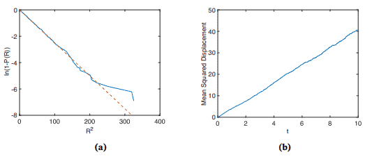
It may be that one is interested in following a single diffusing object. To do this, we make use of a fact about Brownian motion (which is the name for this process). Suppose one were able to precisely follow a particle and collect large amounts of data on its change of position, denoted $d x$, in a fixed time increment $d t$. Recall from above that the solution of the diffusion equation has the feature that the expected value of position of a particle is unchanging in time while the variance of position grows linearly in time with rate $2 D$. What this means for a fixed (small) time increment $d t$ is that $d x$ is random but distributed according to
$$
d x=\sqrt{2 D d t} \mathcal{N}(0,1) .
$$
In other words, $d x$ is a continuous random variable that is normally distributed with mean zero and variance 2 Ddt. The equation (4.1) is is called a stochastic differential equation as it specifies the change of position of the particle as a stochastic process, not as a deterministic process.
This, then, gives a formula for how to simulate a diffusion process. Specifically, let the position of the particle after $n$ time steps be denoted by $x_{n}$. Then, $x_{n}$ is updated by the formula
$$
x_{n+1}=x_{n}+d x_{n},
$$
where $d x_{n}$ is a random number chosen according to (4.1). The Matlab code that carries this out is entitled single_particle_diffusion.m, and ten examples of sample paths for a diffusing particle are shown in Figure 4.1.
数学代写|微分方程代写differential equation代考|Other Features of Brownian Particle Motion
Now that we know a little bit about how a diffusing particle moves, we can ask several other interesting questions. The first is to determine escape times. The question is as follows: How long, on average, does it take for a diffusing particle to escape from some region? In biological terms, how long does it take, on average, for a molecule that is made in the nucleus of a cell to diffuse to the boundary of the cell? Or, how long does it take a signaling molecule that is produced at the boundary of a cell to diffuse to the nucleus? A second question is, if there are two different places that a particle can escape from a region, what are the probabilities of escape through each exit? (This is called the splitting probability.)
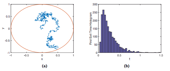
Let’s begin by simulating this. First, for the exit time problem, simulate (using Matlab code first_exit_times.m) the motion of a Brownian particle on a one-dimensional line that starts at some position $0<x<L$, and let the simulation run until the particle hits $x=L$, with the additional restriction that the particle reflects off the boundary at $x=0$, i.e., the particle position is never allowed to be negative. For obvious reasons, the boundary at $x=0$ is called a reflecting boundary and the boundary at $x=L$ is called an absorbing boundary.
An example of a simulation result is shown in Figure $4.2$, where several sample particle trajectories (a) and a histogram of first exit times for a simulation with 1,000 particles (b) are shown, with $D=1$ and $L=1$. In Figure $4.3$ are shown the simulated mean first exit times plotted as a function of initial position.
To simulate the splitting probability, start the particle at some position between $x=0$ and $x=L$ and allow the simulation to run until either $x \geq L$ or $x \leq 0$ and record the fraction of time the simulation terminates with $x \geq L$, call this $\pi_{L}$. A plot of the result from a simulation using Matlab code splitting_probability.m is shown in Figure 4.4.
数学代写|微分方程代写differential equation代考|Following Several Particles
It is possible to follow a small number of particles using the above simulation method. However, it is definitely not possible if the particle numbers are large, say a mole. To follow the diffusion of a medium number (whatever that means) of particles, we adopt the model (3.4) and do a stochastic simulation of it.
The direct stochastic simulation of (3.4) can be done using the Gillespie algorithm. To describe this algorithm, we start with the simple example of exponential decay, modeled by the equation
$$
\frac{d u}{d t}=-\alpha u .
$$
Since we already know how to track the number of particles in a single compartment, we can think about multiple compartments. Suppose there are a total of $M$ particles that are distributed among $N$ boxes, arranged in a row. Let $u_{j}, j=1, \ldots, N$, represent the integer number of particles in box $j$. We assume that each particle can leave its box and move to one of its nearest neighbors by an exponential process with rate $2 \alpha$ if it is an interior box, and rate $\alpha$ if it is a boundary box. Consequently, the rate of reaction, where by reaction we mean leaving its box, is $r_{j}=2 \alpha u_{j}$ for $j=2, \ldots, N-1$, and $r_{j}=\alpha u_{j}$ for $j=1, N$. Now, pick three uniformly distributed random numbers between 0 and 1 ; the first, $R_{1}$, we use to determine when the next reaction occurs, and the second two, $R_{2}$ and $R_{3}$, we use to determine which of the possible reactions it is. As described in Chapter 1 , the time increment to the $n$th reaction, $\delta t_{n}$, is taken to he
$$
\delta t_{n}=\frac{-1}{R_{\Sigma}} \ln R_{1},
$$
where $R_{\Sigma}=\sum_{j=1}^{K} r_{j}$. Then, take $j$ to be the smallest integer for which $R_{2}<\rho_{j}=$ $\frac{1}{R_{\Sigma}} \sum_{i=1}^{j} r_{i}$, and if $2 \leq j \leq N-1$, take the particle in the $j$ th box to move to the right if $R_{3}>\frac{1}{2}$ and to the left if $R_{3} \leq \frac{1}{2}$. If $j=1$, the particle moves to the right, and if $j=N$ it moves to the left.
Matlab code to simulate this process is titled discrete_diffusion_via_Gillespie.m. One thing worth noting is that the process becomes less and less noisy, and much slower to simulate, as more particles are included in the system, suggesting that for a sufficiently large number of particles we need not (and should not) use a Gillespie algorithm, but rather a direct simulation of the diffusion equation.
微分方程代考
数学代写|微分方程代写differential equation代考|Following Individual Particles
可能有人对跟踪单个漫射对象感兴趣。为此,我们利用了一个关于布朗运动的事实(这是这个过程的名称)。假设一个人能够精确地跟踪一个粒子并收集大量关于其位置变化的数据,表示为dX, 以固定的时间增量d吨. 回想一下,扩散方程的解具有粒子位置的期望值随时间不变而位置的方差随时间线性增长的特点。2D. 这对于固定(小)时间增量意味着什么d吨就是它dX是随机的,但根据
dX=2Dd吨ñ(0,1).
换句话说,dX是一个连续随机变量,正态分布,均值为 0,方差为 2 Ddt。方程(4.1)被称为随机微分方程,因为它将粒子位置的变化指定为随机过程,而不是确定性过程。
然后,这给出了如何模拟扩散过程的公式。具体来说,让粒子的位置在n时间步长表示为Xn. 然后,Xn由公式更新
Xn+1=Xn+dXn,
在哪里dXn是根据 (4.1) 选择的随机数。执行此操作的 Matlab 代码名为 single_particle_diffusion.m,图 4.1 显示了扩散粒子的十个样本路径示例。
数学代写|微分方程代写differential equation代考|Other Features of Brownian Particle Motion
既然我们对漫射粒子的运动方式有了一些了解,我们可以问其他几个有趣的问题。首先是确定逃生时间。问题如下:平均而言,扩散粒子从某个区域逸出需要多长时间?用生物学术语来说,在细胞核中制造的分子平均需要多长时间才能扩散到细胞边界?或者,在细胞边界产生的信号分子需要多长时间才能扩散到细胞核?第二个问题是,如果一个粒子可以从一个区域逃逸到两个不同的地方,那么通过每个出口逃逸的概率是多少?(这称为分裂概率。)
让我们从模拟这个开始。首先,对于退出时间问题,模拟(使用 Matlab 代码 first_exit_times.m)布朗粒子在从某个位置开始的一维线上的运动0<X<大号,并让模拟运行直到粒子击中X=大号, 附加限制是粒子在边界处反射X=0,即永远不允许粒子位置为负。由于显而易见的原因,边界在X=0被称为反射边界和边界在X=大号称为吸收边界。
一个模拟结果的例子如图所示4.2,其中显示了具有 1,000 个粒子的模拟的几个样本粒子轨迹 (a) 和第一次退出时间的直方图 (b),其中D=1和大号=1. 如图4.3显示了作为初始位置函数绘制的模拟平均首次退出时间。
为了模拟分裂概率,在两个之间的某个位置开始粒子X=0和X=大号并允许模拟运行直到X≥大号或者X≤0并记录模拟终止的时间分数X≥大号, 称之为圆周率大号. 图 4.4 显示了使用 Matlab 代码 split_probability.m 模拟的结果图。
数学代写|微分方程代写differential equation代考|Following Several Particles
使用上述模拟方法可以跟踪少量粒子。但是,如果粒子数很大,比如一摩尔,那肯定是不可能的。为了跟踪中等数量(无论这意味着什么)粒子的扩散,我们采用模型(3.4)并对其进行随机模拟。
(3.4) 的直接随机模拟可以使用 Gillespie 算法来完成。为了描述这个算法,我们从指数衰减的简单例子开始,由方程建模
d在d吨=−一个在.
由于我们已经知道如何跟踪单个隔间中的粒子数量,我们可以考虑多个隔间。假设总共有米分布于其中的粒子ñ盒子,排成一排。让在j,j=1,…,ñ, 表示框内粒子的整数个数j. 我们假设每个粒子可以离开它的盒子并通过指数过程移动到它的最近邻居之一,速率为2一个如果是内箱,则打分一个如果它是一个边界框。因此,反应速率,我们所说的反应是指离开它的盒子,是rj=2一个在j为了j=2,…,ñ−1, 和rj=一个在j为了j=1,ñ. 现在,在 0 和 1 之间选择三个均匀分布的随机数;首先,R1,我们用来确定下一个反应何时发生,以及后两个,R2和R3,我们用来确定它是哪些可能的反应。如第 1 章所述,时间增量为n反应,d吨n, 被带到他
d吨n=−1RΣlnR1,
在哪里RΣ=∑j=1ķrj. 然后,取j是最小的整数R2<ρj= 1RΣ∑一世=1jr一世, 而如果2≤j≤ñ−1, 取粒子jth 框向右移动 ifR3>12如果在左边R3≤12. 如果j=1,粒子向右移动,如果j=ñ它向左移动。
用于模拟此过程的 Matlab 代码名为discrete_diffusion_via_Gillespie.m。值得注意的一点是,随着系统中包含更多粒子,该过程变得越来越少,模拟速度也越来越慢,这表明对于足够多的粒子,我们不需要(也不应该)使用 Gillespie 算法,而是直接模拟扩散方程。

统计代写请认准statistics-lab™. statistics-lab™为您的留学生涯保驾护航。
金融工程代写
金融工程是使用数学技术来解决金融问题。金融工程使用计算机科学、统计学、经济学和应用数学领域的工具和知识来解决当前的金融问题,以及设计新的和创新的金融产品。
非参数统计代写
非参数统计指的是一种统计方法,其中不假设数据来自于由少数参数决定的规定模型;这种模型的例子包括正态分布模型和线性回归模型。
广义线性模型代考
广义线性模型(GLM)归属统计学领域,是一种应用灵活的线性回归模型。该模型允许因变量的偏差分布有除了正态分布之外的其它分布。
术语 广义线性模型(GLM)通常是指给定连续和/或分类预测因素的连续响应变量的常规线性回归模型。它包括多元线性回归,以及方差分析和方差分析(仅含固定效应)。
有限元方法代写
有限元方法(FEM)是一种流行的方法,用于数值解决工程和数学建模中出现的微分方程。典型的问题领域包括结构分析、传热、流体流动、质量运输和电磁势等传统领域。
有限元是一种通用的数值方法,用于解决两个或三个空间变量的偏微分方程(即一些边界值问题)。为了解决一个问题,有限元将一个大系统细分为更小、更简单的部分,称为有限元。这是通过在空间维度上的特定空间离散化来实现的,它是通过构建对象的网格来实现的:用于求解的数值域,它有有限数量的点。边界值问题的有限元方法表述最终导致一个代数方程组。该方法在域上对未知函数进行逼近。[1] 然后将模拟这些有限元的简单方程组合成一个更大的方程系统,以模拟整个问题。然后,有限元通过变化微积分使相关的误差函数最小化来逼近一个解决方案。
tatistics-lab作为专业的留学生服务机构,多年来已为美国、英国、加拿大、澳洲等留学热门地的学生提供专业的学术服务,包括但不限于Essay代写,Assignment代写,Dissertation代写,Report代写,小组作业代写,Proposal代写,Paper代写,Presentation代写,计算机作业代写,论文修改和润色,网课代做,exam代考等等。写作范围涵盖高中,本科,研究生等海外留学全阶段,辐射金融,经济学,会计学,审计学,管理学等全球99%专业科目。写作团队既有专业英语母语作者,也有海外名校硕博留学生,每位写作老师都拥有过硬的语言能力,专业的学科背景和学术写作经验。我们承诺100%原创,100%专业,100%准时,100%满意。
随机分析代写
随机微积分是数学的一个分支,对随机过程进行操作。它允许为随机过程的积分定义一个关于随机过程的一致的积分理论。这个领域是由日本数学家伊藤清在第二次世界大战期间创建并开始的。
时间序列分析代写
随机过程,是依赖于参数的一组随机变量的全体,参数通常是时间。 随机变量是随机现象的数量表现,其时间序列是一组按照时间发生先后顺序进行排列的数据点序列。通常一组时间序列的时间间隔为一恒定值(如1秒,5分钟,12小时,7天,1年),因此时间序列可以作为离散时间数据进行分析处理。研究时间序列数据的意义在于现实中,往往需要研究某个事物其随时间发展变化的规律。这就需要通过研究该事物过去发展的历史记录,以得到其自身发展的规律。
回归分析代写
多元回归分析渐进(Multiple Regression Analysis Asymptotics)属于计量经济学领域,主要是一种数学上的统计分析方法,可以分析复杂情况下各影响因素的数学关系,在自然科学、社会和经济学等多个领域内应用广泛。
MATLAB代写
MATLAB 是一种用于技术计算的高性能语言。它将计算、可视化和编程集成在一个易于使用的环境中,其中问题和解决方案以熟悉的数学符号表示。典型用途包括:数学和计算算法开发建模、仿真和原型制作数据分析、探索和可视化科学和工程图形应用程序开发,包括图形用户界面构建MATLAB 是一个交互式系统,其基本数据元素是一个不需要维度的数组。这使您可以解决许多技术计算问题,尤其是那些具有矩阵和向量公式的问题,而只需用 C 或 Fortran 等标量非交互式语言编写程序所需的时间的一小部分。MATLAB 名称代表矩阵实验室。MATLAB 最初的编写目的是提供对由 LINPACK 和 EISPACK 项目开发的矩阵软件的轻松访问,这两个项目共同代表了矩阵计算软件的最新技术。MATLAB 经过多年的发展,得到了许多用户的投入。在大学环境中,它是数学、工程和科学入门和高级课程的标准教学工具。在工业领域,MATLAB 是高效研究、开发和分析的首选工具。MATLAB 具有一系列称为工具箱的特定于应用程序的解决方案。对于大多数 MATLAB 用户来说非常重要,工具箱允许您学习和应用专业技术。工具箱是 MATLAB 函数(M 文件)的综合集合,可扩展 MATLAB 环境以解决特定类别的问题。可用工具箱的领域包括信号处理、控制系统、神经网络、模糊逻辑、小波、仿真等。