如果你也在 怎样代写数论number theory这个学科遇到相关的难题,请随时右上角联系我们的24/7代写客服。
数论是纯数学的一个分支,主要致力于研究整数和整数值函数。数论是对正整数集合的研究。
statistics-lab™ 为您的留学生涯保驾护航 在代写数论number theory方面已经树立了自己的口碑, 保证靠谱, 高质且原创的统计Statistics代写服务。我们的专家在代写数论number theory代写方面经验极为丰富,各种代写数论number theory相关的作业也就用不着说。
我们提供的数论number theory及其相关学科的代写,服务范围广, 其中包括但不限于:
- Statistical Inference 统计推断
- Statistical Computing 统计计算
- Advanced Probability Theory 高等概率论
- Advanced Mathematical Statistics 高等数理统计学
- (Generalized) Linear Models 广义线性模型
- Statistical Machine Learning 统计机器学习
- Longitudinal Data Analysis 纵向数据分析
- Foundations of Data Science 数据科学基础
数学代写|数论作业代写number theory代考|Estimates on the Growth of the Total Asymptotic Density
The study of the limit law as $m \rightarrow \infty$ for the maximal leading parameter $\mathcal{K}{\max }^{[m]}$ is a more difficult problem. This parameter is connected with the total asymptotic density of resonances $\operatorname{Ad}\left(H{\Upsilon[m]}\right)$ and so, due to Theorem 3.1, with the size $V\left(\Upsilon^{[m]}\right)$ of the random set $\Upsilon_{m}^{[m]}$. A simple version of this connection is given by the inequality $\mathcal{K}_{\max }^{[m]} \geq \frac{m}{V\left(\Upsilon^{[m]}\right)}$ a.s. (see Corollary $5.1$ (iii)). A more precise dependence in the deterministic case can be seen from [7, formula (3.6)].
The following theorem describes the rate of growth as $m \rightarrow \infty$ of the total asymptotic densities $\operatorname{Ad}\left(H_{\Upsilon[m]}\right)$ and of the sizes $V\left(\Upsilon^{[m]}\right)$, which according to Theorem $3.1$ are connected by $\operatorname{Ad}\left(H_{\left.\Upsilon^{[m]}\right]}\right)=\frac{V\left(\Upsilon^{[m]}\right)}{\pi}$ a.s.
Theorem $5.3$ Let $r>0$ and $\Upsilon^{[m]} \in \Theta\left(m, \mathbb{B}{r}\right), m \in \mathbb{N}$. Then, for any $t \in \mathbb{R}$, $$ \liminf {m \rightarrow \infty} \mathbb{P}\left{\frac{V\left(\Upsilon^{[m]}\right)}{r}>\frac{36}{35} m+\frac{2 \sqrt{87}}{35} t \sqrt{m}\right} \geq 1-\Phi(t)
$$
where $\Phi(t)=(2 \pi)^{-1 / 2} \int_{-\infty}^{t} e^{-s^{2} / 2} \mathrm{~d}$ s (the standard normal distribution function). In particular, the following estimate is valid for the asymptotic density $\operatorname{Ad}\left(H_{\Upsilon[m]}\right)$ of resonances
$$
\lim {m \rightarrow \infty} \mathbb{P}\left{\operatorname{Ad}\left(H{\Upsilon(m \mid)}\right)>\frac{m r}{\pi}\right} \rightarrow 1 \text { as } m \rightarrow \infty
$$
Proof For convenience of the notation, we replace each process $\Upsilon^{[m]}$ by the process $\widetilde{\Upsilon}^{[m]}=\left{\xi_{j}\right}_{j=1}^{m}$ defined in (5.1). This does not influence the estimates below.
Let
$m_{}=2\lfloor m / 2\rfloor$, i.e., $m_{}=m$ if $m$ is even, and $m_{}=m-1$ if $m$ is odd. Then, from the definition of $V(\cdot)$, we have $$ V\left(\widetilde{\Upsilon}^{[m]}\right) \geq 2 \mathcal{S}{m{} / 2}, \quad \text { where } \mathcal{S}{m}=\sum{j=1}^{m}\left|\xi_{2 j-1}-\xi_{2 j}\right|
$$
The $\mathbb{R}{+}$-valned random variahles $\lambda{j}:=\frac{\left|\xi_{2 j-1}-\xi_{2 j}\right|}{2 r}$ are i.i.d. with the first two moments given by
$\mathbb{E}\left(\lambda_{1}\right)=18 / 35, \quad \mathbb{E}\left(\lambda_{1}^{2}\right)=3 / 10 \quad$ (see [31] for the general formula).
Hence, the variance of $\lambda_{j}$ is $\operatorname{Var} \lambda_{j}=\left(\frac{\sqrt{87}}{35 \sqrt{2}}\right)^{2}$. Applying the Central Limit Theorem, we get
$$
\mathbb{P}\left{\frac{\mathcal{S}_{m}}{2 r}-\frac{18}{35} m \leq t \sqrt{m} \frac{\sqrt{87}}{35 \sqrt{2}}\right} \rightarrow \Phi(t)
$$
as $m \rightarrow \infty$. This implies $(5.4)$ and, in turn, (5.5)
Acknowledgements IK is grateful to Richard Froese for inspiring and educative discussions about resonances and random spectral theory, to Jürgen Prestin for the hospitality of the University of Lübeck, to Baris Evren Ugurcan and the Hausdorff Research Institute for Mathematics (HIM) of the University of Bonn for their hospitality during the trimester program “Randomness, PDEs and Nonlinear Fluctuations” at HIM in 2020. IK was supported by the VolkswagenStiftung project “Modeling, Analysis, and Approximation Theory toward applications in tomography and inverse problems” and, during the workshop “Analytical Modeling and Approximation Methods” (Berlin, 04-08.03.2020), by the VolkswagenStiftung project “From Modeling and Analysis to Approximation”.
数学代写|数论作业代写number theory代考|Green’s Functions and Euler’s Formula
An astute student in a sophomore differential equations course can compute the set of eigenvalues of the Dirichlet boundary value problem
$$
-\Delta_{D} f=-f^{\prime \prime}, \quad f(0)=f(1)=0
$$
Indeed, the underlying linear operator $-\Delta_{D}$ is the positive, self-adjoint operator in the Hilbert space $L^{2}((0,1) ; d x)$,
$$
\begin{gathered}
\left(-\Delta_{D} f\right)(x)=-f^{\prime \prime}(x) \text { for a.e. } x \in(0,1), \
f \in \operatorname{dom}\left(-\Delta_{D}\right)=\left{g \in L^{2}((0,1) ; d x) \mid g, g^{\prime} \in A C([0,1]) ; g(0)=g(1)=0\right. \
\left.g^{\prime \prime} \in L^{2}((0,1) ; d x)\right}
\end{gathered}
$$
$(A C([0,1])$ denotes the set of absolutely continuous functions on $[0,1])$, with purely discrete spectrum,
$$
\sigma\left(-\Delta_{D}\right)=\left{\lambda_{k}=(k \pi)^{2}\right}_{k \in \mathbb{N}^{*}}
$$
The eigenspace of each $\lambda_{k}$ is one-dimensional and spanned by the normalized eigenfunctions
$$
\begin{array}{ll}
-\Delta_{D} u_{k}=(k \pi)^{2} u_{k}, & u_{k}(x)=2^{1 / 2} \sin (k \pi x), 0 \leq x \leq 1 \
\left|u_{k}\right|_{\left.L^{2}((0,1) ; d x)\right)}=1, & k \in \mathbb{N}
\end{array}
$$
In particular, the collection $\left{2^{1 / 2} \sin (k \pi x)\right}_{k \in \mathbb{N}}$ forms a complete orthonormal basis in $L^{2}((0,1) ; d x)$. Since $0 \notin \sigma\left(-\Delta_{D}\right),\left(-\Delta_{D}\right)^{-1}$ exists and is explicitly given by
$$
\left(\left(-\Delta_{D}\right)^{-1} f\right)(x)=\int_{0}^{1} d y K_{1}(x, y) f(y), \quad f \in L^{2}((0,1) ; d x)
$$
where $K_{1}(\cdot, \cdot)$ denotes the Green’s function for $-\Delta_{D}$ given by
$$
K_{1}(x, y)= \begin{cases}x(1-y), & 0 \leq x \leq y \leq 1 \ y(1-x), & 0 \leq y<x \leq 1\end{cases}
$$
This operator $\left(-\Delta_{D}\right)^{-1}$ is a bounded, self-adjoint, compact operator with eigenvalues $\left{\lambda_{k}^{-1}\right}_{k=1}^{\infty}$ and associated eigenfunctions $\left{u_{k}\right}_{k=1}^{\infty}$. Moreover, as discussed below, $\left(-\Delta_{D}\right)^{-1}$ is a trace class operator and this implies
$$
\sum_{k \in \mathbb{N}} \lambda_{k}^{-1}=\int_{0}^{1} d x K_{1}(x, x)=\frac{1}{6}
$$
from which the solution to the famous “Basel problem” quickly emerges:
$$
\sum_{k \in \mathbb{N}} \frac{1}{k^{2}}=\frac{\pi^{2}}{6} .
$$
数学代写|数论作业代写number theory代考|Bernoulli Polynomials and Bernoulli Numbers
For properties of Bernoulli polynomials and Bernoulli numbers, we refer the reader to the standard sources [1] [Chap. 23] and [27] [Sects. 9.6 and 9.7] as well as the online Digital Library of Mathematical Functions https://dlmf.nist.gov/ and the accompanying book [46].
The Bernoulli polynomials $\left{B_{n}(x)\right}_{n \in \mathbb{N}{0}}$ can be defined through the generating function $$ \frac{z e^{x z}}{e^{z}-1}=\sum{n \in \mathbb{N}{0}} B{n}(x) \frac{z^{n}}{n !}, \quad|z|<2 \pi, x \in \mathbb{R}
$$
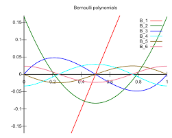
For the record, the first few Bernoulli polynomials are given by
$$
\begin{aligned}
&B_{0}(x)=1, \quad B_{1}(x)=x-\frac{1}{2}, \quad B_{2}(x)=x^{2}-x+\frac{1}{6}, \quad B_{3}(x)=x^{3}-\frac{3}{2} x^{2}+\frac{1}{2} x, \
&B_{4}(x)=x^{4}-2 x^{3}+x^{2}-\frac{1}{30}, \text { etc. }
\end{aligned}
$$
Among several properties that these polynomials satisfy, we will make use of the fact that
$$
\int_{0}^{1} d x B_{2 n}(x)=0, \quad n \geq 1
$$
which follows from the identities (see [1][23.1.8 and 23.1.11])
Green’s Functions and Euler’s Formula for $\zeta(2 n)$
33
$$
B_{n}(1-x)=(-1)^{n} B_{n}(x), \quad n \geq 1,
$$
and
$$
\int_{0}^{x} d u B_{n}(u)=\frac{B_{n+1}(x)-B_{n+1}(0)}{n+1}, \quad n \geq 1 .
$$
We also recall the Fourier cosine series expansion of $B_{2 n}(x)$ (see [1] [23.1.18] or [4] [Theorem 12.19]), which is given by
$$
\frac{(-1)^{n-1}(2 n) !}{2^{2 n-1} \pi^{2 n}} \sum_{k \in \mathbb{N}} \frac{\cos (2 k \pi x)}{k^{2 n}}=B_{2 n}(x), \quad 0 \leq x \leq 1, n \in \mathbb{N}
$$
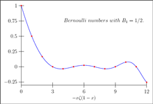
The Bernoulli numbers $\left{B_{n}\right}_{n \in \mathbb{N}{0}}$ are defined as $B{n}=B_{n}(0)$. For example,
$$
\begin{aligned}
&B_{0}=1, B_{1}=-1 / 2, B_{2}=1 / 6, B_{4}=-1 / 30, B_{6}=1 / 42, B_{8}=-1 / 30 \
&B_{10}=5 / 66, \text { etc., } B_{2 n+1}=0 \text { for } n \geq 1
\end{aligned}
$$
We will see in Sect. 4 , that the Green’s function $K_{n}(\cdot, \cdot)$, associated with the $n^{t h}$ power of the operator $-\Delta_{D}$ defined in (1.1), can be given explicitly in terms of Bernoulli polynomials.
数论作业代写
数学代写|数论作业代写number theory代考|Estimates on the Growth of the Total Asymptotic Density
极限律的研究米→∞对于最大前导参数ķ最大限度[米]是一个比较困难的问题。该参数与共振的总渐近密度有关广告(HΥ[米])因此,由于定理 3.1,大小在(Υ[米])随机集的Υ米[米]. 这种连接的一个简单版本由不等式给出ķ最大限度[米]≥米在(Υ[米])如(见推论5.1(iii))。从[7,公式(3.6)]可以看出确定性情况下更精确的依赖关系。
以下定理将增长率描述为米→∞总渐近密度的广告(HΥ[米])和尺寸在(Υ[米]), 根据定理3.1由广告(HΥ[米]])=在(Υ[米])圆周率作为
定理5.3让r>0和Υ[米]∈θ(米,乙r),米∈ñ. 那么,对于任何吨∈R,
\liminf {m \rightarrow \infty} \mathbb{P}\left{\frac{V\left(\Upsilon^{[m]}\right)}{r}>\frac{36}{35} m+\ frac{2 \sqrt{87}}{35} t \sqrt{m}\right} \geq 1-\Phi(t)\liminf {m \rightarrow \infty} \mathbb{P}\left{\frac{V\left(\Upsilon^{[m]}\right)}{r}>\frac{36}{35} m+\ frac{2 \sqrt{87}}{35} t \sqrt{m}\right} \geq 1-\Phi(t)
在哪里披(吨)=(2圆周率)−1/2∫−∞吨和−s2/2 ds(标准正态分布函数)。特别是,以下估计对渐近密度有效广告(HΥ[米])共振
\lim {m \rightarrow \infty} \mathbb{P}\left{\operatorname{Ad}\left(H{\Upsilon(m \mid)}\right)>\frac{m r}{\pi}\right } \rightarrow 1 \text { as } m \rightarrow \infty\lim {m \rightarrow \infty} \mathbb{P}\left{\operatorname{Ad}\left(H{\Upsilon(m \mid)}\right)>\frac{m r}{\pi}\right } \rightarrow 1 \text { as } m \rightarrow \infty
证明 为了记号方便,我们替换每个过程Υ[米]通过过程\widetilde{\Upsilon}^{[m]}=\left{\xi_{j}\right}_{j=1}^{m}\widetilde{\Upsilon}^{[m]}=\left{\xi_{j}\right}_{j=1}^{m}在 (5.1) 中定义。这不影响下面的估计。
让
米=2⌊米/2⌋, IE,米=米如果米是偶数,并且米=米−1如果米很奇怪。那么,从定义在(⋅), 我们有
在(Υ~[米])≥2小号米/2, 在哪里 小号米=∑j=1米|X2j−1−X2j|
这R+-valned 随机变量λj:=|X2j−1−X2j|2r与前两个时刻是独立同分布的
和(λ1)=18/35,和(λ12)=3/10(通式见[31])。
因此,方差λj是曾是λj=(87352)2. 应用中心极限定理,我们得到
\mathbb{P}\left{\frac{\mathcal{S}_{m}}{2 r}-\frac{18}{35} m \leq t \sqrt{m} \frac{\sqrt{87 }}{35 \sqrt{2}}\right} \rightarrow \Phi(t)\mathbb{P}\left{\frac{\mathcal{S}_{m}}{2 r}-\frac{18}{35} m \leq t \sqrt{m} \frac{\sqrt{87 }}{35 \sqrt{2}}\right} \rightarrow \Phi(t)
作为米→∞. 这意味着(5.4)(5.5)
致谢 IK 感谢 Richard Froese 关于共振和随机光谱理论的启发性和教育性讨论,感谢 Jürgen Prestin 对吕贝克大学的热情款待,感谢 Baris Evren Ugurcan 和 Hausdorff 数学研究所波恩大学 (HIM) 于 2020 年在 HIM 的三个月计划“随机性、偏微分方程和非线性波动”期间热情好客。IK 得到了大众汽车基金会项目“建模、分析和近似理论在断层扫描和逆问题中的应用的支持” ”,并且在“分析建模和近似方法”研讨会(柏林,04-08.03.2020)期间,由大众汽车基金会项目“从建模和分析到近似”。
数学代写|数论作业代写number theory代考|Green’s Functions and Euler’s Formula
学习二年级微分方程课程的机敏学生可以计算狄利克雷边值问题的特征值集
−ΔDF=−F′′,F(0)=F(1)=0
实际上,底层的线性算子−ΔD是希尔伯特空间中的正自伴算子大号2((0,1);dX),
\begin{聚集} \left(-\Delta_{D} f\right)(x)=-f^{\prime \prime}(x) \text { for ae } x \in(0,1), \ f \in \operatorname{dom}\left(-\Delta_{D}\right)=\left{g \in L^{2}((0,1) ; d x) \mid g, g^{\prime } \in A C([0,1]) ; g(0)=g(1)=0\对。\ \left.g^{\prime \prime} \in L^{2}((0,1) ; d x)\right} \end{聚集}\begin{聚集} \left(-\Delta_{D} f\right)(x)=-f^{\prime \prime}(x) \text { for ae } x \in(0,1), \ f \in \operatorname{dom}\left(-\Delta_{D}\right)=\left{g \in L^{2}((0,1) ; d x) \mid g, g^{\prime } \in A C([0,1]) ; g(0)=g(1)=0\对。\ \left.g^{\prime \prime} \in L^{2}((0,1) ; d x)\right} \end{聚集}
(一种C([0,1])表示绝对连续函数的集合[0,1]),具有纯离散谱,
\sigma\left(-\Delta_{D}\right)=\left{\lambda_{k}=(k \pi)^{2}\right}_{k \in \mathbb{N}^{*} }\sigma\left(-\Delta_{D}\right)=\left{\lambda_{k}=(k \pi)^{2}\right}_{k \in \mathbb{N}^{*} }
每个的特征空间λķ是一维的,由归一化的特征函数跨越
−ΔD在ķ=(ķ圆周率)2在ķ,在ķ(X)=21/2罪(ķ圆周率X),0≤X≤1 |在ķ|大号2((0,1);dX))=1,ķ∈ñ
特别是,该系列\left{2^{1 / 2} \sin (k \pi x)\right}_{k \in \mathbb{N}}\left{2^{1 / 2} \sin (k \pi x)\right}_{k \in \mathbb{N}}形成一个完整的正交基大号2((0,1);dX). 自从0∉σ(−ΔD),(−ΔD)−1存在并且由下式明确给出
((−ΔD)−1F)(X)=∫01d是ķ1(X,是)F(是),F∈大号2((0,1);dX)
在哪里ķ1(⋅,⋅)表示格林函数−ΔD由
ķ1(X,是)={X(1−是),0≤X≤是≤1 是(1−X),0≤是<X≤1
该运算符(−ΔD)−1是具有特征值的有界、自伴、紧算子\left{\lambda_{k}^{-1}\right}_{k=1}^{\infty}\left{\lambda_{k}^{-1}\right}_{k=1}^{\infty}和相关的特征函数\left{u_{k}\right}_{k=1}^{\infty}\left{u_{k}\right}_{k=1}^{\infty}. 此外,如下所述,(−ΔD)−1是一个跟踪类运算符,这意味着
∑ķ∈ñλķ−1=∫01dXķ1(X,X)=16
著名的“巴塞尔问题”的解决方案很快就出现了:
∑ķ∈ñ1ķ2=圆周率26.
数学代写|数论作业代写number theory代考|Bernoulli Polynomials and Bernoulli Numbers
对于伯努利多项式和伯努利数的性质,我们建议读者参考标准资料 [1] [Chap. 23] 和 [27] [教派。9.6 和 9.7] 以及在线数学函数数字图书馆 https://dlmf.nist.gov/ 和随附的书 [46]。
伯努利多项式\left{B_{n}(x)\right}_{n \in \mathbb{N}{0}}\left{B_{n}(x)\right}_{n \in \mathbb{N}{0}}可以通过生成函数定义
和和X和和和−1=∑n∈ñ0乙n(X)和nn!,|和|<2圆周率,X∈R
作为记录,前几个伯努利多项式由下式给出
乙0(X)=1,乙1(X)=X−12,乙2(X)=X2−X+16,乙3(X)=X3−32X2+12X, 乙4(X)=X4−2X3+X2−130, 等等
在这些多项式满足的几个性质中,我们将利用以下事实:
∫01dX乙2n(X)=0,n≥1
它来自身份(参见 [1] [23.1.8 和 23.1.11])
格林函数和欧拉公式G(2n)
33
乙n(1−X)=(−1)n乙n(X),n≥1,
和
∫0Xd在乙n(在)=乙n+1(X)−乙n+1(0)n+1,n≥1.
我们还记得傅里叶余弦级数展开乙2n(X)(参见 [1] [23.1.18] 或 [4] [定理 12.19]),由下式给出
(−1)n−1(2n)!22n−1圆周率2n∑ķ∈ñ因(2ķ圆周率X)ķ2n=乙2n(X),0≤X≤1,n∈ñ
伯努利数 $\left{B_{n}\right}_{n \in \mathbb{N} {0}}一个r和d和F一世n和d一个sB {n}=B_{n}(0).F○r和X一个米pl和,乙0=1,乙1=−1/2,乙2=1/6,乙4=−1/30,乙6=1/42,乙8=−1/30 乙10=5/66, ETC。, 乙2n+1=0 为了 n≥1在和在一世lls和和一世n小号和C吨.4,吨H一个吨吨H和Gr和和n′sF在nC吨一世○nK_{n}(\cdot, \cdot),一个ss○C一世一个吨和d在一世吨H吨H和n^{第}p○在和r○F吨H和○p和r一个吨○r-\Delta_{D}$ 在 (1.1) 中定义,可以根据伯努利多项式明确给出。

统计代写请认准statistics-lab™. statistics-lab™为您的留学生涯保驾护航。
金融工程代写
金融工程是使用数学技术来解决金融问题。金融工程使用计算机科学、统计学、经济学和应用数学领域的工具和知识来解决当前的金融问题,以及设计新的和创新的金融产品。
非参数统计代写
非参数统计指的是一种统计方法,其中不假设数据来自于由少数参数决定的规定模型;这种模型的例子包括正态分布模型和线性回归模型。
广义线性模型代考
广义线性模型(GLM)归属统计学领域,是一种应用灵活的线性回归模型。该模型允许因变量的偏差分布有除了正态分布之外的其它分布。
术语 广义线性模型(GLM)通常是指给定连续和/或分类预测因素的连续响应变量的常规线性回归模型。它包括多元线性回归,以及方差分析和方差分析(仅含固定效应)。
有限元方法代写
有限元方法(FEM)是一种流行的方法,用于数值解决工程和数学建模中出现的微分方程。典型的问题领域包括结构分析、传热、流体流动、质量运输和电磁势等传统领域。
有限元是一种通用的数值方法,用于解决两个或三个空间变量的偏微分方程(即一些边界值问题)。为了解决一个问题,有限元将一个大系统细分为更小、更简单的部分,称为有限元。这是通过在空间维度上的特定空间离散化来实现的,它是通过构建对象的网格来实现的:用于求解的数值域,它有有限数量的点。边界值问题的有限元方法表述最终导致一个代数方程组。该方法在域上对未知函数进行逼近。[1] 然后将模拟这些有限元的简单方程组合成一个更大的方程系统,以模拟整个问题。然后,有限元通过变化微积分使相关的误差函数最小化来逼近一个解决方案。
tatistics-lab作为专业的留学生服务机构,多年来已为美国、英国、加拿大、澳洲等留学热门地的学生提供专业的学术服务,包括但不限于Essay代写,Assignment代写,Dissertation代写,Report代写,小组作业代写,Proposal代写,Paper代写,Presentation代写,计算机作业代写,论文修改和润色,网课代做,exam代考等等。写作范围涵盖高中,本科,研究生等海外留学全阶段,辐射金融,经济学,会计学,审计学,管理学等全球99%专业科目。写作团队既有专业英语母语作者,也有海外名校硕博留学生,每位写作老师都拥有过硬的语言能力,专业的学科背景和学术写作经验。我们承诺100%原创,100%专业,100%准时,100%满意。
随机分析代写
随机微积分是数学的一个分支,对随机过程进行操作。它允许为随机过程的积分定义一个关于随机过程的一致的积分理论。这个领域是由日本数学家伊藤清在第二次世界大战期间创建并开始的。
时间序列分析代写
随机过程,是依赖于参数的一组随机变量的全体,参数通常是时间。 随机变量是随机现象的数量表现,其时间序列是一组按照时间发生先后顺序进行排列的数据点序列。通常一组时间序列的时间间隔为一恒定值(如1秒,5分钟,12小时,7天,1年),因此时间序列可以作为离散时间数据进行分析处理。研究时间序列数据的意义在于现实中,往往需要研究某个事物其随时间发展变化的规律。这就需要通过研究该事物过去发展的历史记录,以得到其自身发展的规律。
回归分析代写
多元回归分析渐进(Multiple Regression Analysis Asymptotics)属于计量经济学领域,主要是一种数学上的统计分析方法,可以分析复杂情况下各影响因素的数学关系,在自然科学、社会和经济学等多个领域内应用广泛。
MATLAB代写
MATLAB 是一种用于技术计算的高性能语言。它将计算、可视化和编程集成在一个易于使用的环境中,其中问题和解决方案以熟悉的数学符号表示。典型用途包括:数学和计算算法开发建模、仿真和原型制作数据分析、探索和可视化科学和工程图形应用程序开发,包括图形用户界面构建MATLAB 是一个交互式系统,其基本数据元素是一个不需要维度的数组。这使您可以解决许多技术计算问题,尤其是那些具有矩阵和向量公式的问题,而只需用 C 或 Fortran 等标量非交互式语言编写程序所需的时间的一小部分。MATLAB 名称代表矩阵实验室。MATLAB 最初的编写目的是提供对由 LINPACK 和 EISPACK 项目开发的矩阵软件的轻松访问,这两个项目共同代表了矩阵计算软件的最新技术。MATLAB 经过多年的发展,得到了许多用户的投入。在大学环境中,它是数学、工程和科学入门和高级课程的标准教学工具。在工业领域,MATLAB 是高效研究、开发和分析的首选工具。MATLAB 具有一系列称为工具箱的特定于应用程序的解决方案。对于大多数 MATLAB 用户来说非常重要,工具箱允许您学习和应用专业技术。工具箱是 MATLAB 函数(M 文件)的综合集合,可扩展 MATLAB 环境以解决特定类别的问题。可用工具箱的领域包括信号处理、控制系统、神经网络、模糊逻辑、小波、仿真等。