如果你也在 怎样代写概率论Probability theory这个学科遇到相关的难题,请随时右上角联系我们的24/7代写客服。
概率论是与概率有关的数学分支。虽然有几种不同的概率解释,但概率论以严格的数学方式处理这一概念,通过一套公理来表达它。
statistics-lab™ 为您的留学生涯保驾护航 在代写概率论Probability theory方面已经树立了自己的口碑, 保证靠谱, 高质且原创的统计Statistics代写服务。我们的专家在代写概率论Probability theory代写方面经验极为丰富,各种代写概率论Probability theory相关的作业也就用不着说。
我们提供的概率论Probability theory及其相关学科的代写,服务范围广, 其中包括但不限于:
- Statistical Inference 统计推断
- Statistical Computing 统计计算
- Advanced Probability Theory 高等概率论
- Advanced Mathematical Statistics 高等数理统计学
- (Generalized) Linear Models 广义线性模型
- Statistical Machine Learning 统计机器学习
- Longitudinal Data Analysis 纵向数据分析
- Foundations of Data Science 数据科学基础
数学代写|概率论代写Probability theory代考|Adaptive MH Algorithm
The adaptive MH (AMH) algorithm was proposed by Beck and Au [22] to settle the difficulty in sampling according to the posterior PDF directly. The algorithm introduces a sequence of intermediate PDFs that converge to the posterior PDF for sample generation, and finally achieves the samples from the posterior PDF.
Let $\left{p^{(1)}, p^{(2)}, \ldots, p^{\left(s_{0}\right)}\right}$ denotes a sequence of PDFs, and $p^{(s)}$ is chosen as updated PDF from Bayes’ theorem based on an increasing amount of data:
$$
p^{(s)}=p\left(\theta \mid D^{(s)}, C\right)
$$
where $D^{(1)} \subset D^{(2)} \subset \ldots \subset D^{\left(s_{0}\right)}=D$. If the updated PDF with data $D$ has the following form:
$$
p(\theta \mid D, C)=c \exp \left(-\frac{J(\theta)}{2 \varphi^{2}}\right)
$$
where $J(\theta)$ is the goodness-of-fit function, and $\varphi$ is a measure of the size of the prediction error. Therefore, the sequence $\left{p^{(s)}\right}$ can be constructed as:
$$
p^{(s)}=c^{(s)} \exp \left(-\frac{J(\theta)}{2\left(\varphi^{(s)}\right)^{2}}\right)
$$
where $\left(\varphi^{(s)}\right)^{2}=2^{s_{0}-s} \varphi^{2}$ with $2^{s_{n}} \approx \varphi^{-2}$ if the length scale of the prior PDF is of order one. The following content shows the main steps of AMH algorithm:
(1) Starting with the prior PDF as the proposal PDF and $p^{(1)}$ as the target PDF, simulate the samples $\left{\theta_{1}^{(1)}, \theta_{2}^{(1)}, \ldots, \theta_{N}^{(1)}\right}$ by using the MH algorithm;
(2) At the sth level, simulate the samples using the procedure similar to level 1 except that the proposal PDF in MH algorithm is constructed by the kernel density. The kernel density or proposal PDF at the sth level can be constructed by using the samples generated at the $(s-1)$ th level:
$$
p^{(s-1)}(\theta)=\sum_{n-1}^{N} w_{n} g\left(\theta ; \theta_{n}^{(s-1)}, \sum_{n}\right)
$$
where $g\left(\theta ; \boldsymbol{\theta}{n}^{(s-1)}, \Sigma{n}\right)$ is the multidimensional Gaussian PDF evaluated at $\boldsymbol{\theta}$ with mean $\boldsymbol{\theta}{n}^{(s-1)}$ and covariance matrix $\Sigma{n} ; w_{n}$ is the weight with $\sum_{n=1}^{N} w_{n}=1$.
(3) Repeat step (2) until the $s_{0}$ th simulation level is finished, and obtain the samples from the target updated PDF $p(\theta \mid D, C)=p^{\left(5_{0}\right)}$.
With the help of AMH algorithm, the samples can be simulated from the posterior PDF that is very peaked or multimodal. However, this algorithm is still inefficient for the high-dimensional problems due to the inefficiency of kernel density estimations for high-dimensional problems. Based on experience, problem may arise when the number of uncertainty parameters is more than $4 .$
数学代写|概率论代写Probability theory代考|Transitional Markov Chain Monte Carlo Method
The transitional Markov chain Monte Carlo (TMCMC) method was proposed by Ching and Chen [47] on the basis of AMH algorithm. The TMCMC algorithm uses the same idea of “intermediate PDFs” as proposed by Beck and Au [22], but it does not require kernel density estimation. An additional advantage is that the intermediate PDFs can be automatically selected. The sequence of intermediate PDFs will ultimately converge to the posterior PDF and is defined by:
$$
f_{s}(\theta) \propto f(\theta \mid C) \cdot f(D \mid \theta, C)^{p_{x}}\left(s=0,1, \ldots, N_{s} ; 0=p_{0}<p_{1}<\cdots<p_{N_{x}}=1\right)
$$
where the subscript $s$ denotes the stage number and $N_{S}$ is the total number. The PDF of the initial stage with $p_{0}=0$ is proportional to the prior PDF, while the PDF of the
final stage with $p_{N_{x}}=1$ is proportional to the posterior PDF. The used intermediate PDFs can enable a good means of transitioning and obtaining the samples between the adjacent intermediate PDFs. Besides, the TMCMC algorithm can also estimate the evidence without solving any integral problem. The said algorithm can be enacted by following these steps:
(i) At the initial stage $(s=0)$, draw the samples $\left{\theta_{0, k}: k=1,2, \ldots, N_{0}\right}$ according to the prior $\operatorname{PDF} f_{0}(\theta)$;
(ii) Choose $p_{s+1}$ such that the COV of $\left{f\left(D \mid \theta_{s, k}, C\right)^{p_{s+1}-p_{s}}: k=1,2, \ldots, N_{s}\right}$ is equal to a prescribed threshold. Then, compute the plausibility weights $w\left(\boldsymbol{\theta}{s, k}\right)=f\left(D \mid \boldsymbol{\theta}{s, k}, C\right)^{p_{x+1}-p_{s}}$ for $k=1,2, \ldots, N_{s}$ and $S_{s}=\sum_{k=1}^{N_{x}} w\left(\boldsymbol{\theta}{s, k}\right) / N{s} .$ Here, $\theta_{s, k}$ denotes the $k$ th sample that belongs to level $s$ and the factor will be used to compute the evidence $f(D \mid C)$;
(iii) Apply the $\mathrm{MH}$ algorithm to generate the samples $\left{\theta_{s+1, k}: k=1,2, \ldots, N_{s+1}\right}$ from $f_{s+1}(\theta)$. The candidate sample $\boldsymbol{\theta}^{c}$ of the sth sample in the Markov chain is generated from $N\left(\theta_{s, l}, \Sigma_{s}\right)$, in which $\theta_{s, l}$ is one of the current samples $\left{\theta_{s, l}: l=1,2, \ldots, N_{s}\right}$. The lth initial sample $\boldsymbol{\theta}{s, l}$ is chosen with probability $w\left(\boldsymbol{\theta}{s, l}\right) / \sum_{l=1}^{N_{s}} w\left(\boldsymbol{\theta}{s, l}\right) . \Sigma{s}$ is the covariance matrix of the Gaussian proposal PDF centered at the current sample $\left{\theta_{s, l}: l=1,2, \ldots, N_{s}\right}$ and can be estimated using the following equation:
$$
\begin{aligned}
\sum_{s}=\beta^{2} \sum_{k=1}^{N_{s}} w\left(\boldsymbol{\theta}{s, k}\right) &\left{\boldsymbol{\theta}{s, k}-\left[\sum_{l=1}^{N_{s}} w\left(\boldsymbol{\theta}{s, l}\right) \boldsymbol{\theta}{s, l} / \sum_{l=1}^{N_{s}} w\left(\boldsymbol{\theta}{s, l}\right)\right]\right} \ & \times\left{\boldsymbol{\theta}{s, k}-\left[\sum_{l=1}^{N_{s}} w\left(\boldsymbol{\theta}{s, l}\right) \boldsymbol{\theta}{s, l} / \sum_{l=1}^{N_{s}} w\left(\boldsymbol{\theta}_{s, l}\right)\right]\right}^{T}
\end{aligned}
$$
数学代写|概率论代写Probability theory代考|Soil Suction
According to the level of the water contained in the soils, the soils can be divided into two broad categories: saturated soils and unsaturated soils. The unsaturated soil is commonly defined as having three phases: solid, water and air. However, the air-water interface or contractile skin must be considered as an independent phase when considering the stress state of unsaturated soil [48]. Since the 1930 s, the geotechnical scholars began to study the issue of unsaturated soils. The suction is an important factor for studying the properties of unsaturated soils. It exhibits the intensity of interaction between soil-water and soil particles and the curvature state of the air-water interface in unsaturated soil [48].
The total suction consists of two components: matric suction (matric or capillary component of free energy) and osmotic suction (osmotic or solute component of free energy). Aitchison [49] gave the total suction as follows:
$$
\phi=\left(u_{a}-u_{w}\right)+\pi
$$
where $\phi$ denotes total suction; $\left(u_{a}-u_{w}\right.$ ) denotes matric suction, in which $u_{a}$ and $u_{w}$ represent pore-air and pore-water pressure, respectively; and $\pi$ denotes the osmotic suction.
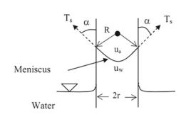
As shown in Fig. 1.1, water rises in a capillary tube immersed in water, similar to the pores of the soil with small radius acting as capillary tubes that cause the soil water to rise above the water table. The pressure of capillary water is negative relative to the air pressure, which is generally atmospheric (i.e., $u_{a}=0$ ). Therefore, the capillary pressure, that is, matric suction, can be expressed as follows:
$$
u_{a}-u_{w}=\frac{2 T_{s} \cos \alpha}{r}
$$
where $T_{s}$ is the surface tension of water; $\alpha$ is the contact angle; $r$ is the radius of the capillary tube, that is, the radius of the pore in the soil. It can be seen from Eq. (1.23) that the matric suction increases as the pore radius decreases.
Some researchers have studied the effect of suction on the shear strength, permeability and compressibility of soils. Most experimental evidences show the shear strength increases nonlinearly with soil suction, and the brittleness and dilatancy of an unsaturated soil also increase [50-53]. Fredlund and Rahardjo [54] stated that the permeability of an unsaturated soil depends on degree of saturation, and it can be estimated using the relationship between degree of saturation and suction. Alonso et al. [55] pointed that the compressibility of an unsaturated soil generally increases with the decrease of suction. Wheeler and Sivakumar [56] and Chiu and Ng [57] found that the compressibility under unsaturated conditions is larger than that under saturated conditions through the experiments. Estabragh et al. [58] found that the compressibility of a compacted silty soil does not change monotonically with suction, and it reaches maximum at certain suction. On the other hand, the osmotic suction is insensitive to the changes of soil-water content [54].
概率论代考
数学代写|概率论代写Probability theory代考|Adaptive MH Algorithm
Beck和Au [22]提出了自适应MH(AMH)算法,以解决直接根据后验PDF进行采样的困难。该算法引入了一系列中间PDF,这些中间PDF会收敛到后验PDF进行样本生成,最终从后验PDF获得样本。
让\left{p^{(1)}, p^{(2)}, \ldots, p^{\left(s_{0}\right)}\right}\left{p^{(1)}, p^{(2)}, \ldots, p^{\left(s_{0}\right)}\right}表示 PDF 序列,并且p(s)根据越来越多的数据,从贝叶斯定理中选择更新的 PDF:
p(s)=p(θ∣D(s),C)
在哪里D(1)⊂D(2)⊂…⊂D(s0)=D. 如果更新的 PDF 带有数据D具有以下形式:
p(θ∣D,C)=C经验(−Ĵ(θ)2披2)
在哪里Ĵ(θ)是拟合优度函数,并且披是预测误差大小的度量。因此,序列\left{p^{(s)}\right}\left{p^{(s)}\right}可以构造为:
p(s)=C(s)经验(−Ĵ(θ)2(披(s))2)
在哪里(披(s))2=2s0−s披2和2sn≈披−2如果先前 PDF 的长度比例是一阶的。以下内容展示了 AMH 算法的主要步骤:
(1) 从先验 PDF 作为提案 PDF 开始,p(1)作为目标PDF,模拟样本\left{\theta_{1}^{(1)}, \theta_{2}^{(1)}, \ldots, \theta_{N}^{(1)}\right}\left{\theta_{1}^{(1)}, \theta_{2}^{(1)}, \ldots, \theta_{N}^{(1)}\right}通过使用MH算法;
(2) 在第 s 层,使用类似于第 1 层的过程模拟样本,不同之处在于 MH 算法中的提议 PDF 是由核密度构造的。第s层的核密度或proposal PDF可以通过使用在第s层生成的样本来构建(s−1)级别:
p(s−1)(θ)=∑n−1ñ在nG(θ;θn(s−1),∑n)
在哪里G(θ;θn(s−1),Σn)是评估的多维高斯 PDFθ平均θn(s−1)和协方差矩阵Σn;在n是重量∑n=1ñ在n=1.
(3) 重复步骤 (2) 直到s0仿真关卡完成,从目标更新的PDF中获取样本p(θ∣D,C)=p(50).
在 AMH 算法的帮助下,可以从非常峰值或多峰的后验 PDF 中模拟样本。然而,由于核密度估计对高维问题的效率低下,该算法对于高维问题仍然效率低下。根据经验,当不确定参数的数量大于4.
数学代写|概率论代写Probability theory代考|Transitional Markov Chain Monte Carlo Method
过渡马尔可夫链蒙特卡洛(TMCMC)方法是由Ching和Chen [47]在AMH算法的基础上提出的。TMCMC 算法使用与 Beck 和 Au [22] 提出的“中间 PDF”相同的想法,但它不需要核密度估计。另一个优点是可以自动选择中间 PDF。中间 PDF 的序列最终将收敛到后验 PDF,并由下式定义:
Fs(θ)∝F(θ∣C)⋅F(D∣θ,C)pX(s=0,1,…,ñs;0=p0<p1<⋯<pñX=1)
下标在哪里s表示阶段编号和ñ小号是总数。初始阶段的PDFp0=0与先前的 PDF 成正比,而
最后阶段pñX=1与后验 PDF 成正比。使用的中间 PDF 可以很好地在相邻中间 PDF 之间转换和获取样本。此外,TMCMC 算法还可以在不解决任何积分问题的情况下估计证据。所述算法可以通过以下步骤来制定:
(i) 在初始阶段(s=0), 抽取样本\left{\theta_{0, k}: k=1,2, \ldots, N_{0}\right}\left{\theta_{0, k}: k=1,2, \ldots, N_{0}\right}根据之前的PDF格式F0(θ);
(ii) 选择ps+1这样的 COV\left{f\left(D \mid \theta_{s, k}, C\right)^{p_{s+1}-p_{s}}: k=1,2, \ldots, N_{s} \正确的}\left{f\left(D \mid \theta_{s, k}, C\right)^{p_{s+1}-p_{s}}: k=1,2, \ldots, N_{s} \正确的}等于规定的阈值。然后,计算合理性权重在(θs,ķ)=F(D∣θs,ķ,C)pX+1−ps为了ķ=1,2,…,ñs和小号s=∑ķ=1ñX在(θs,ķ)/ñs.这里,θs,ķ表示ķ属于级别的第 th 个样本s并且该因子将用于计算证据F(D∣C);
(iii) 应用米H生成样本的算法\left{\theta_{s+1, k}: k=1,2, \ldots, N_{s+1}\right}\left{\theta_{s+1, k}: k=1,2, \ldots, N_{s+1}\right}从Fs+1(θ). 候选样本θC马尔可夫链中第 s 个样本的ñ(θs,l,Σs), 其中θs,l是当前样本之一\left{\theta_{s, l}: l=1,2, \ldots, N_{s}\right}\left{\theta_{s, l}: l=1,2, \ldots, N_{s}\right}. 第 l 个初始样本θs,l被概率选中在(θs,l)/∑l=1ñs在(θs,l).Σs是以当前样本为中心的高斯提议 PDF 的协方差矩阵\left{\theta_{s, l}: l=1,2, \ldots, N_{s}\right}\left{\theta_{s, l}: l=1,2, \ldots, N_{s}\right}并且可以使用以下等式进行估计:
\begin{aligned} \sum_{s}=\beta^{2} \sum_{k=1}^{N_{s}} w\left(\boldsymbol{\theta}{s, k}\right) & \left{\boldsymbol{\theta}{s, k}-\left[\sum_{l=1}^{N_{s}} w\left(\boldsymbol{\theta}{s, l}\right) \boldsymbol{\theta}{s, l} / \sum_{l=1}^{N_{s}} w\left(\boldsymbol{\theta}{s, l}\right)\right]\right} \ & \times\left{\boldsymbol{\theta}{s, k}-\left[\sum_{l=1}^{N_{s}} w\left(\boldsymbol{\theta}{s, l }\right) \boldsymbol{\theta}{s, l} / \sum_{l=1}^{N_{s}} w\left(\boldsymbol{\theta}_{s, l}\right)\右]\right}^{T} \end{对齐}\begin{aligned} \sum_{s}=\beta^{2} \sum_{k=1}^{N_{s}} w\left(\boldsymbol{\theta}{s, k}\right) & \left{\boldsymbol{\theta}{s, k}-\left[\sum_{l=1}^{N_{s}} w\left(\boldsymbol{\theta}{s, l}\right) \boldsymbol{\theta}{s, l} / \sum_{l=1}^{N_{s}} w\left(\boldsymbol{\theta}{s, l}\right)\right]\right} \ & \times\left{\boldsymbol{\theta}{s, k}-\left[\sum_{l=1}^{N_{s}} w\left(\boldsymbol{\theta}{s, l }\right) \boldsymbol{\theta}{s, l} / \sum_{l=1}^{N_{s}} w\left(\boldsymbol{\theta}_{s, l}\right)\右]\right}^{T} \end{对齐}
数学代写|概率论代写Probability theory代考|Soil Suction
根据土壤中含水量的高低,土壤可分为两大类:饱和土壤和非饱和土壤。非饱和土通常被定义为具有三个阶段:固体、水和空气。然而,在考虑非饱和土的应力状态时,必须将气水界面或收缩表皮视为一个独立相[48]。1930年代以来,岩土学者开始研究非饱和土问题。吸力是研究非饱和土性质的重要因素。它展示了非饱和土壤中土壤-水和土壤颗粒之间相互作用的强度以及空气-水界面的曲率状态[48]。
总吸力由两部分组成:基质吸力(自由能的基质或毛细血管成分)和渗透吸力(自由能的渗透或溶质成分)。Aitchison [49] 给出的总吸力如下:
φ=(在一个−在在)+圆周率
在哪里φ表示总吸力;(在一个−在在) 表示基质吸力,其中在一个和在在分别代表孔隙空气压力和孔隙水压力;和圆周率表示渗透吸力。
如图 1.1 所示,水在浸入水中的毛细管中上升,类似于土壤的小半径孔隙充当毛细管,使土壤水上升到地下水位以上。毛细管水的压力相对于大气压力为负,大气压力通常为大气压(即,在一个=0)。因此,毛细压力,即基质吸力,可表示为:
在一个−在在=2吨s因一个r
在哪里吨s是水的表面张力;一个是接触角;r是毛细管的半径,即土壤中孔隙的半径。从方程式可以看出。(1.23) 基质吸力随着孔隙半径的减小而增加。
一些研究人员研究了吸力对土壤的剪切强度、渗透性和压缩性的影响。大多数实验证据表明,抗剪强度随土壤吸力非线性增加,非饱和土的脆性和剪胀性也增加[50-53]。Fredlund 和 Rahardjo [54] 指出,非饱和土壤的渗透性取决于饱和度,并且可以使用饱和度和吸力之间的关系来估计。阿隆索等人。[55] 指出,非饱和土的可压缩性通常随着吸力的降低而增加。Wheeler 和 Sivakumar [56] 以及 Chiu 和 Ng [57] 通过实验发现非饱和条件下的压缩率大于饱和条件下的压缩率。埃斯塔布拉等人。[58] 发现压实粉质土的压缩性不随吸力单调变化,在一定吸力下达到最大值。另一方面,渗透吸力对土壤含水量的变化不敏感[54]。

统计代写请认准statistics-lab™. statistics-lab™为您的留学生涯保驾护航。
金融工程代写
金融工程是使用数学技术来解决金融问题。金融工程使用计算机科学、统计学、经济学和应用数学领域的工具和知识来解决当前的金融问题,以及设计新的和创新的金融产品。
非参数统计代写
非参数统计指的是一种统计方法,其中不假设数据来自于由少数参数决定的规定模型;这种模型的例子包括正态分布模型和线性回归模型。
广义线性模型代考
广义线性模型(GLM)归属统计学领域,是一种应用灵活的线性回归模型。该模型允许因变量的偏差分布有除了正态分布之外的其它分布。
术语 广义线性模型(GLM)通常是指给定连续和/或分类预测因素的连续响应变量的常规线性回归模型。它包括多元线性回归,以及方差分析和方差分析(仅含固定效应)。
有限元方法代写
有限元方法(FEM)是一种流行的方法,用于数值解决工程和数学建模中出现的微分方程。典型的问题领域包括结构分析、传热、流体流动、质量运输和电磁势等传统领域。
有限元是一种通用的数值方法,用于解决两个或三个空间变量的偏微分方程(即一些边界值问题)。为了解决一个问题,有限元将一个大系统细分为更小、更简单的部分,称为有限元。这是通过在空间维度上的特定空间离散化来实现的,它是通过构建对象的网格来实现的:用于求解的数值域,它有有限数量的点。边界值问题的有限元方法表述最终导致一个代数方程组。该方法在域上对未知函数进行逼近。[1] 然后将模拟这些有限元的简单方程组合成一个更大的方程系统,以模拟整个问题。然后,有限元通过变化微积分使相关的误差函数最小化来逼近一个解决方案。
tatistics-lab作为专业的留学生服务机构,多年来已为美国、英国、加拿大、澳洲等留学热门地的学生提供专业的学术服务,包括但不限于Essay代写,Assignment代写,Dissertation代写,Report代写,小组作业代写,Proposal代写,Paper代写,Presentation代写,计算机作业代写,论文修改和润色,网课代做,exam代考等等。写作范围涵盖高中,本科,研究生等海外留学全阶段,辐射金融,经济学,会计学,审计学,管理学等全球99%专业科目。写作团队既有专业英语母语作者,也有海外名校硕博留学生,每位写作老师都拥有过硬的语言能力,专业的学科背景和学术写作经验。我们承诺100%原创,100%专业,100%准时,100%满意。
随机分析代写
随机微积分是数学的一个分支,对随机过程进行操作。它允许为随机过程的积分定义一个关于随机过程的一致的积分理论。这个领域是由日本数学家伊藤清在第二次世界大战期间创建并开始的。
时间序列分析代写
随机过程,是依赖于参数的一组随机变量的全体,参数通常是时间。 随机变量是随机现象的数量表现,其时间序列是一组按照时间发生先后顺序进行排列的数据点序列。通常一组时间序列的时间间隔为一恒定值(如1秒,5分钟,12小时,7天,1年),因此时间序列可以作为离散时间数据进行分析处理。研究时间序列数据的意义在于现实中,往往需要研究某个事物其随时间发展变化的规律。这就需要通过研究该事物过去发展的历史记录,以得到其自身发展的规律。
回归分析代写
多元回归分析渐进(Multiple Regression Analysis Asymptotics)属于计量经济学领域,主要是一种数学上的统计分析方法,可以分析复杂情况下各影响因素的数学关系,在自然科学、社会和经济学等多个领域内应用广泛。
MATLAB代写
MATLAB 是一种用于技术计算的高性能语言。它将计算、可视化和编程集成在一个易于使用的环境中,其中问题和解决方案以熟悉的数学符号表示。典型用途包括:数学和计算算法开发建模、仿真和原型制作数据分析、探索和可视化科学和工程图形应用程序开发,包括图形用户界面构建MATLAB 是一个交互式系统,其基本数据元素是一个不需要维度的数组。这使您可以解决许多技术计算问题,尤其是那些具有矩阵和向量公式的问题,而只需用 C 或 Fortran 等标量非交互式语言编写程序所需的时间的一小部分。MATLAB 名称代表矩阵实验室。MATLAB 最初的编写目的是提供对由 LINPACK 和 EISPACK 项目开发的矩阵软件的轻松访问,这两个项目共同代表了矩阵计算软件的最新技术。MATLAB 经过多年的发展,得到了许多用户的投入。在大学环境中,它是数学、工程和科学入门和高级课程的标准教学工具。在工业领域,MATLAB 是高效研究、开发和分析的首选工具。MATLAB 具有一系列称为工具箱的特定于应用程序的解决方案。对于大多数 MATLAB 用户来说非常重要,工具箱允许您学习和应用专业技术。工具箱是 MATLAB 函数(M 文件)的综合集合,可扩展 MATLAB 环境以解决特定类别的问题。可用工具箱的领域包括信号处理、控制系统、神经网络、模糊逻辑、小波、仿真等。