如果你也在 怎样代写线性代数linear algebra这个学科遇到相关的难题,请随时右上角联系我们的24/7代写客服。
线性代数是平坦的微分几何,在流形的切线空间中服务。时空的电磁对称性是由洛伦兹变换表达的,线性代数的大部分历史就是洛伦兹变换的历史。
statistics-lab™ 为您的留学生涯保驾护航 在代写线性代数linear algebra方面已经树立了自己的口碑, 保证靠谱, 高质且原创的统计Statistics代写服务。我们的专家在代写线性代数linear algebra代写方面经验极为丰富,各种代写线性代数linear algebra相关的作业也就用不着说。
我们提供的线性代数linear algebra及其相关学科的代写,服务范围广, 其中包括但不限于:
- Statistical Inference 统计推断
- Statistical Computing 统计计算
- Advanced Probability Theory 高等概率论
- Advanced Mathematical Statistics 高等数理统计学
- (Generalized) Linear Models 广义线性模型
- Statistical Machine Learning 统计机器学习
- Longitudinal Data Analysis 纵向数据分析
- Foundations of Data Science 数据科学基础
数学代写|线性代数代写linear algebra代考|The Geometry of Systems of Equations
It turns out that there is an intimate connection between solutions to systems of equations in two variables and the geometry of lines in $\mathbb{R}^{2}$. We recall the graphical method to solving systems below. Although you will likely have already done this in previous classes, we include it here so that you can put this knowledge into the context of solution sets to systems of equations as classified in Theorem 2.2.20.
We begin with the following simple example:
Example 2.2.27 Let us consider $u=\left(\begin{array}{c}2 \ -3\end{array}\right), v=\left(\begin{array}{l}1 \ 1\end{array}\right)$, and $w=\left(\begin{array}{l}2 \ 3\end{array}\right) \in \mathbb{R}^{2}$. Suppose we want to know if we can express $u$ using arithmetic operations on $v$ and $w$. In other words, we want to know if there are scalars $x, y$ so that
$$
\left(\begin{array}{c}
2 \
-3
\end{array}\right)=x \cdot\left(\begin{array}{l}
1 \
1
\end{array}\right)+y \cdot\left(\begin{array}{l}
2 \
3
\end{array}\right) \text {. }
$$
We can rewrite the right-hand side of the vector equation so that we have the equation with two vectors
$$
\left(\begin{array}{c}
2 \
-3
\end{array}\right)=\left(\begin{array}{l}
x+2 y \
x+3 y
\end{array}\right) .
$$
The equivalent system of linear equations with 2 equations and 2 variables is
$$
\begin{aligned}
&x+2 y=2 \
&x+3 y=-3
\end{aligned}
$$
Equations (2.18) and (2.19) are equations of lines in $\mathbb{R}^{2}$, that is, the set of pairs $(x, y)$ that satisfy each equation is the set of points on each respective line. Hence, finding $x$ and $y$ that satisfy both equations amounts to finding all points $(x, y)$ that are on both lines. If we graph these two lines, we can see that they appear to cross at one point, $(12,-5)$, and nowhere else, so we estimate $x=12$ and $y=-5$ is the only solution of the two equations. (See Figure 2.9.) You can also algebraically verify that $(12,5)$ is a solution to the system.
数学代写|线性代数代写linear algebra代考|Images and Image Arithmetic
In Section $2.1$ we saw that if you add two images, you get a new image, and that if you multiply an image by a scalar, you get a new image. We represented a rectangular pixelated image as an array of values, or equivalently, as a rectangular array of grayscale patches. This is a very natural idea in the context of digital photography.
Recall the definition of an image given in Section 2.1. We repeat it here, and follow the definition by some examples of images with different geometric arrangements.
An image is a finite ordered list of real values with an associated geometric arrangement.
Four examples of arrays along with an index system specifying the order of patches can be seen in Figure 2.11. As an image, each patch would also have a numerical value indicating the brightness of the patch (not shown in the figure). The first is a regular pixel array commonly used for digital photography. The second is a hexagonal pattern which also nicely tiles a plane. The third is a map of the African continent and Madagascar subdivided by country. The fourth is a square pixel set with enhanced resolution toward the center of the field of interest. It should be clear from the definition that images are not matrices. Only the first example might be confused with a matrix.
We first fix a particular geometric arrangement of pixels (and let $n$ denote the number of pixels in the arrangement). Then an image is precisely described by its (ordered) intensity values. With this determined, we formalize the notions of scalar multiplication and addition on images that were developed in the previous section.
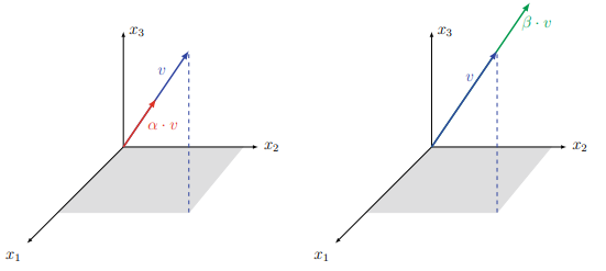
数学代写|线性代数代写linear algebra代考|Vectors and Vector Spaces
In the last section, we saw that the set of $4 \times 4$ images, together with real scalars, satisfies several natural properties. There are in fact many other sets of objects that also have these properties.
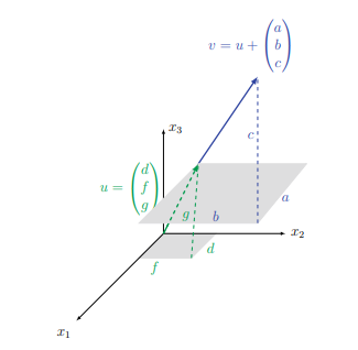
One class of objects with these properties are the vectors that you may have seen in a course in multivariable calculus or physics. In those courses, vectors are objects with a fixed number, say $n$, of values put together into an ordered tuple. That is, the word vector may bring to mind something that looks like $\langle a, b\rangle,\langle a, b, c\rangle$, or $\left\langle a_{1}, a_{2}, \ldots, a_{n}\right\rangle$. Maybe you have even seen notation like any of the following:
$$
(a, b), \quad(a, b, c), \quad\left(a_{1}, a_{2}, \ldots, a_{n}\right),\left(\begin{array}{l}
a \
b \
c
\end{array}\right), \quad\left[\begin{array}{c}
a \
b \
c
\end{array}\right],\left(\begin{array}{c}
a_{1} \
a_{2} \
\vdots \
a_{n}
\end{array}\right),\left[\begin{array}{c}
a_{1} \
a_{2} \
\vdots \
a_{n}
\end{array}\right]
$$
called vectors as well.
In this section, we generalize the notion of a vector. In particular, we will understand that images and other classes of objects can be vectors in an appropriate context. When we consider objects like brain images, radiographs, or heat state signatures, it is often useful to understand them as collections having certain natural mathematical properties. Indeed, we will develop mathematical tools that can be used on all such sets, and these tools will be instrumental in accomplishing our application tasks.
We haven’t yet made the definition of a vector space (or even a vector) rigorous. We still have some more setup to do. In this text, we will primarily use two scalar fields ${ }^{6}: \mathbb{R}$ and $Z_{2}$. The field $Z_{2}$ is the two element (or binary) set ${0,1}$ with addition and multiplication defined modulo 2 . That is, addition defined modulo 2, means that:
$$
0+0=0, \quad 0+1=1+0=1, \quad \text { and } 1+1=0
$$
And, multiplication defined modulo 2 means
$$
0 \cdot 0=0, \quad 0 \cdot 1=1 \cdot 0=0, \quad \text { and } 1 \cdot 1=1 .
$$
We can think of the two elements as “on” and “off” and the operations as binary operations. If we add 1 , we flip the switch and if we add 0 , we do nothing. We know that $Z_{2}$ is closed under scalar multiplication and vector addition.
线性代数代考
数学代写|线性代数代写linear algebra代考|The Geometry of Systems of Equations
事实证明,两个变量方程组的解与方程中线的几何形状之间存在密切联系。R2. 我们回顾一下解决以下系统的图形方法。尽管您可能已经在之前的课程中完成了此操作,但我们将其包含在此处,以便您可以将这些知识放入定理 2.2.20 中分类的方程组的解集的上下文中。
我们从以下简单示例开始:
示例 2.2.27 让我们考虑在=(2 −3),在=(1 1), 和在=(2 3)∈R2. 假设我们想知道我们是否可以表达在使用算术运算在和在. 换句话说,我们想知道是否有标量X,是以便
(2 −3)=X⋅(1 1)+是⋅(2 3).
我们可以重写向量方程的右手边,这样我们就有两个向量的方程
(2 −3)=(X+2是 X+3是).
具有 2 个方程和 2 个变量的线性方程组的等效系统是
X+2是=2 X+3是=−3
方程(2.18)和(2.19)是线方程R2,即对的集合(X,是)满足每个方程的就是每条相应线上的点集。因此,发现X和是满足这两个方程等于找到所有点(X,是)在两条线上。如果我们绘制这两条线,我们可以看到它们似乎在一点交叉,(12,−5), 没有其他地方,所以我们估计X=12和是=−5是两个方程的唯一解。(参见图 2.9。)您还可以通过代数验证(12,5)是系统的解决方案。
数学代写|线性代数代写linear algebra代考|Images and Image Arithmetic
在部分2.1我们看到,如果你添加两个图像,你会得到一个新图像,如果你将一个图像乘以一个标量,你会得到一个新图像。我们将矩形像素化图像表示为值数组,或者等效地表示为灰度补丁的矩形数组。在数码摄影的背景下,这是一个非常自然的想法。
回想 2.1 节中给出的图像定义。我们在这里重复一遍,并通过一些具有不同几何排列的图像示例来遵循定义。
图像是具有相关几何排列的实数值的有限有序列表。
在图 2.11 中可以看到数组的四个示例以及指定补丁顺序的索引系统。作为图像,每个补丁也会有一个数值表示补丁的亮度(图中未显示)。第一种是常用于数码摄影的常规像素阵列。第二个是六边形图案,也可以很好地平铺平面。第三张是按国家划分的非洲大陆和马达加斯加地图。第四个是朝向感兴趣区域中心的具有增强分辨率的方形像素集。从定义中应该清楚图像不是矩阵。只有第一个示例可能与矩阵混淆。
我们首先修复像素的特定几何排列(并让n表示排列中的像素数)。然后通过其(有序)强度值精确描述图像。确定这一点后,我们将上一节中开发的图像上的标量乘法和加法的概念形式化。
数学代写|线性代数代写linear algebra代考|Vectors and Vector Spaces
在上一节中,我们看到了4×4图像与实标量一起满足几个自然属性。事实上,还有许多其他对象集也具有这些属性。
具有这些属性的一类对象是您可能在多变量微积分或物理课程中看到的向量。在这些课程中,向量是具有固定数量的对象,例如n, 的值放在一个有序的元组中。也就是说,词向量可能会让人想起一些看起来像⟨一个,b⟩,⟨一个,b,C⟩, 或者⟨一个1,一个2,…,一个n⟩. 也许您甚至见过以下任何一种符号:
(一个,b),(一个,b,C),(一个1,一个2,…,一个n),(一个 b C),[一个 b C],(一个1 一个2 ⋮ 一个n),[一个1 一个2 ⋮ 一个n]
也称为向量。
在本节中,我们概括了向量的概念。特别是,我们将理解图像和其他类别的对象可以是适当上下文中的向量。当我们考虑诸如大脑图像、射线照片或热状态特征之类的对象时,将它们理解为具有某些自然数学属性的集合通常很有用。事实上,我们将开发可用于所有此类集合的数学工具,这些工具将有助于完成我们的应用任务。
我们还没有严格定义向量空间(甚至向量)。我们还有更多的设置要做。在本文中,我们将主要使用两个标量字段6:R和从2. 场从2是二元(或二元)集0,1加法和乘法定义模 2 。也就是说,加法定义模 2,意味着:
0+0=0,0+1=1+0=1, 和 1+1=0
并且,乘法定义模 2 意味着
0⋅0=0,0⋅1=1⋅0=0, 和 1⋅1=1.
我们可以将这两个元素视为“on”和“off”,并将操作视为二进制操作。如果我们添加 1 ,我们翻转开关,如果我们添加 0 ,我们什么也不做。我们知道从2在标量乘法和向量加法下是闭合的。

统计代写请认准statistics-lab™. statistics-lab™为您的留学生涯保驾护航。
金融工程代写
金融工程是使用数学技术来解决金融问题。金融工程使用计算机科学、统计学、经济学和应用数学领域的工具和知识来解决当前的金融问题,以及设计新的和创新的金融产品。
非参数统计代写
非参数统计指的是一种统计方法,其中不假设数据来自于由少数参数决定的规定模型;这种模型的例子包括正态分布模型和线性回归模型。
广义线性模型代考
广义线性模型(GLM)归属统计学领域,是一种应用灵活的线性回归模型。该模型允许因变量的偏差分布有除了正态分布之外的其它分布。
术语 广义线性模型(GLM)通常是指给定连续和/或分类预测因素的连续响应变量的常规线性回归模型。它包括多元线性回归,以及方差分析和方差分析(仅含固定效应)。
有限元方法代写
有限元方法(FEM)是一种流行的方法,用于数值解决工程和数学建模中出现的微分方程。典型的问题领域包括结构分析、传热、流体流动、质量运输和电磁势等传统领域。
有限元是一种通用的数值方法,用于解决两个或三个空间变量的偏微分方程(即一些边界值问题)。为了解决一个问题,有限元将一个大系统细分为更小、更简单的部分,称为有限元。这是通过在空间维度上的特定空间离散化来实现的,它是通过构建对象的网格来实现的:用于求解的数值域,它有有限数量的点。边界值问题的有限元方法表述最终导致一个代数方程组。该方法在域上对未知函数进行逼近。[1] 然后将模拟这些有限元的简单方程组合成一个更大的方程系统,以模拟整个问题。然后,有限元通过变化微积分使相关的误差函数最小化来逼近一个解决方案。
tatistics-lab作为专业的留学生服务机构,多年来已为美国、英国、加拿大、澳洲等留学热门地的学生提供专业的学术服务,包括但不限于Essay代写,Assignment代写,Dissertation代写,Report代写,小组作业代写,Proposal代写,Paper代写,Presentation代写,计算机作业代写,论文修改和润色,网课代做,exam代考等等。写作范围涵盖高中,本科,研究生等海外留学全阶段,辐射金融,经济学,会计学,审计学,管理学等全球99%专业科目。写作团队既有专业英语母语作者,也有海外名校硕博留学生,每位写作老师都拥有过硬的语言能力,专业的学科背景和学术写作经验。我们承诺100%原创,100%专业,100%准时,100%满意。
随机分析代写
随机微积分是数学的一个分支,对随机过程进行操作。它允许为随机过程的积分定义一个关于随机过程的一致的积分理论。这个领域是由日本数学家伊藤清在第二次世界大战期间创建并开始的。
时间序列分析代写
随机过程,是依赖于参数的一组随机变量的全体,参数通常是时间。 随机变量是随机现象的数量表现,其时间序列是一组按照时间发生先后顺序进行排列的数据点序列。通常一组时间序列的时间间隔为一恒定值(如1秒,5分钟,12小时,7天,1年),因此时间序列可以作为离散时间数据进行分析处理。研究时间序列数据的意义在于现实中,往往需要研究某个事物其随时间发展变化的规律。这就需要通过研究该事物过去发展的历史记录,以得到其自身发展的规律。
回归分析代写
多元回归分析渐进(Multiple Regression Analysis Asymptotics)属于计量经济学领域,主要是一种数学上的统计分析方法,可以分析复杂情况下各影响因素的数学关系,在自然科学、社会和经济学等多个领域内应用广泛。
MATLAB代写
MATLAB 是一种用于技术计算的高性能语言。它将计算、可视化和编程集成在一个易于使用的环境中,其中问题和解决方案以熟悉的数学符号表示。典型用途包括:数学和计算算法开发建模、仿真和原型制作数据分析、探索和可视化科学和工程图形应用程序开发,包括图形用户界面构建MATLAB 是一个交互式系统,其基本数据元素是一个不需要维度的数组。这使您可以解决许多技术计算问题,尤其是那些具有矩阵和向量公式的问题,而只需用 C 或 Fortran 等标量非交互式语言编写程序所需的时间的一小部分。MATLAB 名称代表矩阵实验室。MATLAB 最初的编写目的是提供对由 LINPACK 和 EISPACK 项目开发的矩阵软件的轻松访问,这两个项目共同代表了矩阵计算软件的最新技术。MATLAB 经过多年的发展,得到了许多用户的投入。在大学环境中,它是数学、工程和科学入门和高级课程的标准教学工具。在工业领域,MATLAB 是高效研究、开发和分析的首选工具。MATLAB 具有一系列称为工具箱的特定于应用程序的解决方案。对于大多数 MATLAB 用户来说非常重要,工具箱允许您学习和应用专业技术。工具箱是 MATLAB 函数(M 文件)的综合集合,可扩展 MATLAB 环境以解决特定类别的问题。可用工具箱的领域包括信号处理、控制系统、神经网络、模糊逻辑、小波、仿真等。