如果你也在 怎样代写计算复杂度理论Computational complexity theory这个学科遇到相关的难题,请随时右上角联系我们的24/7代写客服。
计算复杂度理论的重点是根据资源使用情况对计算问题进行分类,并将这些类别相互联系起来。计算问题是一项由计算机解决的任务。一个计算问题是可以通过机械地应用数学步骤来解决的,比如一个算法。
statistics-lab™ 为您的留学生涯保驾护航 在代写计算复杂度理论Computational complexity theory方面已经树立了自己的口碑, 保证靠谱, 高质且原创的统计Statistics代写服务。我们的专家在代写计算复杂度理论Computational complexity theory代写方面经验极为丰富,各种代写计算复杂度理论Computational complexity theory相关的作业也就用不着说。
我们提供的计算复杂度理论Computational complexity theory及其相关学科的代写,服务范围广, 其中包括但不限于:
- Statistical Inference 统计推断
- Statistical Computing 统计计算
- Advanced Probability Theory 高等概率论
- Advanced Mathematical Statistics 高等数理统计学
- (Generalized) Linear Models 广义线性模型
- Statistical Machine Learning 统计机器学习
- Longitudinal Data Analysis 纵向数据分析
- Foundations of Data Science 数据科学基础
数学代写|计算复杂度理论代写Computational complexity theory代考|Curie-Weiss Model
An important aspect of the Ising model is given by its dimension $D$. Notably, for $D=1$, the Ising model has no phase transitions at finite temperature. For $D=2$, according to the Onsager’s solution, there is a phase transition (at a finite temperature). Then, in higher dimensions, although a phase transition can be observed, the definition of an analytical solution still constitutes an open problem. In particular, for $D=3$, the problem has been solved only by a numerical approach,
while for $D>3$ a solution is still required. Here, we briefly present a toy model that allows to describe the behavior of ferromagnetic transitions at infinite dimension, i.e., the Curie-Weiss (CW hereinafter) model. Remarkably the latter, despite being a toy model, has been proven to have a great relevance both in statistical mechanics and in information theory. The infinite dimension of the system entails that, in the CW model, each spin is connected with all the others. Accordingly, its Hamiltonian reads
$$
H\left(\sigma_{1}, \ldots \sigma_{n}\right)=-\frac{1}{N} \sum_{(i<j)} \sigma_{i} \sigma_{j}-h \sum_{i=1}^{N} \sigma_{i}
$$
As result, using the jargon of graph theory, the CW model defines a complete graph of $N$ nodes and $N(N-1) / 2$ links. Then, using the magnetization $m$ before introduced, and without considering the contribution of external fields, the Hamiltonian of this model takes following form
$$
H\left(\sigma_{1}, \ldots \sigma_{n}\right)=-\frac{N}{2} m^{2}+O(1)
$$
As above reported, for computing the expected values of physical quantities of systems like those we are considering, we need to compute the partition function of the system that in this case is equal to
$$
Z=\sum_{\left{\sigma_{i}\right}} e^{-\beta H\left(\sigma_{1}, \ldots, \sigma_{N}\right)}
$$
with $H$ defined in Eq. (2.11). Now, further calculations are required for solving the equation, as for instance, for computing the summation over the spin variables appearing in Eq. (2.13). However, without to show the whole mathematical derivation, we only report the final equation of state of the CW model
$$
m=\tanh (\beta J m+\beta h)
$$
数学代写|计算复杂度理论代写Computational complexity theory代考|Landau Theory of Phase Transitions
The approaches here presented for studying the phenomenology of phase transitions by analytical methods allow to compute the partition function of a system. Therefore, at least in principle, a number of quantities can be computed according to Eq. (2.6). For a reason that will be soon explained, it is now worth to introduce an important thermodynamic potential, named “free energy,” that allows to study the state of equilibrium of a system. In particular, the so-called Helmholtz free energy is defined as $F=U-T S$, with $U$ internal energy, $T$ temperature, and $S$ entropy. So, since the second law of thermodynamics states that a system evolves toward
the state that maximizes its entropy, this law can be re-paraphrased stating that the state of equilibrium of a system corresponds to one that minimizes its free energy $F$. Now, we can motivate why we moved from the brief remark on the role of the partition function to the introduction of the free energy. Notably, a very important relation links the two quantities
$$
-k_{b} T \ln Z=U-T S
$$
As a result, we have $Z=e^{-\beta F}$. Here, the mean-field theory allows to obtain an approximated phase diagram of the system. However, when the latter is close to the critical point (e.g., the critical temperature), its behavior can be analyzed by using the formulation introduced by Landau, named “Landau theory of phase transitions.” The underlying assumption of this theory is that a system close to the critical point has a small order parameter (i.e., $m$ ), which leads to the expression of the free energy as the following summation of power series:
$$
F(T ; m)=f(T ; 0)+\frac{1}{2} a(T) m^{2}+\frac{1}{4 !} b(T) m^{4}+\ldots
$$
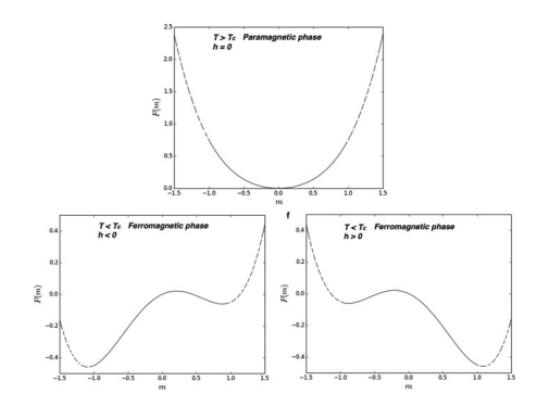
with $a(T)$ and $b(T)$ coefficients that can be computed analytically. For instance, Fig. $2.2$ shows the free energy of the CW model (with $h=0$ ). In particular, for $T>T_{c}$ there is only one minimum of free energy ( $\left.m=0\right)$, corresponding to the state defined “paramagnetic phase.” Instead, for $T<T_{c}$ there are two possible minima of free energy, and the symmetry $m \rightarrow-m$ is spontaneously broken (phenomenon known as “symmetry breaking”).
数学代写|计算复杂度理论代写Computational complexity theory代考|Numerical Simulations
After introducing the Ising model, and some methods of approximation for studying special cases (e.g., $D \geq 4$ ), we can move toward a quick presentation of computational methods for performing the related numerical simulations. This part is of particular interest for achieving a preliminary idea on how to implement numerical simulations using networked agents, i.e., agents arranged in graphs, no matter if regular (as in the case of the Ising model) or random (as in the case of Complex Networks below discussed). In general, if we want to investigate the properties of a system using, for example, the formalism of the canonical ensemble, we have to deal with a system described by the macrostate $(N, V, T)$ (i.e., number of particles, volume, and temperature). Given a microstate $\sigma$, a generic observable can be indicated as $O(\sigma)$, and its average value at equilibrium is
$$
\langle O(\sigma)\rangle=\frac{1}{Z} \sum_{\sigma} e^{-\beta H(\sigma)}
$$
thus, without the knowledge of the partition function $Z$, we cannot compute the average value of our observable $O(\sigma)$. A further example, previously mentioned, is given by the Ising model, where numerical simulations become mandatory for studying its behavior for $D \geq 3$. So, in order to overcome this limit, we can adopt Monte Carlo (MC hereinafter) methods for computing the value of the quantities we are interested in. The underlying idea of MC methods is to generate subset configurations (from the whole phase space), with a weight given by the Boltzmann statistics, that are representative for the entire ensemble. So, generating, for example, $M$ configurations, we can have an estimate of the observable computing its average value, i.e.,
$$
\langle O(\sigma)\rangle=\frac{1}{M} \sum_{i=1}^{M} O_{i}(\sigma)
$$
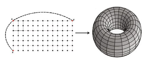
Therefore, we are able to compute the average value of a physical quantity avoiding to deal with the partition function $Z$ of the system (as in Eq. (2.17)). Now, before to proceed, it is worth to remind that the analytical solutions of a system (e.g., the Ising model) usually are computed considering the thermodynamic limit (i.e., $N \rightarrow \infty$ ). So, from a computational point of view, the first problem is how to approximate such limit/condition. In the case of the Ising model, a viable solution is given by the implementation of lattices which size is sufficiently big, removing the finite
size effect using a simple trick, i.e., generating lattices with continuous boundary conditions. Actually, under this condition, a bidimensional lattice takes the form of a toroid. In particular, this transformation can be easily performed by connecting the sites at the edges of the lattice. For instance, Fig. $2.3$ shows an example focusing on the site named $x$, that is, connected to the sites $y$ and $z$, increasing its amount of bonds up to four. Going back to the problem of performing a numerical simulation of the Ising model, we can implement different algorithms. Here, we refer to one of the most famous, i.e., the Metropolis algorithm. We remind that our aim is measuring the value of parameters like the magnetization at equilibrium. As we know from theory, at low temperatures we expect a ferromagnetic phase, i.e., a system close to the order, while at high temperatures a paramagnetic phase, i.e., a disordered system. The Metropolis algorithm is very simple, and its steps are:
- Randomly select a site $i$ and compute the local $\Delta E$ associated to its spin flip
- IF $(\Delta E \leq 0)$ : accept the flip;
ELSE: accept the flip with probability $e^{\frac{-\Delta E}{k_{b} T}}$
repeated until an equilibrium state is reached. The $\Delta E$ indicates a local difference in energy, i.e., computed considering only the selected site and its nearest neighbors.
计算复杂度理论代考
数学代写|计算复杂度理论代写Computational complexity theory代考|Curie-Weiss Model
Ising 模型的一个重要方面是它的维度D. 值得注意的是,对于D=1,Ising 模型在有限温度下没有相变。为了D=2,根据 Onsager 的解,存在相变(在有限温度下)。然后,在更高维度上,虽然可以观察到相变,但解析解的定义仍然是一个悬而未决的问题。特别是,对于D=3, 该问题仅通过数值方法解决,
而对于D>3仍然需要一个解决方案。在这里,我们简要介绍了一个玩具模型,该模型可以描述无限维度下铁磁跃迁的行为,即居里-魏斯(以下简称 CW)模型。值得注意的是,尽管后者是一个玩具模型,但已被证明在统计力学和信息论中都具有很大的相关性。系统的无限维度意味着,在 CW 模型中,每个自旋都与所有其他自旋相连。因此,它的哈密顿量为
H(σ1,…σn)=−1ñ∑(一世<j)σ一世σj−H∑一世=1ñσ一世
结果,使用图论的术语,CW模型定义了一个完整的图ñ节点和ñ(ñ−1)/2链接。然后,使用磁化米在介绍之前,在不考虑外场贡献的情况下,该模型的哈密顿量具有以下形式
H(σ1,…σn)=−ñ2米2+○(1)
如上所述,为了计算我们正在考虑的系统的物理量的期望值,我们需要计算系统的配分函数,在这种情况下等于
Z=\sum_{\left{\sigma_{i}\right}} e^{-\beta H\left(\sigma_{1}, \ldots, \sigma_{N}\right)}Z=\sum_{\left{\sigma_{i}\right}} e^{-\beta H\left(\sigma_{1}, \ldots, \sigma_{N}\right)}
和H在方程式中定义。(2.11)。现在,需要进一步计算来求解方程,例如,计算方程中出现的自旋变量的总和。(2.13)。然而,在没有展示整个数学推导的情况下,我们只报告了 CW 模型的最终状态方程
米=腥(bĴ米+bH)
数学代写|计算复杂度理论代写Computational complexity theory代考|Landau Theory of Phase Transitions
这里提出的通过分析方法研究相变现象学的方法允许计算系统的配分函数。因此,至少在原则上,可以根据方程式计算出许多量。(2.6)。出于即将解释的原因,现在值得引入一个重要的热力学势,称为“自由能”,它允许研究系统的平衡状态。特别是,所谓的亥姆霍兹自由能定义为F=在−吨小号, 和在内能,吨温度,和小号熵。因此,由于热力学第二定律指出,系统向
熵最大化的状态,该定律可以重新解释为系统的平衡状态对应于其自由能最小化的状态F. 现在,我们可以解释为什么我们从对配分函数的作用的简短评论转移到引入自由能。值得注意的是,一个非常重要的关系将这两个量联系起来
−ķb吨ln从=在−吨小号
结果,我们有从=和−bF. 在这里,平均场理论允许获得系统的近似相图。然而,当后者接近临界点(例如,临界温度)时,可以使用朗道引入的公式来分析其行为,称为“朗道相变理论”。该理论的基本假设是接近临界点的系统具有较小的阶参数(即,米),这导致自由能表示为以下幂级数的总和:
F(吨;米)=F(吨;0)+12一个(吨)米2+14!b(吨)米4+…
和一个(吨)和b(吨)可以分析计算的系数。例如,图。2.2显示了 CW 模型的自由能(与H=0)。特别是,对于吨>吨C只有一个最小自由能(米=0),对应于状态定义的“顺磁相”。相反,对于吨<吨C自由能有两个可能的最小值,对称性米→−米被自发破坏(称为“对称破坏”的现象)。
数学代写|计算复杂度理论代写Computational complexity theory代考|Numerical Simulations
在介绍了 Ising 模型,以及一些用于研究特殊情况的逼近方法(例如,D≥4),我们可以快速介绍用于执行相关数值模拟的计算方法。这部分对于初步了解如何使用网络代理(即以图形排列的代理,无论是规则的(如 Ising 模型的情况)还是随机的(如下面讨论的复杂网络)。一般来说,如果我们想使用例如规范集成的形式来研究系统的属性,我们必须处理由宏观状态描述的系统(ñ,在,吨)(即,粒子数、体积和温度)。给定一个微观状态σ, 一个通用的 observable 可以表示为○(σ),其均衡时的平均值为
⟨○(σ)⟩=1从∑σ和−bH(σ)
因此,在不知道配分函数的情况下从,我们无法计算可观察的平均值○(σ). 前面提到的另一个例子是 Ising 模型,其中数值模拟成为研究其行为的必要条件D≥3. 因此,为了克服这个限制,我们可以采用蒙特卡罗(以下简称 MC)方法来计算我们感兴趣的量的值。MC 方法的基本思想是生成子集配置(从整个相空间),具有由玻尔兹曼统计给出的权重,代表整个集合。因此,例如,生成米配置,我们可以估计可观察的计算其平均值,即
⟨○(σ)⟩=1米∑一世=1米○一世(σ)
因此,我们能够计算物理量的平均值,从而避免处理配分函数从系统的(如方程(2.17))。现在,在继续之前,值得提醒的是,系统的解析解(例如,伊辛模型)通常是在考虑热力学极限(即,ñ→∞)。因此,从计算的角度来看,第一个问题是如何近似这种限制/条件。在伊辛模型的情况下,一个可行的解决方案是通过实现足够大的格子来给出一个可行的解决方案,消除有限的
尺寸效应使用一个简单的技巧,即生成具有连续边界条件的晶格。实际上,在这种情况下,二维晶格呈环形。特别是,通过连接晶格边缘的位点可以很容易地进行这种转换。例如,图。2.3显示了一个专注于名为的站点的示例X,即连接到站点是和和,将其债券数量增加到四个。回到对 Ising 模型进行数值模拟的问题,我们可以实现不同的算法。在这里,我们指的是最著名的算法之一,即 Metropolis 算法。我们提醒我们,我们的目标是测量平衡磁化强度等参数的值。从理论上我们知道,在低温下,我们期望一个铁磁相,即接近有序的系统,而在高温下,我们期望一个顺磁相,即无序系统。Metropolis 算法非常简单,其步骤为:
- 随机选择一个站点一世并计算本地Δ和与其旋转翻转相关联
- 如果(Δ和≤0):接受翻转;
ELSE:接受概率翻转和−Δ和ķb吨
重复直到达到平衡状态。这Δ和表示能量的局部差异,即仅考虑所选站点及其最近的邻居来计算。

统计代写请认准statistics-lab™. statistics-lab™为您的留学生涯保驾护航。
金融工程代写
金融工程是使用数学技术来解决金融问题。金融工程使用计算机科学、统计学、经济学和应用数学领域的工具和知识来解决当前的金融问题,以及设计新的和创新的金融产品。
非参数统计代写
非参数统计指的是一种统计方法,其中不假设数据来自于由少数参数决定的规定模型;这种模型的例子包括正态分布模型和线性回归模型。
广义线性模型代考
广义线性模型(GLM)归属统计学领域,是一种应用灵活的线性回归模型。该模型允许因变量的偏差分布有除了正态分布之外的其它分布。
术语 广义线性模型(GLM)通常是指给定连续和/或分类预测因素的连续响应变量的常规线性回归模型。它包括多元线性回归,以及方差分析和方差分析(仅含固定效应)。
有限元方法代写
有限元方法(FEM)是一种流行的方法,用于数值解决工程和数学建模中出现的微分方程。典型的问题领域包括结构分析、传热、流体流动、质量运输和电磁势等传统领域。
有限元是一种通用的数值方法,用于解决两个或三个空间变量的偏微分方程(即一些边界值问题)。为了解决一个问题,有限元将一个大系统细分为更小、更简单的部分,称为有限元。这是通过在空间维度上的特定空间离散化来实现的,它是通过构建对象的网格来实现的:用于求解的数值域,它有有限数量的点。边界值问题的有限元方法表述最终导致一个代数方程组。该方法在域上对未知函数进行逼近。[1] 然后将模拟这些有限元的简单方程组合成一个更大的方程系统,以模拟整个问题。然后,有限元通过变化微积分使相关的误差函数最小化来逼近一个解决方案。
tatistics-lab作为专业的留学生服务机构,多年来已为美国、英国、加拿大、澳洲等留学热门地的学生提供专业的学术服务,包括但不限于Essay代写,Assignment代写,Dissertation代写,Report代写,小组作业代写,Proposal代写,Paper代写,Presentation代写,计算机作业代写,论文修改和润色,网课代做,exam代考等等。写作范围涵盖高中,本科,研究生等海外留学全阶段,辐射金融,经济学,会计学,审计学,管理学等全球99%专业科目。写作团队既有专业英语母语作者,也有海外名校硕博留学生,每位写作老师都拥有过硬的语言能力,专业的学科背景和学术写作经验。我们承诺100%原创,100%专业,100%准时,100%满意。
随机分析代写
随机微积分是数学的一个分支,对随机过程进行操作。它允许为随机过程的积分定义一个关于随机过程的一致的积分理论。这个领域是由日本数学家伊藤清在第二次世界大战期间创建并开始的。
时间序列分析代写
随机过程,是依赖于参数的一组随机变量的全体,参数通常是时间。 随机变量是随机现象的数量表现,其时间序列是一组按照时间发生先后顺序进行排列的数据点序列。通常一组时间序列的时间间隔为一恒定值(如1秒,5分钟,12小时,7天,1年),因此时间序列可以作为离散时间数据进行分析处理。研究时间序列数据的意义在于现实中,往往需要研究某个事物其随时间发展变化的规律。这就需要通过研究该事物过去发展的历史记录,以得到其自身发展的规律。
回归分析代写
多元回归分析渐进(Multiple Regression Analysis Asymptotics)属于计量经济学领域,主要是一种数学上的统计分析方法,可以分析复杂情况下各影响因素的数学关系,在自然科学、社会和经济学等多个领域内应用广泛。
MATLAB代写
MATLAB 是一种用于技术计算的高性能语言。它将计算、可视化和编程集成在一个易于使用的环境中,其中问题和解决方案以熟悉的数学符号表示。典型用途包括:数学和计算算法开发建模、仿真和原型制作数据分析、探索和可视化科学和工程图形应用程序开发,包括图形用户界面构建MATLAB 是一个交互式系统,其基本数据元素是一个不需要维度的数组。这使您可以解决许多技术计算问题,尤其是那些具有矩阵和向量公式的问题,而只需用 C 或 Fortran 等标量非交互式语言编写程序所需的时间的一小部分。MATLAB 名称代表矩阵实验室。MATLAB 最初的编写目的是提供对由 LINPACK 和 EISPACK 项目开发的矩阵软件的轻松访问,这两个项目共同代表了矩阵计算软件的最新技术。MATLAB 经过多年的发展,得到了许多用户的投入。在大学环境中,它是数学、工程和科学入门和高级课程的标准教学工具。在工业领域,MATLAB 是高效研究、开发和分析的首选工具。MATLAB 具有一系列称为工具箱的特定于应用程序的解决方案。对于大多数 MATLAB 用户来说非常重要,工具箱允许您学习和应用专业技术。工具箱是 MATLAB 函数(M 文件)的综合集合,可扩展 MATLAB 环境以解决特定类别的问题。可用工具箱的领域包括信号处理、控制系统、神经网络、模糊逻辑、小波、仿真等。